Comparative Analysis of MCDA Techniques for Identifying Erosion-Prone Areas in the Burhanpur Watershed in Central India for the Purposes of Sustainable Watershed Management

Abstract

The degradation of land and increasing water scarcity are existing challenges for agricultural sustainability, necessitating the implementation of improved soil-conservation practices at the watershed scale. The identification and selection of critical/prone areas based on erosion-governing criteria is essential and helps in the execution of the management process for determining priority. This study prioritizes erosion-prone sub-watersheds (alternatives) based on morphometric parameters (multiple criteria) via five Multi-Criteria Decision Analysis (MCDA) approaches, i.e., AHP: Analytical Hierarchy Process; TOPSIS: Technique for Order of Preference by Similarity to Ideal Solution; VIKOR: VIseKriterijumska Optimizacija I Kompromisno Resenje; SAW: Simple Additive Weighting; and CF: Compound Factor. Based on their priority score, 19 sub-watersheds were classified into four priority classes: low priority (0–0.25), moderate priority (0.25–0.50), high priority (0.50–0.75), and very high priority (0.75–1). The results revealed that about 8.34–30.15% area of the Burhanpur watershed is critically prone to erosion, followed by 23.38–52.05% area classed as high priority, 7.47–49.99% area classed as moderate priority, and 10.33–18.28% area classed as low priority. Additionally, four indices—percentage of changes (∆P), intensity of changes (∆I), the Spearman rank correlation coefficient test (SCCT), and the Kendall tau correlation coefficient test (KTCCT)—were employed to compare the models. This study confirms the efficacy of morphometric parameters for prioritizing sub-watersheds to preserve soil and the environment, particularly in areas for which limited information is available.

1. Introduction

Land and water are not only valuable natural resources, but also critical for sustaining life and agricultural production. The ongoing degradation of land, coupled with increasing water scarcity, is a major concern for achieving sustainability in agriculture [1,2]. Globally, it has been reported that approximately 15% of ice-free land surface is under degradation, and in India, this figure is as high as 45% of the country’s geographical area [3,4]. Additionally, India is losing its valuable soil at a rate of approximately 16.4 tons/ha per year due to erosion, deforestation, and other destructive agents [5]. Soil erosion is a serious environmental hazard that contributes to land degradation [6,7]. Given that soil formation is a slow process that can take up to 300 years to produce a 1 cm layer of soil [8], it is necessary to conserve soil resources through better management practices in erosion-prone areas, with a focus on watershed-scale management measures [9] to mitigate soil erosion and conserve land and soil resources.

Watersheds are natural drainage units that respond to rainfall, depending on factors such as climate, land use, hydrogeology, and morphology, to generate runoff [10]. As such, watersheds represent an ideal unit for both land and water resources management. Watershed-level management strategies have a positive impact on resource productivity [11,12,13]. The drainage morphometry and parameters of watersheds are responsible for runoff, and thereby erosion phenomena and their characteristics occurring within watersheds [14,15,16]. Morphometric parameters are quantitative representations of watershed geometry and topography [17,18], and they help in understanding a watershed’s linear drainage system, its areal pattern, and its relief behavior for the purposes of hydrological engineering [19,20]. These parameters, which include linear, areal, and relief aspects of the watershed, are derived during morphometric analysis of watershed topography [21,22,23,24]. Several studies have demonstrated the potential of Remote Sensing (RS) and Geographical Information Systems (GIS) for conducting morphometric analysis [25,26,27,28,29] and providing valuable information for watershed management and planning. Moreover, remote sensing-based Digital Elevation Models (DEMs) have been widely used for topography-based studies [30,31,32].

Understanding watershed morphometry assists watershed management, in an efficient and integrated manner, to increase productivity with optimum use of resources. Moreover, it helps in planning degradation neutrality strategies through sub-watersheds prioritization [12,33]. Recently, researchers have successfully implemented morphometric parameters as criteria in the prioritization of sub-watersheds by applying Multi Criteria Decision Analysis (MCDA) techniques [19,34,35,36,37]. MCDA techniques were used for complex decision making while considering a set of criteria to improve decision accuracy [8,38,39,40,41]. Several MCDA techniques, such as Analytical Hierarchy Process (AHP) [42], Technique for Order of Preference by Similarity to Ideal Solution (TOPSIS) [43], VIseKriterijumska Optimizacija I Kompromisno Resenje (VIKOR) [44], Simple Additive Weighting (SAW), compound factor (CF) analysis, etc., have been successfully used by several researchers for accurate decision making [5,10,19,34,35,45,46,47,48,49,50]. Hembram and Saha [45] prioritized sub-watersheds of the Chota Nagpur Plateau in Jharkhand using fuzzy AHP and the compound factor (CF) approach. The results obtained from both analyses highlight sub-watersheds 6 and 13 as very highly erosion-prone areas. The study demonstrated the effectiveness of morphometric indices in assessing erodibility priority at the sub-basin scale. The authors of [51] applied the analytical network process and fuzzy logic theory when considering the interrelationship of environmental and geomorphic factors in the watershed of the Araz River basin of Iran. A criteria-based decision framework was developed for the calculation of the watershed health scores (WHS) and to prioritize watersheds. The study recommended the potential of such frameworks for the identification of highly critical zones, especially in data-scarce areas.

A number of studies have been undertaken in recent years to map erosion-prone areas using individual MCDA on GIS- and DEM-derived morphometric data. However, there have been few studies that apply multiple MCDA techniques simultaneously and compare them to determine the optimal model. Thus, in the present study, a number of MCDA approaches (AHP, TOPSIS, VIKOR, SAW, and CF) were applied to prioritize erosion-prone sites in the Burhanpur watershed, and their performance was evaluated. Using GIS and RS techniques, this study analyzes fourteen morphometric parameters to effectively prioritize the nineteen sub-watersheds, providing valuable information for the development of improved decision support and a comprehensive land degradation management plan in the Burhanpur watershed in Central India.

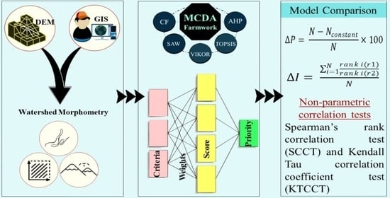
2. Materials and Methods

2.1. Study Area and Data

The Burhanpur is situated in the Upper Tapi river basin in Central India. The geographic boundaries of the watershed encompass a longitude range of 75°55′ E to 78°18′14″ E and a latitude range of 21°1′51″ N to 22°1′52″ N (Figure 1). Within this area, the watershed spans approximately 10,585 km². The elevation in the region ranges from 188 to 1171 m above mean sea level, while the average annual rainfall is around 900 mm. The study area primarily consists of clayey to loamy clayey soils [52], with land use types including agriculture, range lands, water bodies, barren land, built-up areas, and forests. The geomorphometric parameters of the Burhanpur watershed were quantified using Remote Sensing (RS) data and Geographic Information System (GIS) techniques. The Shuttle Radar Topography Mission (SRTM) 1 arc-second Digital Elevation Model (DEM) from the USGS Earth Resources Observation and Science (EROS) Center archive was utilized to obtain elevation and topographic information for the study area (source: https://www.usgs.gov/ accessed on 25 August 2023).

Figure 1. Study area with DEM map and river reaches.

2.2. Sub-Watershed Mapping and Morphometric Analysis

For the delineation of the sub-watersheds, SRTM DEM data were obtained and imported into the GIS environment. A delineation procedure involving steps such as ‘fill sinks”, "flow direction”, “flow accumulation”, etc., was performed and the nineteen sub-watersheds were delineated. Further morphometric parameters, related to linear, areal, and relief aspects (mean bifurcation ratio (R_bfm), drainage density (D_d), stream frequency (S_fµ), form factor (F_f), shape factor (F_s), circulatory ratio (R_c), elongation ratio (R_e), constant of channel maintenance (C), infiltration number (I_f), length of overland flow (L_g), texture ratio (T), basin relief (H), relief ratio (R_r), and slope (S)) were computed as per the methods outlined in Table 1 [53,54,55,56]. These sub-watersheds and parameters were subsequently employed as alternatives and criteria, respectively, for prioritizing the sub-watersheds.

Table 1. Computation and relation of morphometric parameters with erosion sensitivity.

Parameters	Quantification	Relation with Erosion Sensitivity	References
Mean bifurcation ratio (Rbfm)	Mean of Rb	DP	[57]
Drainage density (Dd)	Dd = ΣLu/A	DP	[58]
Stream frequency (Sfµ)	Fs = ΣNu/A	DP	[58]
Form factor (Ff)	Ff = A/Lb2	IP	[58,59]
Shape factor (Fs)	Fs = Lb2/A	IP	[59]
Circulatory ratio (Rc)	Rc = 4πA/P2	IP	[18,60]
Elongation ratio (Re)	Re = 1.128√A/Lb	IP	[57]
Constant of channel maintenance (C)	C = 1/Dd	DP	[57]
Infiltration number (If)	If = D × Fs	IP	[61]
Length of overland flow (Lg)	Lg = 1/2Dd	DP	[58]
Texture ratio (T)	T = ΣNu/P	DP	[62]
Basin relief (H)	H = Hmax − Hmin	DP	[63]
Relief ratio (Rr)	Rr = H/L	DP	[57]
Slope (S)	Mean of slope	DP	[23]

Note: DP: directly proportional (higher the parameter value, higher the erosion sensitivity), IP: inversely proportional (higher the parameter value, lower the erosion sensitivity).

2.3. MCDA-Based Sub-Watersheds Prioritization

The morphometric parameters of watersheds play a crucial role in describing various surface phenomena, such as soil erosion, which depend on the hydrology, climate, geology, and geomorphology of the watershed [15]. The erosion sensitivity of the watershed is directly or inversely proportional to these morphometric parameters, which means that higher parameter values correspond to either higher or lower erosion sensitivity. The MCDA techniques involve considering a set of criteria with their relative weights to prioritize alternatives [64,65]. In this study, 14 morphometric parameters (listed in Table 1) were used as criteria to evaluate and prioritize the 19 sub-watersheds using five different MCDA techniques (AHP, TOPSIS, VIKOR, SAW, and CF). These techniques utilize criteria weights and normalized values for the morphometric parameters to calculate the rankings of the sub-watersheds. The flowchart in Figure 2 summarizes the overall methodology employed in this study. The following sections provide a brief overview of the MCDA techniques used.

Figure 2. Depiction of overall methodology employed in this study.

2.3.1. Criteria Weightage for MCDA

The weightage for the different criteria was determined using pairwise comparisons, following the method proposed by Thomas L. Saaty [66]. In this approach, a parameter with a higher impact on erosion sensitivity was given greater preference in the comparison matrix. As mentioned earlier, the pairwise comparisons matrix was constructed using the 14 morphometric parameters as criteria. Subsequently, the weight matrix ${\left[W\right]}_{Q\times 1}$ was calculated, representing the weight of the j-th criterion as w_j (an element of the weight matrix). It is important to note that consistency in pairwise comparisons is essential to derive meaningful weights [67]. Therefore, a consistency check procedure, as described in [68], was followed to ensure consistency. Typically, a consistency ratio below 0.1 indicates consistency in the comparisons, and the weights are considered acceptable [67].

2.3.2. Analytical Hierarchy Process Technique

The AHP technique introduced by T.L. Saaty [42] is one of the most popular and easiest MCDA methods [41]. AHP breaks down the complex problem into hierarchically structured sub-problems to find a solution from among alternatives [42,69]. It involves generation of a decision matrix based on alternatives and criteria followed by normalization of the decision matrix. A further weighted normalized decision matrix is generated [70,71], and priority scores are calculated [72]. The higher the value of the score the higher the priority in the case of AHP. The general steps involved in the AHP process are presented in Appendix A.1.

2.3.3. Technique for Order of Preference by Similarity to Ideal Solution (TOPSIS)

Ching-Lai Hwang and Kwangsun Yoon introduced TOPSIS, which is based on the distance of alternatives from the negative ideal option (NIO) and the positive ideal option (PIO) [43]. It picks the best alternative, which is the one that is found to be nearest to the IPO and farthest from the INO, based on a closeness coefficient [73]. In TOPSIS, a decision matrix based on alternatives and criteria is formulated. This decision matrix is normalized to generate a weighted normalized decision matrix [70,71]. Then, the PIO and the NIO are calculated [34]. Finally, the direct distance and the closeness index are measured to calculate the priority scores [72]. TOPSIS has been widely adopted for prioritization and decision making [46,47,48,50,74]. The general steps involved in the TOPSIS process are presented in Appendix A.2.

2.3.4. VIseKriterijumska Optimizacija I Kompromisno Resenje Technique (VIKOR)

The VIKOR method is a reference-based, well-known MCDA technique introduced by Opricovic and Tzeng which emphasizes the ordering of alternatives based on conflicting parameters (utility vs. regret) [44]. This technique ranks the options on the basis of “distance to optimal solution” [70]. Then, from a normalized weighted matrix, the best and worst values are calculated to generate a boundary-values utility index ($S_i$) and regret index ($R_i$). Finally, these indices are used to generate the final measure ($Q_i$) [75]. The general steps involved in the VIKOR process are presented in Appendix A.3.

2.3.5. Simple Additive Weighting (SAW)

In the SAW technique, each alternative is scored by multiplying the alternative value by criterion weight for all criteria and then summing them to rate the alternative accordingly [34]. The SAW prioritization technique involves generation of a decision matrix based on alternatives and criteria followed by normalization of the decision matrix. A further weighted normalized decision matrix is generated [70,71], and priority scores for alternatives are calculated [72]. The general steps involved in the SAW process are presented in Appendix A.4.

2.3.6. Compound Factor (CF) Technique

The compound factor, also referred to as the combination factor, is a scientifically driven MCDA technique that utilizes scientific knowledge and data [76]. This technique quantitatively estimates the qualitative relationship between parameters (criteria) and the goal of the problem (prioritizing erosion-prone areas in this study), based on scientific knowledge. In this study, equal importance was assigned to all criteria [77]. Thus, the mean of the rating values was calculated as the compound factor, representing the integrated impact of all the parameters. The relationship between different morphometric parameters and erosion sensitivity (sub-watershed prioritization) is provided in Table 1. The general steps involved in the compound factor process are presented in Appendix A.5 [78,79].

2.4. Model Synthesis and Final Priority Ranking

The initial priority scores obtained from different MCDA methods exhibited variation. To ensure comparability, these scores were transformed into final priority values on a uniform scale ranging from 0 to 1 using Equations (1) and (2). Subsequently, the entire range of values was divided into four classes: low priority (0–0.25), moderate priority (0.25–0.50), high priority (0.50–0.75), and very high priority (0.75–1) [34]. Consequently, all 19 sub-watersheds were categorized into these four priority classes.

$$1-\frac{{PV}_{max}-{PV}_i}{{PV}_{max}-{PV}_{min}} for AHP,TOPSIS,SAW$$

(1)

$$\frac{{PV}_{max}-{PV}_i}{{PV}_{max}-{PV}_{min}} for VIKOR,CF$$

(2)

2.5. MCDA Model Comparison

This study employed two change indices, namely the percentage of changes (∆P, see Equation (3)) and the intensity of changes (∆I, see Equation (4)), and two non-parametric statistical tests, namely the Spearman rank correlation coefficient test (SCCT) and the Kendall tau correlation coefficient test (KTCCT), to assess and compare the outcomes of the models in a comparative manner [34,80,81].

$$∆P=\frac{N-N_{constant}}{N}\times 100$$

(3)

$$∆I=\frac{{\sum }_{i=1}^N\frac{rank i\left(r1\right)}{rank i\left(r2\right)}}{N}$$

(4)

The equations involved parameters such as N—representing the total number of alternatives; N_constant—representing the number of alternatives with the same rank; i(r1)—denoting the rank of an alternative in the first method; and i(r2)—representing the rank of the same alternative in the second method.

Non-parametric statistical tests determine the measure of association between ranks obtained by different MCDA techniques [82]. In the SCCT test, Equation (5) is used if two compared models have no similar ranks, and Equation (6) is applied if one of the compared models has similar ranks.

$$\rho =1-\frac{6{\sum }_{i=1}^N{D_i}^2}{N\left(N^2-1\right)}$$

(5)

$$\rho =\frac{{\sum }_{i=1}^N(x_i-\overline{x})(y_i-\overline{y})}{\sqrt[2]{{\sum }_{i=1}^N{(x_i-\overline{x})}^2{\sum }_{i=1}^N{(y_i-y)}^2}}$$

(6)

where D_i is the difference between the ranks of the MCDA methods for the i-th alternative, and $\overline{x}$ and $\overline{y}$ are the mean of the x and y method models, respectively.

The KTCCT is calculated using Equation (7) when the two compared models do not have any similar ranks. By contrast, Equation (8) is used when one of the compared models has the same ranks.

$$\tau =\frac{C-D}{N\left(N-1\right)/2}$$

(7)

$$\tau =\frac{C-D}{\sqrt[2]{\left(\frac{N\left(N-1\right)}{2}-T\right)\left(\frac{N\left(N-1\right)}{2}-U\right)}}$$

(8)

where C and D are the numbers of agreeing (concordant) and disagreeing (discordant) pairs, respectively. T and U are the numbers of pairs with similarities in each pair of compared MCDA methods.

3. Results

3.1. Sub-Watershed Mapping and Morphometric Analysis

The SRTM 1 arc-DEM data were introduced into a GIS environment using UTM projection WGS-84. The gauging station in the Burhanpur district on the Tapi river was considered as an outlet for the Burhanpur watershed, and 19 sub-watersheds (SW) were delineated using GIS features (Figure 3). The area of the sub-watersheds ranges from 146 km² to 1670 km² attributed to the smallest (SW_7) and the largest (SW_0) watershed, respectively. The total number of first order, second order, third order, and fourth order streams in the watershed were found to be 132, 63, 22, and 62, respectively. All these basic parameters are very useful in analyzing the watershed morphometry [83]. Further, the different morphometric parameters were extracted for the corresponding sub-watersheds and are listed in Table 2. Table 2 shows that the highest standard deviation was recorded for basin relief (171.1 m) followed by slope (4.67%) and relief ratio (4.39 m/m), whereas the lowest value was reported for infiltration number. A similar pattern was observed with range, being highest for basin relief and lowest for infiltration number. Table 3 depicts the effect of individual parameters on the erosivity of a watershed according to their relationship with erosion sensitivity.

Figure 3. Map of Burhanpur watershed showing delineated sub-watersheds and slopes.

Table 2. Sub-watershed-wise quantification of morphometric parameters of Burhanpur watershed—the decision matrix.

SW	H	S	Rr	Rbfm	C	Sf	Lg	Rc	Re	T	Ff	Dd	Sfµ	If
1	429	9.37	4.83	4.67	4.94	4.72	2.47	0.28	0.52	0.16	0.21	0.20	0.03	0.005
2	812	14.02	14.40	2.31	4.83	4.24	2.42	0.15	0.55	0.07	0.24	0.21	0.02	0.005
3	418	10.93	6.31	3.94	5.41	4.40	2.71	0.33	0.54	0.13	0.23	0.18	0.03	0.005
4	548	9.28	10.60	1.61	5.43	4.15	2.71	0.23	0.55	0.09	0.24	0.18	0.03	0.005
5	383	6.69	12.27	1.67	5.43	3.68	2.72	0.16	0.59	0.08	0.27	0.18	0.04	0.008
6	592	10.54	15.13	2.00	4.53	3.88	2.27	0.26	0.57	0.09	0.26	0.22	0.03	0.007
7	593	12.39	13.54	2.50	5.93	3.99	2.96	0.26	0.56	0.07	0.25	0.17	0.02	0.004
8	278	5.98	12.50	3.00	4.13	3.39	2.07	0.29	0.61	0.09	0.29	0.24	0.05	0.012
9	382	8.39	12.21	2.00	4.79	3.68	2.40	0.31	0.59	0.09	0.27	0.21	0.03	0.007
10	453	8.81	14.12	2.50	4.35	3.70	2.17	0.30	0.59	0.10	0.27	0.23	0.04	0.009
11	655	9.86	15.08	3.00	4.93	3.98	2.46	0.21	0.57	0.08	0.25	0.20	0.03	0.006
12	485	11.33	18.85	3.00	4.97	3.51	2.48	0.38	0.60	0.09	0.28	0.20	0.04	0.007
13	716	12.40	13.82	1.33	4.34	4.15	2.17	0.24	0.55	0.09	0.24	0.23	0.03	0.006
14	493	9.23	9.12	1.80	4.04	4.19	2.02	0.24	0.55	0.10	0.24	0.25	0.03	0.007
15	814	22.59	20.93	2.33	5.09	3.88	2.54	0.46	0.57	0.09	0.26	0.20	0.02	0.005
16	780	22.42	17.58	3.67	4.88	4.00	2.44	0.35	0.56	0.11	0.25	0.20	0.03	0.006
17	741	13.83	18.40	2.00	4.20	3.91	2.10	0.27	0.57	0.07	0.26	0.24	0.02	0.005
18	654	13.60	10.97	2.25	4.01	4.29	2.01	0.23	0.54	0.09	0.23	0.25	0.02	0.006
19	290	4.90	6.06	2.33	5.76	4.07	2.88	0.41	0.56	0.07	0.25	0.17	0.02	0.003
SD	171.1	4.67	4.39	0.85	0.58	0.32	0.29	0.08	0.02	0.02	0.02	0.02	0.01	0.002
Mean	553.5	11.40	12.99	2.52	4.84	3.99	2.42	0.28	0.57	0.09	0.25	0.21	0.03	0.006
Min	278	4.90	4.83	1.33	4.01	3.39	2.01	0.15	0.52	0.07	0.21	0.17	0.02	0.003
Max	814	22.59	20.93	4.67	5.93	4.72	2.96	0.46	0.61	0.16	0.29	0.25	0.05	0.012
Range	536.0	17.70	16.10	3.34	1.91	1.33	0.96	0.30	0.09	0.09	0.08	0.08	0.03	0.009

Note(s): sub-watershed (SW), basin relief (H), slope (S), relief ratio (Rr), mean bifurcation ratio (R_bfm), constant of channel maintenance (C), shape factor (S_f), length of overland flow (L_g), circularity ratio (R_c), elongation ratio (R_e), texture (T), form factor (F_f), drainage density (D_d), stream frequency (S_fµ), infiltration number (I_f), standard deviation (SD).

Table 3. Sensitivity of the sub-watersheds to erosion based on relation with parameters.

No.	Parameter	Relation with Erosion Sensitivity	Min (SW ID)	Max (SW ID)	WS with Erosion Sensitivity
					Lowest	Highest
1	Basin relief (H)	DP	278 (8)	814 (15)	8	15
2	Slope (S)	DP	4.90 (19)	22.59 (15)	19	15
3	Relief ratio (Rr)	DP	4.83 (1)	20.93 (15)	1	15
4	Mean bifurcation ratio (Rbfm)	DP	1.33 (13)	4.67 (1)	13	1
5	Constant of channel maintenance (C)	DP	4.01 (18)	5.93 (7)	18	7
6	Shape Factor (Sf)	IP	3.39 (8)	4.72 (1)	1	8
7	Length of overland flow (Lg)	DP	2.01 (18)	2.96 (7)	18	7
8	Circularity Ratio (Rc)	IP	0.15 (2)	0.46 (15)	15	2
9	Elongation ratio (Re)	IP	0.52 (1)	0.61 (8)	8	1
10	Texture (T)	DP	0.07 (17)	0.16 (1)	17	1
11	Form factor (Ff)	IP	0.21 (1)	0.29 (8)	8	1
12	Drainage density (Dd)	DP	0.17 (7)	0.25 (18)	7	18
13	Stream frequency (Sfµ)	DP	0.02 (19)	0.05 (8)	19	8
14	Infiltration number (If)	IP	0.003 (19)	0.012 (8)	8	19

Notes: DP: directly proportional (the higher the parameter value, the higher the erosion sensitivity), IP: inversely proportional (the higher the parameter value, the lower the erosion sensitivity).

As the watershed’s morphometric parameters are able to describe soil erosion phenomena occurring in the watershed [15], Table 3 summarizes the erosion sensitivity of the delineated watersheds on the basis of individual morphometric parameters. It was observed that the parameters, when considered individually, indicate those sub-watersheds that should be given lowest and highest priority for soil erosion, conservation, and management. For example, when considering basin relief, the parameter indicated that SW_8 and SW_15 must be given the lowest and highest priority, respectively, whereas, when mean bifurcation ratio was considered, this parameter indicated that SW_13 and SW_1 must be given the lowest and highest priority, respectively—and so on. However, this standalone parameter approach resulted in ambiguity in the decision making and did not lead to a specific prioritization, as some of the SWs were recognized as having the lowest priority by one parameter and the highest priority by another parameter. Hence, these 14 morphometric parameters were investigated as criteria in relation with erosion sensitivity to explicitly prioritize 19 sub-watersheds (considered as alternatives) using five different MCDA techniques (AHP, TOPSIS, VIKOR, SWA, and CF).

3.2. Criterion Weightage for MCDA

To investigate the relation between the criteria and erosion sensitivity, the relative significance scale suggested by the authors of [42] was adopted to construct Saaty’s pairwise comparison matrix [66]. Table 4 represents this comparison matrix among all 14 criteria, which was used to estimate the relative weights of criteria. In this approach, a parameter with a higher impact on erosion sensitivity was given greater preference in the comparison matrix. The majority of areal parameters exhibited low to medium values, while the linear parameters showed similar trends (Table 2). However, the relief parameters recorded a significant increase in their values, with considerable variation among the studied sub-watersheds, highlighting the pronounced influence of these parameters on erosion sensitivity. Consequently, the relief parameters were assigned higher weights in the analysis, taking into account their substantial impact while also acknowledging the significance of the other parameters [19]. Figure 4 depicts the relative weights, and it was observed that basin relief was assigned the highest weight value of 0.308, followed by slope (0.154) and relief ratio (0.103). The lowest weight value of 0.022 was observed to be that of the infiltration number criterion. In a further step, to assess the consistency of the decision and the relative weights, a consistency check was performed. The estimated weights were found to be acceptable, as the consistency ratio (0.008) falls below 0.1 in this study of the Burhanpur watershed [67].

Table 4. Saaty’s pairwise comparison matrix for criteria weight estimation.

	H	S	Rr	Rbfm	C	Sf	Lg	Rc	Re	T	Ff	Dd	Sfµ	If
H	1	2	3	4	5	6	7	8	9	10	11	12	13	14
S	0.50	1	1.5	2	2.5	3	3.5	4	4.5	5	5.5	6	6.5	7
Rr	0.33	0.67	1	1.33	1.67	2	2.33	2.67	3	3.33	3.67	4	4.33	4.67
Rbfm	0.25	0.50	0.75	1	1.25	1.5	1.75	2	2.25	2.5	2.75	3	3.25	3.5
C	0.20	0.40	0.60	0.80	1	1.2	1.4	1.6	1.8	2	2.2	2.4	2.6	2.8
Sf	0.17	0.33	0.50	0.67	0.83	1	1.17	1.33	1.5	1.67	1.83	2	2.17	2.33
Lg	0.14	0.29	0.43	0.57	0.71	0.86	1	1.14	1.29	1.43	1.57	1.71	1.86	2
Rc	0.13	0.25	0.38	0.50	0.63	0.75	0.88	1	1.125	1.25	1.375	1.5	1.625	1.75
Re	0.11	0.22	0.33	0.44	0.56	0.67	0.78	0.89	1	1.11	1.22	1.33	1.44	1.56
T	0.10	0.20	0.30	0.40	0.50	0.60	0.70	0.80	0.90	1	1.1	1.2	1.3	1.4
Ff	0.09	0.18	0.27	0.36	0.45	0.55	0.64	0.73	0.82	0.91	1	1.09	1.18	1.27
Dd	0.08	0.17	0.25	0.33	0.42	0.50	0.58	0.67	0.75	0.83	0.92	1	1.08	1.17
Sfµ	0.08	0.15	0.23	0.31	0.38	0.46	0.54	0.62	0.69	0.77	0.85	0.92	1	1.08
If	0.07	0.14	0.21	0.29	0.36	0.43	0.50	0.57	0.64	0.71	0.79	0.86	0.93	1

Note: Notations are the same as those provided in Table 2.

Figure 4. The weight of each of the criteria (parameters).

3.3. Sub-Watershed Prioritization Using Different MCDA Techniques

3.3.1. Watershed Prioritization Using AHP

In Analytic Hierarchy Process technique [42] of SWs prioritization the decision matrix was formulated from Table 2. The results of the AHP model, presented in Table 5, show that SWs 15 and 16 are ranked first and second, respectively, indicating that they are highly prone to erosion and classified as very high priority sub-watersheds (8.34% area). Similarly, five SWs (23.38% area), seven SWs (49.99% area) and five SWs (18.28% area) are classified as high priority, moderate priority, and low priority, respectively (Figure 5). The spatial distribution of the AHP-based SW prioritization is depicted in Figure 6.

Table 5. Prioritization ranking and class of sub-watersheds using different MCDA techniques.

	AHP		TOPSIS		VIKOR		SAW		CF
SW	Rank	Class	Rank	Class	Rank	Class	Rank	Class	Rank	Class
1	13	MP	14	MP	14	MP	13	MP	7	HP
2	3	HP	3	HP	3	VHP	3	VHP	2	VHP
3	12	MP	15	MP	15	MP	15	MP	9	HP
4	14	MP	11	MP	10	MP	11	MP	15	MP
5	17	LP	17	LP	17	LP	17	LP	18	LP
6	10	MP	9	MP	8	HP	9	HP	8	HP
7	9	MP	8	HP	9	HP	8	HP	13	HP
8	18	LP	18	LP	18	LP	18	LP	16	MP
9	16	LP	16	LP	16	LP	16	LP	17	LP
10	11	MP	13	MP	13	MP	12	MP	12	HP
11	6	HP	7	HP	7	HP	6	HP	4	VHP
12	7	HP	10	MP	11	MP	10	HP	14	HP
13	5	HP	5	HP	5	HP	5	HP	5	VHP
14	15	LP	12	MP	12	MP	14	MP	11	HP
15	1	VHP	2	VHP	2	VHP	2	VHP	6	HP
16	2	VHP	1	VHP	1	VHP	1	VHP	1	VHP
17	4	HP	4	HP	4	VHP	4	VHP	9	HP
18	8	MP	6	HP	6	HP	7	HP	3	VHP
19	19	LP	19	LP	19	LP	19	LP	19	LP

Note: LP: low priority, MP: moderate priority, HP: high priority, and VHP: very high priority.

Figure 5. Sub-watersheds classified into different classes by different MCDA methods.

Figure 6. Spatial distribution of SW prioritization using AHP.

3.3.2. Watershed Prioritization Using TOPSIS

TOPSIS calculates the distances of alternatives from the NIO and the PIO [43] and picks the best alternative, which is the one found to be nearest to the IPO and farthest from the INO, based on a closeness coefficient [73]. The results of the TOPSIS model, presented in Table 5, show that SWs 16 and 15 are ranked first and second, respectively, indicating that they are highly prone to erosion and classified as very high priority sub-watersheds. Similarly, six SWs (33.96% area), seven SWs (45.99% area), and four SWs (11.71% area) are classified as high priority, moderate priority, and low priority, respectively (Figure 5). The spatial distribution of the TOPSIS-based SW prioritization is depicted in Figure 7.

Figure 7. Spatial distribution of SW prioritization using TOPSIS.

3.3.3. Watershed Prioritization Using VIKOR

VIKOR emphasizes the ordering of alternatives based on conflicting parameters [44] and ranks the alternatives based on “distance to optimal solution” [70]. The results of the VIKOR model, presented in Table 5, show that four SWs, i.e., SW 16, SW 15, SW 2, and SW 17 are ranked first, second, third, and fourth, respectively, indicating that they are highly prone to erosion and classified as very high priority sub-watersheds. Similarly, five SWs (26.68% area), six SWs (42.26% area), and four SWs (11.71% area) are classified as high priority, moderate priority, and low priority, respectively (Figure 5). The spatial distribution of the VICOR-based SW prioritization is depicted in Figure 8.

Figure 8. Spatial distribution of SW prioritization using VIKOR.

3.3.4. Watershed Prioritization Using SAW

In the SAW technique, each alternative is scored by multiplying the alternative value by criterion weight for all criteria and then summing them to rate the alternative accordingly [34]. The results of the SAW model, presented in Table 5, show that four SWs, i.e., SW 16, SW 15, SW 2, and SW 17 are ranked first, second, third, and fourth, respectively, indicating that they are highly prone to erosion and classified as very high priority sub-watersheds. Similarly, six SWs (28.46% area), five SWs (40.48% area), and four SWs (11.71% area) were classified as high priority, moderate priority, and low priority, respectively (Figure 5). The spatial distribution of SAW-based SW prioritization is depicted in Figure 9.

Figure 9. Spatial distribution of SW prioritization using SAW.

3.3.5. Watershed Prioritization Using Compound Factor (CF)

The Compound Factor (CF) MCDA technique is utilized to estimate the relationship between criteria and the goal [76], giving equal importance to all criteria [77]. The results of the CF model, presented in Table 5, show that out of the total of 19 SWs, five SWs (16, 2, 18, 11, and 13) are found to be highly prone to erosion and classified with very high priority. Likewise, nine SWs (52.05% area), two SWs (7.47% area), and three SWs (10.33% area) are classified as high priority, moderate priority, and low priority, respectively (Figure 5). The spatial distribution of CF-based SW prioritization is depicted in Figure 10.

Figure 10. Spatial distribution of SW prioritization using CF.

3.4. MCDA Model Comparison

The variations in the rankings of watersheds as obtained using different multiple criteria decision making (MCDA) techniques can be attributed to the specific characteristics of each method and the values assigned to the utilized criteria [84]. The performance of the models in terms of prioritization was evaluated using two change indices (∆P and ∆I) and two non-parametric statistical tests (SCCT and KTCCT) using Equations (3)–(8) [34,80,81,82]. Table 6 demonstrates that the CF technique exhibited the highest percentage change of ranks compared to other methods, with a value of 66.32%. This technique is followed by AHP, VIKOR/SAW, and TOPSIS, with percentages of changes of about 52.63%, 41.05%, and 38.95%, respectively. Again, CF demonstrated the highest intensity of change—with a value of 1.098—among all five MCDA techniques, whereas AHP and TOPSIS/VIKOR/SAW exhibited intensities of changes of about 1.055 and 1.03, respectively. The results from the non-parametric correlation tests are represented in Figure 11, revealing that AHP, TOPSIS, VIKOR, and SAW had an average correlation coefficient greater than 0.84 for the KTCCT and greater than 0.93 for the SCCT at p = 0.01. However, CF led to the lowest values for the average correlation coefficient, namely 0.70 and 0.85 for the KTCCT and the SCCT, respectively, compared with the other MCDA methods.

Table 6. Percentage change and change of intensity of MCDA techniques.

Percentage Change						Change of Intensity
	AHP	TOPSIS	VIKOR	SAW	CF	AHP	TOPSIS	VIKOR	SAW	CF
AHP	0	63.16	57.89	52.63	89.47	1	1.038	1.042	1.034	1.165
TOPSIS	63.16	0	21.05	26.32	84.21	1.038	1	1.001	1.002	1.109
VIKOR	57.89	21.05	0	47.37	78.95	1.042	1.001	1	1.003	1.107
SAW	52.63	26.32	47.37	0	78.95	1.034	1.002	1.003	1	1.111
CF	89.47	84.21	78.95	78.95	0	1.165	1.109	1.107	1.111	1
Average	52.63	38.95	41.05	41.05	66.32	1.055	1.030	1.030	1.030	1.098

Figure 11. Results for correlation among MCDA methods using non-parametric statistical tests (*** indicates the significance of the correlation test at p = 0.01 and red lines depict the correlation function between the methods).

4. Discussion

4.1. Morphometric Analysis

The Burhanpur watershed was delineated into 19 sub-watersheds using SRTM DEM data in a GIS environment. These sub-watersheds were analyzed for their morphometric properties derived from the topography, including linear, areal, and relief characteristics, to assess the impact of these characteristics on erosion susceptibility. The assessment of soil erosion vulnerability requires information about the drainage and relief parameters, which significantly influence the hydrological behavior of the watershed, such as runoff and infiltration [45]. The derived morphometric parameters offer a more convenient, accurate, and quantitative approach to understanding the watershed’s variations. Consequently, using the results of morphometric analysis (as shown in Table 2 and Table 3), the erosion sensitivity of the SWs can be anticipated.

Basin relief significantly affects hydrological behavior of a basin [85] and in turn directly influences the intensity of erosion forces, thus, putting SW 8 and SW 15 into the highest and lowest erosion susceptibility categories, respectively. Similarly, the steepest average slope is observed for SW 15, placing it under the highest risk of erosion. The relief ratio, being a direct function of slope, affects the erosion process in direct proportion, with an increased risk of erosion forces. As regards the relief ratio, SW 15 is found to have the highest relief ratio, reflecting the fact that it is in the highest erosion susceptibility category. The mean bifurcation ratio (R_bfm) signifies an inverse relation between basin infiltration and flooding. A high R_bfm value corresponds to the peak of the initial hydrograph, indicating increased soil degradation during flooding [8]. The presence of high R_bfm values (ranging from 1.33 to 4.67) suggests a complex structure and low infiltration rates. This indicates a higher susceptibility to degradation during flood events. The constant of channel maintenance for the SWs varies in the range of 4.01–5.93 (lowest for SW 18 and highest for SW 7), indicating that SW7 is the most erodible watershed, as it reflects infiltration and control of flow to the outlet [60]. The form factor and elongation ratio exhibit a similar behavior, showing an inverse relationship with soil erosion susceptibility. This analogous effect resulted in SW 1 having the highest erosion susceptibility, while SW 8 exhibited the lowest susceptibility. The smaller value of the elongation ratio suggests a steep slope with high relief, making the area more prone to erosion. Conversely, the smaller value of the form factor indicates a relatively elongated watershed, leading to flatter peak flows over an extended period. Thus, this characteristic makes the peak flows easier to manage compared to circular sub-watersheds. The circularity ratio is a measure of the shape of SWs, i.e., where basin shape approaches a circle, the circulatory ratio approaches unity. For the Burhanpur SWs the circularity ratios are low, indicating their elongated shape; however the highest value for the circularity ratio belongs to SW 15, making it prone to erosion.

Considering these parameters individually, sub-watersheds were identified as having the lowest and highest erosion sensitivity. However, this approach did not lead to a clear decision-making state, as some sub-watersheds were classified as low priority by one parameter and high priority by another. This may be attributed to the fact that the linear and landscape parameters directly contribute to erosion, while shape parameters exhibit an inverse relationship, in which a lower value indicates higher sensitivity to erosion [19,86,87]. Hence, to address this, an MCDA approach was adopted, using morphometric parameters as criteria to prioritize the 19 sub-watersheds for erosion susceptibility.

4.2. Prioritization by MCDA Models

Due to variations in morphometric characteristics, watersheds exhibit different behaviors in terms of erosion. Therefore, it is crucial to identify/prioritize critical areas for effective management and planning [88]. In this study, a pairwise comparisons method was used to determine the weights of each criteria [66] (Figure 4) and was found to be consistent, i.e., below 0.1 [67]. The resultant weights demonstrate that relief parameters (basin relief, slope, and relief ratio) with higher weights have the greatest effect on the erosion process, because relief aspects significantly affect the hydrological behavior of a basin and in turn directly influence the intensity of erosion forces [85]. Accordingly, the parameters with lower weights have a comparatively lesser impact on the erosion process. These results are in line with the results of the studies in [89] and [90].

The AHP model demonstrated about 8.34%, 23.38%, 49.99%, and 18.28% of the area to be classified as VHP, HP, MP, and LP, respectively. The TOPSIS model revealed that about 8.34% of the area is classed as VHP, followed by 33.96% (HP), 45.99% (MP), and 11.71% (LP). Similarly, the VIKOR, SAW, and CF approaches classified 19.35%, 19.35%, and 30.15% area as being in the very high priority (HP) class, respectively (Figure 5). The areas classified as VHP and HP can attribute their classification to higher values for relief and linear aspects imposing a higher likelihood and intensity of erosion in these areas. Further, the variations in the amount of area classified under different classes by different MCDA techniques can be attributed to the specific characteristics of each method and the values assigned to the utilized criteria [84]. However, the overall analysis revealed that in the Burhanpur watershed 8.34–30.15% of the area is in a critically-erosion-prone zone, and about 23.38–52.05% of the area is in the high priority class. Thus, these erosion-prone areas of the watershed must be the subject of soil conservation measures within the scientific approach of catchment development.

4.3. Comparative Analysis

The ranks generated for the SWs from the five MCDA methods were compared between themselves using change indices and non-parametric correlation tests. It was observed that the rankings of sub-watersheds obtained using SAW, VIKOR, TOPSIS, and AHP had a higher correlation (0.84–0.99 at p = 0.01) and a lesser change in both percentage and intensity than the CF method. This is because the AHP, TOPSIS, VIKOR, and SAW methods utilize the same relative weights as derived from the comparison matrix, while the CF technique gives equal weight to all criteria, irrespective of their relative importance. The small variation in the correlation coefficients among AHP, TOPSIS, VIKOR, and SAW can be attributed to their inherent characteristics [84]. Further, the models that use weights that take into account the relative importance of criteria are able to provide more accurate information for taking confident decisions. Here, these models had higher correlation among the priority ranks and lower changes in percentage and intensity. Hence, the SAW, TOPSIS, VIKOR, and AHP models were superior to the CF model and were found to be more accurate, with higher confidence. Similar results have also been reported by others [34,91].

4.4. Application and Role of Prioritization in Soil Conservation Approach

Erosion can lead to the loss of topsoil, reduced agricultural productivity, and environmental degradation. Soil and water conservation measures play a crucial role in mitigating these effects. Implementation of effective conservation measures is vital to ensure the sustainability of soil and water resources. In erosion management, one key aspect is the prioritization of critical areas. Prioritization allows for targeted allocation of resources and efforts. This is where morphometric analysis, combined with MCDA techniques, proves to be invaluable and helps in the following:

• Targeted approach: Prioritization directs resources to high-risk and vulnerable areas, maximizing the impact of soil conservation measures for effective outcomes.
• Resource optimization: Prioritization optimizes the use of limited resources (time, manpower, and funding), ensuring that they are allocated to areas where they can have the greatest impact in implementing soil conservation measures.
• Prevention of further degradation: Prioritization aids in timely intervention and prevention of soil degradation and erosion in high-priority areas, resulting in stabilized soils, reduced erosion rates, and preservation of valuable topsoil and nutrients.
• Long-term sustainability: By addressing the most vulnerable areas first, the overall health and productivity of the watershed is enhanced. This supports sustainable land-use practices, preserves ecosystem integrity, secures fertile soils, and promotes long-term sustainability for future generations.
• Stakeholder engagement and support: Prioritization facilitates stakeholder (communities, farmers, landowners, and relevant authorities) engagement and collaboration. This can enhance the acceptance of, participation in, and support for soil conservation measures, leading to their successful implementation and long-term maintenance.

4.5. Challenges with MCDA Techniques

MCDA techniques used in prioritization processes often focus on a specific set of factors or data classes, such as morphometric, land use, hydrological, or soil texture [92]. These results are subjective to expert opinions and may vary in terms of accuracy [83,93]. Furthermore, these methods may not adequately address the associated uncertainties in the model’s output [94]. A key limitation in applying these methods is the requirement for expertise in watershed knowledge [95], posing a significant challenge for sub-watershed prioritization using MCDA. Each prioritization technique has its own strengths and weaknesses, depending on its complexity [96]. However, detailed quantitative assessment of erosion often requires extensive and high-quality field data, which is often challenging to obtain in many locations. In such circumstances, a comparative assessment of sub-watersheds based on governing factors can provide insights into erosion-prone areas [91].

5. Conclusions

The present study employed GIS tools and remote sensing data, specifically digital elevation models (DEMs), to delineate and analyze morphometric parameters in the Burhanpur watershed of Central India. Fourteen parameters were considered as criteria for prioritizing nineteen sub-watersheds, with weights assigned based on their relative importance in erosion processes. The most important findings of the study were highlighted as follows:

• Morphometric parameters: The study emphasized the higher significance of relief parameters compared to linear and areal parameters in prioritization, based on their relative importance in the erosion process.
• MCDA techniques: The study successfully prioritized sub-watersheds using five MCDA techniques (AHP, TOPSIS, VIKOR, SAW, and CF) and found these techniques suitable for providing valuable insights into the relative priority of sub-watersheds in terms of their erosion susceptibility.
• Sub-watershed prioritization: The results indicated that the amount of area in each of the priority classes varied across the models. The area classed as very high-priority was recorded in the range of 8.34% to 30.15%. Further, the area classed as high, moderate, and low priority was found to be in the range of 23.38–52.05%, 7.47–49.99%, and 10.33–18.28%, respectively.
• Comparative Performance: The performance of the models was compared using four indices (percentage of changes, intensity of changes, the Spearman rank correlation coefficient test, and the Kendall tau correlation coefficient test), and it was found that the SAW, TOPSIS, VIKOR, and AHP models had higher correlation (0.84–0.99 at p = 0.01) and lesser percentage change and change intensity than the CF technique. Overall, the SAW, TOPSIS, VIKOR, and AHP models performed better than the CF model, with higher confidence.

The study also highlighted the applicability and role of morphometric analysis-based prioritization for targeted approaches, resource optimization, stakeholder engagement, and long-term sustainability in soil conservation efforts. However, it acknowledged the challenges associated with the use of MCDA techniques in watershed prioritization. Despite these challenges, the study confirmed the effectiveness of using morphometric parameters and MCDA approaches to identify critical areas and improve decision-making support to preserve soil and the environment, particularly in data-limited regions.

Appendix A.1. Analytical Hierarchy Process Technique

The AHP technique introduced by Saaty [42] is one of the most popular and easiest MCDA methods [41]. AHP breaks down the complex problem into hierarchically structured sub-problems to find a solution from among alternatives [42,69]. The general steps involved in the AHP process are as follows:

I.

Generation of decision matrix (D) of dimension m × n with respect to the alternatives and the criteria, respectively:

$$D=\left[\begin{array}{ccc}{x}_{11}& x_{12}& \dots \\ x_{21}& x_{22}& \dots \\ \begin{array}{c}.\\ \begin{array}{c}.\\ x_{m1}\end{array}\end{array}& \begin{array}{c}.\\ \begin{array}{c}.\\ x_{m2}\end{array}\end{array}& \begin{array}{c}.\\ \begin{array}{c}.\\ \dots \end{array}\end{array}\end{array}\begin{array}{c}{x}_{1n}\\ x_{2n}\\ \begin{array}{c}.\\ \begin{array}{c}.\\ x_{mn}\end{array}\end{array}\end{array}\right]$$

(A1)

The decision matrix is a matrix containing all the criteria values relative to all the alternatives and is used in several MCDA techniques to evaluate and rank the alternatives. Where i = 1, 2,…, m (number of alternatives), j = 1, 2,…, n (number of criteria).

II.

Normalizing the decision matrix (N)

$$n_{ij}=\frac{x_{ij}}{{\sum }_{i=1}^m{x}_{ij}}$$

(A2)

where $n_{ij}$ is the element of the normalized decision matrix for the i-th alternative in the j-th criterion.

III.

Deriving a weighted normalized decision matrix (V) by multiplying the normalized matrix with the weight matrix ($w_q$) [70,71]:

$$v_{ij}=n_{ij}\times w_j$$

(A3)

where $v_{ij}$ is the element of the weighted normalized decision matrix for the i-th alternative in the j-th criterion.

IV.

Calculating score (initial priority value) for alternatives [72]:

$$A_i={\sum }_{j=1}^n{v}_{ij}$$

(A4)

These $A_i$ scores are the initial priority values obtained using AHP. A higher $A_i$ value is of higher priority in the case of AHP.

Appendix A.2. Technique for Order of Preference by Similarity to Ideal Solution (TOPSIS)

Ching-Lai Hwang and Kwangsun Yoon introduced TOPSIS, which is based on the on distance of alternatives from the negative ideal option (NIO) and the positive ideal option (PIO) [43]. It picks the best alternative, which is the one that is found to be nearest to the IPO and farthest from the INO, based on a closeness coefficient [73]. TOPSIS has been widely adopted for prioritization and decision making [46,47,48,50,74]. The general steps involved in the TOPSIS process are as follows:

I.

Generation of decision matrix (D) as described in Equation (A1).

II.

Normalizing the decision matrix (N),

$$n_{ij}=\frac{x_{ij}}{\sqrt{{\sum }_{i=1}^m{x_{ij}}^2}}$$

(A5)

where $n_{ij}$ is the element of normalized decision matrix for the i-th alternative in the j-th criterion.

III.

Derive weighted normalized decision matrix (V) by multiplying the normalized matrix with the weight matrix ($w_q$) [70,71],

$$v_{ij}=n_{ij}\times w_j$$

(A6)

where $v_{ij}$ is the element of weighted normalized decision matrix for the i-th alternative in the j-th criterion.

IV.

Finding PIO ($A^{+}$) and NIO ($A^{-}$) [34]:

$$\begin{gathered} A^{+}=\left\{\left(v_{ij}^{max}|for DP criterion\right),\left(v_{ij}^{min}|for IP criteria\right)\right\} \\ =\left\{V_1^{+},V_2^{+},\dots ,V_j^{+},\dots ,V_n^{+}\right\} \end{gathered}$$

(A7)

$$\begin{gathered} A^{-}=\left\{\left(v_{ij}^{min}|for DP criterion\right),\left(v_{ij}^{max}|for IP criterion\right)\right\} \\ =\left\{V_1^{-},V_2^{-},\dots ,V_j^{-},\dots ,V_n^{-}\right\} \end{gathered}$$

(A8)

V.

Estimation of direct distance to $A^{+}$ and $A^{-}$:

$$d_{i+}=\sqrt{{\sum }_{j=1}^n{(v_{ij}-V_j^{+})}^2},i=\mathrm{1,2},3,\dots ,m$$

(A9)

$$d_{i-}=\sqrt{{\sum }_{j=1}^n{(v_{ij}-V_j^{-})}^2},i=\mathrm{1,2},3,\dots ,m$$

(A10)

VI.

Extraction of closeness index (CI) as initial priority values:

$${CI}_i=\frac{d_{i-}}{d_{i+}+d_{i-}};0\le {CI}_i\le 1;i=1,2,3\dots m$$

(A11)

These CI values are the initial priority values obtained using TOPSIS. A higher CI value is of higher priority in the case of TOPSIS.

Appendix A.3. VIseKriterijumska Optimizacija I Kompromisno Resenje Technique (VIKOR) Technique

The VIKOR method is a reference-based, well-known MCDA introduced by Opricovic and Tzeng which emphasizes the ordering of alternatives based on conflicting parameters (utility vs. regret) [44]. This technique ranks the options on the basis of “distance to optimal solution” [70]. The general steps involved in the VIKOR process are as follows:

I.

Generation of decision matrix (D) as described in Equation (A1).

II.

Normalizing the decision matrix (N), where $n_{pq}$ is the element of matrix

$$n_{ij}=\frac{d_{ij}}{\sqrt{{\sum }_{i=1}^m{d_{ij}}^2}}$$

(A12)

and $n_{ij}$ is the element of normalized decision matrix for the i-th alternative in the j-th criterion.

III.

Derive a weighted normalized decision matrix (V) by multiplying the normalized matrix with the weight matrix ($w_q$) [70,71]:

$$v_{ij}=n_{ij}\times w_j$$

(A13)

where $v_{ij}$ is the element of weighted normalized decision matrix for the i-th alternative in the j-th criterion.

IV.

Retrieving the best ${(v}_j^{\mathrm{*}+})$ and the worst ${(v}_j^{\mathrm{*}-}$) value:

$$v_j^{\mathrm{*}+}=\left(v_{ij}^{max}|for DP criteria\right)\text{; j = 1, 2,…, n}$$

(A14)

$$v_j^{\mathrm{*}-}=\left(v_{ij}^{min}|for DP croteria\right)\text{; j = 1, 2,…, n}$$

(A15)

V.

Calculating boundary values utility index ($S_i$) and regret index ($R_i$):

$$S_i=L_{1,i}={\sum }_{i=1}^m{w}_j\frac{(V_j^{\mathrm{*}+}-v_{ij})}{(V_j^{\mathrm{*}+}-V_j^{\mathrm{*}-})}\text{; j = 1, 2,…, n}$$

(A16)

$$R_i=L_{\mathrm{\infty },i}=max\left[{\sum }_{i=1}^m{w}_j\frac{(V_j^{\mathrm{*}+}-v_{ij})}{(V_j^{\mathrm{*}+}-V_j^{\mathrm{*}-})}\right]\text{; j = 1, 2,…, n}$$

(A17)

VI.

Calculating the final measure ($Q_i$) [75]:

$$Q_i=\mu \frac{(S_i-S_i^{-})}{(S_i^{+}-S_i^{-})}+(1-\mu )\frac{(R_i-R_i^{-})}{(R_i^{+}-R_i^{-})}$$

(A18)

where $S_i^{+}, S_i^{-}, R_i^{+}, \mathrm{a}\mathrm{n}\mathrm{d} R_i^{-} \mathrm{a}\mathrm{r}\mathrm{e} max{S}_i, min{S}_i, max{R}_i, \mathrm{a}\mathrm{n}\mathrm{d} min{R}_i, \mathrm{r}\mathrm{e}\mathrm{s}\mathrm{p}\mathrm{e}\mathrm{c}\mathrm{t}\mathrm{i}\mathrm{v}\mathrm{e}\mathrm{l}\mathrm{y},$ and $\mu$ is the balance weight between $S_i$ and $R_i$. Here, $\mu =0.5$.

The option with minimum values for all three parameters (S, R, and Q) is the best option.

These ${\mathrm{Q}}_{\mathrm{i}}$ values are the initial priority values obtained using the VIKOR technique. A lower ${\mathrm{Q}}_{\mathrm{i}}$ value is of higher priority in the case of VIKOR.

Appendix A.4. Simple Additive Weighting (SAW)

In the SAW technique, each alternative is scored by multiplying the alternative value by criterion weight for all criteria and then summing them to rate the alternative accordingly [34]. The general steps involved in the SAW process are as follows:

I.

Generation of decision matrix (D) as described in Equation (A1).

II.

Determination of values $d_{ij}$ as $d_{ij}^{max}$ or $d_{ij}^{min}$; if the j-th criterion is directly proportional (DP) or indirectly proportional (IP) with the goal, respectively.

III.

Normalizing the decision matrix (N), where $n_{pq}$ is the element of matrix,

$$n_{ij}=\frac{d_{ij}}{d_{ij}^{max}}\text{; for DP criterion}$$

(A19)

or

$$n_{ij}=\frac{d_{ij}^{min}}{d_{ij}}\text{; for IP criterion}$$

(A20)

where $n_{ij}$ is element of normalized decision matrix for i-th alternative in j-th criterion.

IV.

Derive the weighted normalized matrix (V) by multiplying the normalized matrix with the weight matrix ($w_q$) [70,71],

$$v_{ij}=n_{ij}\times w_j$$

(A21)

where $v_{ij}$ is the element of weighted normalized decision matrix for the i-th alternative in the j-th criterion

V.

Calculating score (initial priority value) for alternatives [72]:

$$A_i={\sum }_{j=1}^n{v}_{ij}$$

(A22)

These $A_i$ scores are the initial priority values obtained using SAW. A higher $A_i$ value is of higher priority in the case of SAW.

Appendix A.5. Compound Factor (CF) Technique

The compound factor, also referred to as the Combination Factor, is a scientifically driven MCDA technique that utilizes scientific knowledge and data [76]. This technique quantitatively estimates the qualitative relationship between parameters (criteria) and the goal of the problem (prioritizing erosion-prone areas in this study) based on scientific knowledge. In this study, equal importance was assigned to all criteria [77]. Thus, the mean of the rating values was calculated as the compound factor, representing the integrated impact of all the parameters. The relationship between different morphometric parameters and erosion sensitivity (sub-watershed prioritization) is shown in Table 1. The general steps involved in the compound factor process are as follows [78,79]:

I.

Generation of decision matrix (D) as described in Equation (A1).

II.

Generation of rating matrix:

If the criterion is directly proportional to the goal (erosion sensitivity), ascending ordering must be completed, i.e., the alternative (sub-watershed) having the highest value for a criterion must be rated as first rank, the sub-watershed with the second-highest value must be rated as second rank, and so on.

If the criterion is inversely proportional to the goal (erosion sensitivity), descending ordering must be completed, i.e., the alternative (sub-watershed) having the lowest value for a criterion must be rated first, the sub-watershed with the second-lowest value must be rated second, and so on.

III.

Calculating the compound values:

$${CF}_i=\frac{1}{n}{\sum }_{j=1}^n{R}_i\text{; i = 1, 2, …, m}$$

(A23)

where ${CF}_i$ is the compound factor value (initial priority value) for the i-th alternative, $R_i$ is the rating of alternatives, and n is the number of criteria. A lower ${CF}_i$ value is of higher priority in the case of CF.

References

- Machiwal, D.; Patel, A.; Kumar, S.; Naorem, A. Status and Challenges of Monitoring Soil Erosion in Croplands of Arid Regions. In Soil Health and Environmental Sustainability: Application of Geospatial Technology; Shit, P.K., Adhikary, P.P., Bhunia, G.S., Sengupta, D., Eds.; Environmental Science and Engineering; Springer International Publishing: Cham, Switzerland, 2022; pp. 163–192. ISBN 978-3-031-09270-1. [Google Scholar]
- Patel, A.; Kushwaha, N.L.; Rajput, J.; Gautam, P.V. Advances in Micro-Irrigation Practices for Improving Water Use Efficiency in Dryland Agriculture. In Enhancing Resilience of Dryland Agriculture under Changing Climate: Interdisciplinary and Convergence Approaches; Naorem, A., Machiwal, D., Eds.; Springer Nature: Singapore, 2023; pp. 157–176. ISBN 978-981-19915-9-2. [Google Scholar]
- Manivannan, S.; Thilagam, V.K.; Khola, O.P.S. Soil and Water Conservation in India: Strategies and Research Challenges. J. Soil Water Conserv. 2017, 16, 312. [Google Scholar] [CrossRef]
- Patel, A.; Kethavath, A.; Kumar, M.; Rao, K.; Srinivasrao, C. Sustainable Land and Water Management for Reducing Soil Erosion in Tropical India. In Agricultural Research, Technology and Policy: Innovations and Advances; Srinivasrao, C., Balakrishnan, M., Krishnan, P., Sumanthkumar, V., Eds.; National Academy of Agricultural Research Management: Hyderabad, India, 2021; pp. 333–347. ISBN 978-93-5526-149-6. [Google Scholar]
- Meshram, S.G.; Alvandi, E.; Meshram, C.; Kahya, E.; Fadhil Al-Quraishi, A.M. Application of SAW and TOPSIS in Prioritizing Watersheds. Water Resour. Manag. 2020, 34, 715–732. [Google Scholar] [CrossRef]
- Weldu Woldemariam, G.; Edo Harka, A. Effect of Land Use and Land Cover Change on Soil Erosion in Erer Sub-Basin, Northeast Wabi Shebelle Basin, Ethiopia. Land 2020, 9, 111. [Google Scholar] [CrossRef]
- Patel, A.; Kethavath, A.; Kushwaha, N.L.; Naorem, A.; Jagadale, M.; Sheetal, K.R.; Renjith, P.S. Review of Artificial Intelligence and Internet of Things Technologies in Land and Water Management Research during 1991–2021: A Bibliometric Analysis. Eng. Appl. Artif. Intell. 2023, 123, 106335. [Google Scholar] [CrossRef]
- Arabameri, A.; Tiefenbacher, J.P.; Blaschke, T.; Pradhan, B.; Tien Bui, D. Morphometric Analysis for Soil Erosion Susceptibility Mapping Using Novel GIS-Based Ensemble Model. Remote Sens. 2020, 12, 874. [Google Scholar] [CrossRef]
- Alexakis, D.D.; Hadjimitsis, D.G.; Agapiou, A. Integrated Use of Remote Sensing, GIS and Precipitation Data for the Assessment of Soil Erosion Rate in the Catchment Area of “Yialias” in Cyprus. Atmos. Res. 2013, 131, 108–124. [Google Scholar] [CrossRef]
- Chopra, R.; Dhiman, R.D.; Sharma, P.K. Morphometric Analysis of Sub-Watersheds in Gurdaspur District, Punjab Using Remote Sensing and GIS Techniques. J. Indian Soc. Remote Sens. 2005, 33, 531–539. [Google Scholar] [CrossRef]
- Wang, G.; Mang, S.; Cai, H.; Liu, S.; Zhang, Z.; Wang, L.; Innes, J.L. Integrated Watershed Management: Evolution, Development and Emerging Trends. J. For. Res. 2016, 27, 967–994. [Google Scholar] [CrossRef]
- Wani, S.P.; Pathak, P.; Sreedevi, T.K.; Singh, H.P.; Singh, P. Efficient Management of Rainwater for Increased Crop Productivity and Groundwater Recharge in Asia. In Water Productivity in Agriculture: Limits and Opportunities for Improvement; Kijne, J.W., Barker, R., Molden, D.J., Eds.; CABI Publishing: Wallingford, UK, 2003; pp. 199–215. [Google Scholar]
- Rezaei-Moghaddam, K.; Fatemi, M. The Network Analysis of Organizations in Watershed Management toward Sustainability in Northern Iran. Front. Environ. Sci. 2023, 11, 1078007. [Google Scholar] [CrossRef]
- Malik, M.I.; Bhat, M.S.; Kuchay, N.A. Watershed Based Drainage Morphometric Analysis of Lidder Catchment in Kashmir Valley Using Geographical Information System. Recent Res. Sci. Technol. 2011, 3, 118–126. [Google Scholar]
- Paul, I.I.; Bayode, E.N. Watershed Characteristics and Their Implication for Hydrologic Response in the Upper Sokoto Basin, Nigeria. J. Geogr. Geol. 2012, 4, 147. [Google Scholar] [CrossRef]
- Rodrigo Comino, J.; Iserloh, T.; Lassu, T.; Cerdà, A.; Keestra, S.D.; Prosdocimi, M.; Brings, C.; Marzen, M.; Ramos, M.C.; Senciales, J.M.; et al. Quantitative Comparison of Initial Soil Erosion Processes and Runoff Generation in Spanish and German Vineyards. Sci. Total Environ. 2016, 565, 1165–1174. [Google Scholar] [CrossRef] [PubMed]
- Sarkar, P.; Kumar, P.; Vishwakarma, D.K.; Ashok, A.; Elbeltagi, A.; Gupta, S.; Kuriqi, A. Watershed Prioritization Using Morphometric Analysis by MCDM Approaches. Ecol. Inform. 2022, 70, 101763. [Google Scholar] [CrossRef]
- Strahler, A. Quantitative Geomorphology of Drainage Basins and Channel Networks. In Handbook of Applied Hydrology; Chow, V.T., Ed.; McGraw Hill: New York, NY, USA, 1964; pp. 439–476. [Google Scholar]
- Faisal, R.M. GIS and MCDMA Prioritization Based Modeling for Sub-Watershed in Bastora River Basin. Geocarto Int. 2021, 37, 6826–6847. [Google Scholar] [CrossRef]
- Yadav, S.K.; Dubey, A.; Szilard, S.; Singh, S.K. Prioritisation of Sub-Watersheds Based on Earth Observation Data of Agricultural Dominated Northern River Basin of India. Geocarto Int. 2018, 33, 339–356. [Google Scholar] [CrossRef]
- Ahmed, R.; Sajjad, H.; Husain, I. Morphometric Parameters-Based Prioritization of Sub-Watersheds Using Fuzzy Analytical Hierarchy Process: A Case Study of Lower Barpani Watershed, India. Nat. Resour. Res. 2018, 27, 67–75. [Google Scholar] [CrossRef]
- Bogale, A. Morphometric Analysis of a Drainage Basin Using Geographical Information System in Gilgel Abay Watershed, Lake Tana Basin, Upper Blue Nile Basin, Ethiopia. Appl. Water Sci. 2021, 11, 122. [Google Scholar] [CrossRef]
- Nautiyal, M.D. Morphometric Analysis of a Drainage Basin Using Aerial Photographs: A Case Study of Khairkuli Basin, District Dehradun, U.P. J. Indian Soc. Remote Sens. 1994, 22, 251–261. [Google Scholar] [CrossRef]
- Patel, A.; Ajaykumar, K.; Dhaloiya, A.; Rao, K.V.R.; Rajwade, Y.; Saxena, C.K. Application of Remote Sensing and Gis for Morphometric Analysis: A Case Study of Burhanpur Watershed. In Surface and Groundwater Resources Development and Management in Semi-arid Region; Pande, C.B., Kumar, M., Kushwaha, N.L., Eds.; Springer International Publishing: Cham, Switzerland, 2023; pp. 21–37. ISBN 978-3-031-29393-1. [Google Scholar]
- Chatterjee, S.; Krishna, A.P.; Sharma, A.P. Geospatial Assessment of Soil Erosion Vulnerability at Watershed Level in Some Sections of the Upper Subarnarekha River Basin, Jharkhand, India. Environ. Earth Sci. 2014, 71, 357–374. [Google Scholar] [CrossRef]
- Kushwaha, N.L.; Elbeltagi, A.; Patel, A.; Zakwan, M.; Rajput, J.; Sharma, P. Chapter 6—Assessment of Water Resources Using Remote Sensing and GIS Techniques. In Current Directions in Water Scarcity Research; Zakwan, M., Wahid, A., Niazkar, M., Chatterjee, U., Eds.; Water Resource Modeling and Computational Technologies; Elsevier: Amsterdam, The Netherlands, 2022; Volume 7, pp. 85–98. [Google Scholar]
- Okumura, M.; Araujo, A.G.M. Long-Term Cultural Stability in Hunter–Gatherers: A Case Study Using Traditional and Geometric Morphometric Analysis of Lithic Stemmed Bifacial Points from Southern Brazil. J. Archaeol. Sci. 2014, 45, 59–71. [Google Scholar] [CrossRef]
- Shekar, P.R.; Mathew, A. Evaluation of Morphometric and Hypsometric Analysis of the Bagh River Basin Using Remote Sensing and Geographic Information System Techniques. Energy Nexus 2022, 7, 100104. [Google Scholar] [CrossRef]
- Khan, M.Y.A.; ElKashouty, M.; Subyani, A.M.; Tian, F. Morphometric Determination and Digital Geological Mapping by Rs and Gis Techniques in Aseer–Jazan Contact, Southwest Saudi Arabia. Water 2023, 15, 2438. [Google Scholar] [CrossRef]
- Patel, A.; Jena, P.P.; Khatun, A.; Chatterjee, C. Improved Cartosat-1 Based DEM for Flood Inundation Modeling in the Delta Region of Mahanadi River Basin, India. J. Indian Soc. Remote Sens. 2022, 50, 1227–1241. [Google Scholar] [CrossRef]
- Shaikh, M.; Yadav, S.; Manekar, V. Accuracy Assessment of Different Open-Source Digital Elevation Model through Morphometric Analysis for a Semi-Arid River Basin in the Western Part of India. J. Geovisualization Spat. Anal. 2021, 5, 23. [Google Scholar] [CrossRef]
- Sharma, S.; Mahajan, A.K. GIS-Based Sub-Watershed Prioritization through Morphometric Analysis in the Outer Himalayan Region of India. Appl. Water Sci. 2020, 10, 163. [Google Scholar] [CrossRef]
- Sakthivel, R.; Jawahar Raj, N.; Sivasankar, V.; Akhila, P.; Omine, K. Geo-Spatial Technique-Based Approach on Drainage Morphometric Analysis at Kalrayan Hills, Tamil Nadu, India. Appl. Water Sci. 2019, 9, 24. [Google Scholar] [CrossRef]
- Ameri, A.A.; Pourghasemi, H.R.; Cerda, A. Erodibility Prioritization of Sub-Watersheds Using Morphometric Parameters Analysis and Its Mapping: A Comparison among TOPSIS, VIKOR, SAW, and CF Multi-Criteria Decision Making Models. Sci. Total Environ. 2018, 613–614, 1385–1400. [Google Scholar] [CrossRef]
- Rahmati, O.; Samadi, M.; Shahabi, H.; Azareh, A.; Rafiei-Sardooi, E.; Alilou, H.; Melesse, A.M.; Pradhan, B.; Chapi, K.; Shirzadi, A. SWPT: An Automated GIS-Based Tool for Prioritization of Sub-Watersheds Based on Morphometric and Topo-Hydrological Factors. Geosci. Front. 2019, 10, 2167–2175. [Google Scholar] [CrossRef]
- Meshram, S.G.; Tirivarombo, S.; Meshram, C.; Alvandi, E. Prioritization of Soil Erosion-Prone Sub-Watersheds Using Fuzzy-Based Multi-Criteria Decision-Making Methods in Narmada Basin Watershed, India. Int. J. Environ. Sci. Technol. 2023, 20, 1741–1752. [Google Scholar] [CrossRef]
- Mahmoodi, E.; Azari, M.; Dastorani, M.T. Comparison of Different Objective Weighting Methods in a Multi-criteria Model for Watershed Prioritization for Flood Risk Assessment Using Morphometric Analysis. J. Flood Risk Manag. 2023, 16, e12894. [Google Scholar] [CrossRef]
- Georgiou, D.; Mohammed, E.S.; Rozakis, S. Multi-Criteria Decision Making on the Energy Supply Configuration of Autonomous Desalination Units. Renew. Energy 2015, 75, 459–467. [Google Scholar] [CrossRef]
- Govindan, K.; Jepsen, M.B. ELECTRE: A Comprehensive Literature Review on Methodologies and Applications. Eur. J. Oper. Res. 2016, 250, 1–29. [Google Scholar] [CrossRef]
- Mulliner, E.; Malys, N.; Maliene, V. Comparative Analysis of MCDM Methods for the Assessment of Sustainable Housing Affordability. Omega 2016, 59, 146–156. [Google Scholar] [CrossRef]
- Opricovic, S. Fuzzy VIKOR with an Application to Water Resources Planning. Expert Syst. Appl. 2011, 38, 12983–12990. [Google Scholar] [CrossRef]
- Saaty, T.L. The Analytic Hierarchy Process; McGraw-Hill: New York, NY, USA, 1980. [Google Scholar]
- Hwang, C.-L.; Yoon, K. Methods for Multiple Attribute Decision Making. In Multiple Attribute Decision Making: Methods and Applications a State-of-the-Art Survey; Hwang, C.-L., Yoon, K., Eds.; Lecture Notes in Economics and Mathematical Systems; Springer: Berlin/Heidelberg, Germany, 1981; pp. 58–191. ISBN 978-3-642-48318-9. [Google Scholar]
- Opricovic, S.; Tzeng, G.-H. Compromise Solution by MCDM Methods: A Comparative Analysis of VIKOR and TOPSIS. Eur. J. Oper. Res. 2004, 156, 445–455. [Google Scholar] [CrossRef]
- Hembram, T.K.; Saha, S. Prioritization of Sub-Watersheds for Soil Erosion Based on Morphometric Attributes Using Fuzzy AHP and Compound Factor in Jainti River Basin, Jharkhand, Eastern India. Environ. Dev. Sustain. 2020, 22, 1241–1268. [Google Scholar] [CrossRef]
- Darji, K.; Patel, D.; Vakharia, V.; Panchal, J.; Dubey, A.K.; Gupta, P.; Singh, R.P. Watershed Prioritization and Decision-Making Based on Weighted Sum Analysis, Feature Ranking, and Machine Learning Techniques. Arab. J. Geosci. 2023, 16, 71. [Google Scholar] [CrossRef]
- Raha, A.; Biswas, M.; Mukherjee, S. Application of TOPSIS Model in Active Tectonic Prioritization: Madeira Watershed, South America. J. S. Am. Earth Sci. 2023, 129, 104502. [Google Scholar] [CrossRef]
- Ikram, R.M.A.; Meshram, S.G.; Hasan, M.A.; Cao, X.; Alvandi, E.; Meshram, C.; Islam, S. The Application of Multi-Attribute Decision Making Methods in Integrated Watershed Management. Stoch. Environ. Res. Risk Assess. 2023. [Google Scholar] [CrossRef]
- Biswas, B.; Ghosh, A.; Sailo, B.L. Spring Water Suitable and Vulnerable Watershed Demarcation Using AHP-TOPSIS and AHP-VIKOR Models: Study on Aizawl District of North-Eastern Hilly State of Mizoram, India. Environ. Earth Sci. 2023, 82, 80. [Google Scholar] [CrossRef]
- Sarkar, P.; Sarma, U.S.; Gayen, S.K. Prioritization of Sub-Watersheds of Teesta River According to Soil Erosion Susceptibility Using Multi-Criteria Decision-Making in Sikkim and West Bengal. Arab. J. Geosci. 2023, 16, 398. [Google Scholar] [CrossRef]
- Alilou, H.; Rahmati, O.; Singh, V.P.; Choubin, B.; Pradhan, B.; Keesstra, S.; Ghiasi, S.S.; Sadeghi, S.H. Evaluation of Watershed Health Using Fuzzy-ANP Approach Considering Geo-Environmental and Topo-Hydrological Criteria. J. Environ. Manag. 2019, 232, 22–36. [Google Scholar] [CrossRef] [PubMed]
- Chandra, P.; Patel, P.L.; Porey, P.D. Prediction of Sediment Erosion Pattern in Upper Tapi Basin, India. Curr. Sci. 2016, 110, 1038–1049. [Google Scholar] [CrossRef]
- Tukura, N.G.; Akalu, M.M.; Hussein, M.; Befekadu, A. Morphometric Analysis and Sub-Watershed Prioritization of Welmal Watershed, Ganale-Dawa River Basin, Ethiopia: Implications for Sediment Erosion. J. Sediment. Environ. 2021, 6, 121–130. [Google Scholar] [CrossRef]
- Bharath, A.; Kumar, K.K.; Maddamsetty, R.; Manjunatha, M.; Tangadagi, R.B.; Preethi, S. Drainage Morphometry Based Sub-Watershed Prioritization of Kalinadi Basin Using Geospatial Technology. Environ. Chall. 2021, 5, 100277. [Google Scholar] [CrossRef]
- Dali, N.; Ziouch, O.R.; Dali, H.; Daifallah, T.; Cherifa, B.; Sara, H. Remote Sensing, and (Gis) Approach, for Morphometric Assessment and Sub-Watershed Prioritization According to Soil Erosion and Groundwater Potential in an Endorheic Semi-Arid Area of Algeria. Arab. J. Geosci. 2023, 16, 95. [Google Scholar] [CrossRef]
- Shelar, R.S.; Shinde, S.P.; Pande, C.B.; Moharir, K.N.; Orimoloye, I.R.; Mishra, A.P.; Varade, A.M. Sub-Watershed Prioritization of Koyna River Basin in India Using Multi Criteria Analytical Hierarchical Process, Remote Sensing and GIS Techniques. Phys. Chem. Earth Parts ABC 2022, 128, 103219. [Google Scholar] [CrossRef]
- Schumm, S.A. Evaluation of Drainage System and Slopes in Badlands at Perth Amboy, New Jersey. GSA Bull. 1956, 67, 597–646. [Google Scholar] [CrossRef]
- Horton, R.E. Erosional Development of Streams and Their Drainage Basins Hydrophysical Approach to Quantitative Morphology. GSA Bull. 1945, 56, 275–370. [Google Scholar] [CrossRef]
- Horton, R.E. Drainage-Basin Characteristics. Eos Trans. Am. Geophys. Union 1932, 13, 350–361. [Google Scholar] [CrossRef]
- Miller, V.C. A Quantitative Geomorphic Study of Drainage Basin Characteristics in the Clinch Mountain Area, Virginia and Tennessee; Department of Geology, Columbia University: New York, NY, USA, 1953; pp. 389–402. [Google Scholar]
- Faniran, A. The Index of Drainage Intensity: A Provisional New Drainage Factor. Aust J Sci 1968, 31, 326–330. [Google Scholar]
- Smith, K.G. Standards for Grading Texture of Erosional Topography. Am. J. Sci. 1950, 248, 655–668. [Google Scholar] [CrossRef]
- Hadley, R.F.; Schumm, S.A. Sediment Sources and Drainage Basin Characteristics in Upper Cheyenne River Basin; US Geological Survey Water-Supply Paper 1531; US Geological Survey Water: Washingaton, DC, USA, 1961; 198p. [Google Scholar]
- Chakrabortty, R.; Pal, S.C.; Chowdhuri, I.; Malik, S.; Das, B. Assessing the Importance of Static and Dynamic Causative Factors on Erosion Potentiality Using SWAT, EBF with Uncertainty and Plausibility, Logistic Regression and Novel Ensemble Model in a Sub-Tropical Environment. J. Indian Soc. Remote Sens. 2020, 48, 765–789. [Google Scholar] [CrossRef]
- Patel, D.P.; Gajjar, C.A.; Srivastava, P.K. Prioritization of Malesari Mini-Watersheds through Morphometric Analysis: A Remote Sensing and GIS Perspective. Environ. Earth Sci. 2013, 69, 2643–2656. [Google Scholar] [CrossRef]
- Saaty, T.L. How to Make a Decision: The Analytic Hierarchy Process. Eur. J. Oper. Res. 1990, 48, 9–26. [Google Scholar] [CrossRef]
- Triantaphyllou, E.; Mann, S. Using the Analytic Hierarchy Process for Decision Making in Engineering Applications: Some Challenges. Int. J. Ind. Eng. Appl. Pract. 1995, 2, 35–44. [Google Scholar]
- Yadav, B.; Malav, L.C.; Jiménez-Ballesta, R.; Kumawat, C.; Patra, A.; Patel, A.; Jangir, A.; Nogiya, M.; Meena, R.L.; Moharana, P.C.; et al. Modeling and Assessment of Land Degradation Vulnerability in Arid Ecosystem of Rajasthan Using Analytical Hierarchy Process and Geospatial Techniques. Land 2022, 12, 106. [Google Scholar] [CrossRef]
- Aoki, K.; Uehara, M.; Kato, C.; Hirahara, H. Evaluation of Rugby Players’ Psychological-Competitive Ability by Utilizing the Analytic Hierarchy Process. Open J. Soc. Sci. 2016, 4, 103–117. [Google Scholar] [CrossRef][Green Version]
- Huang, J.-J.; Tzeng, G.-H.; Liu, H.-H. A Revised VIKOR Model for Multiple Criteria Decision Making—The Perspective of Regret Theory. In Proceedings of the Cutting-Edge Research Topics on Multiple Criteria Decision Making; Shi, Y., Wang, S., Peng, Y., Li, J., Zeng, Y., Eds.; Springer: Berlin/Heidelberg, Germany, 2009; pp. 761–768. [Google Scholar]
- Sanayei, A.; Farid Mousavi, S.; Yazdankhah, A. Group Decision Making Process for Supplier Selection with VIKOR under Fuzzy Environment. Expert Syst. Appl. 2010, 37, 24–30. [Google Scholar] [CrossRef]
- Ma, J.; Fan, Z.-P.; Huang, L.-H. A Subjective and Objective Integrated Approach to Determine Attribute Weights. Eur. J. Oper. Res. 1999, 112, 397–404. [Google Scholar] [CrossRef]
- Liou, T.-S.; Wang, M.-J.J. Ranking Fuzzy Numbers with Integral Value. Fuzzy Sets Syst. 1992, 50, 247–255. [Google Scholar] [CrossRef]
- Wenye, L.; Jinpeng, Y.; Xiaoping, G.; Yachao, L.; Dongming, X.; Guoqi, L.; Fan, Y.; Wei, Z.; Qingmin, G. Effects of Ecological Restoration Modes on Runoff and Erosion Reduction and Vegetation Restoration of Waste Dump Slopes in Lingwu. J. Resour. Ecol. 2023, 14, 822–832. [Google Scholar] [CrossRef]
- El-Santawy, M.F. A VIKOR Method for Solving Personnel Training Selection Problem. Int. J. Comput. Sci. 2012, 1, 9–12. [Google Scholar]
- Todorovski, L.; Džeroski, S. Integrating Knowledge-Driven and Data-Driven Approaches to Modeling. Ecol. Model. 2006, 194, 3–13. [Google Scholar] [CrossRef]
- Farhan, Y. Morphometric Assessment of Wadi Wala Watershed, Southern Jordan Using ASTER (DEM) and GIS. J. Geogr. Inf. Syst. 2017, 9, 158–190. [Google Scholar] [CrossRef]
- Abdeta, G.C.; Tesemma, A.B.; Tura, A.L.; Atlabachew, G.H. Morphometric Analysis for Prioritizing Sub-Watersheds and Management Planning and Practices in Gidabo Basin, Southern Rift Valley of Ethiopia. Appl. Water Sci. 2020, 10, 158. [Google Scholar] [CrossRef]
- Altaf, S.; Meraj, G.; Romshoo, S.A. Morphometry and Land Cover Based Multi-Criteria Analysis for Assessing the Soil Erosion Susceptibility of the Western Himalayan Watershed. Environ. Monit. Assess. 2014, 186, 8391–8412. [Google Scholar] [CrossRef]
- Athawale, V.M.; Chakraborty, S. A Comparative Study on the Ranking Performance of Some Multi-Criteria Decision-Making Methods for Industrial Robot Selection. Int. J. Ind. Eng. Comput. 2011, 2, 831–850. [Google Scholar] [CrossRef]
- Raju, K.S.; Duckstein, L.; Arondel, C. Multicriterion Analysis for Sustainable Water Resources Planning: A Case Study in Spain. Water Resour. Manag. 2000, 14, 435–456. [Google Scholar] [CrossRef]
- Gibbons, J.D.; Chakraborti, S. Nonparametric Statistical Inference: Revised and Expanded, 4th ed.; CRC Press: Boca Raton, FL, USA, 2003; ISBN 978-0-203-91156-3. [Google Scholar]
- Balasubramanian, A.; Duraisamy, K.; Thirumalaisamy, S.; Krishnaraj, S.; Yatheendradasan, R.K. Prioritization of Subwatersheds Based on Quantitative Morphometric Analysis in Lower Bhavani Basin, Tamil Nadu, India Using DEM and GIS Techniques. Arab. J. Geosci. 2017, 10, 552. [Google Scholar] [CrossRef]
- Thor, J.; Ding, S.-H.; Kamaruddin, S. Comparison of Multi Criteria Decision Making Methods from the Maintenance Alternative Selection Perspective. Int. J. Eng. Sci. 2013, 2, 27–34. [Google Scholar]
- Pimentel, D.; Burgess, M. Soil Erosion Threatens Food Production. Agriculture 2013, 3, 443–463. [Google Scholar] [CrossRef]
- Gajbhiye, S.; Mishra, S.K.; Pandey, A. Prioritizing Erosion-Prone Area through Morphometric Analysis: An RS and GIS Perspective. Appl. Water Sci. 2014, 4, 51–61. [Google Scholar] [CrossRef]
- Nooka Ratnam, K.; Srivastava, Y.K.; Venkateswara Rao, V.; Amminedu, E.; Murthy, K.S.R. Check Dam Positioning by Prioritization of Micro-Watersheds Using SYI Model and Morphometric Analysis—Remote Sensing and GIS Perspective. J. Indian Soc. Remote Sens. 2005, 33, 25–38. [Google Scholar] [CrossRef]
- Aher, P.D.; Adinarayana, J.; Gorantiwar, S.D.; Sawant, S.A. Information System for Integrated Watershed Management Using Remote Sensing and GIS. In Remote Sensing Applications in Environmental Research; Srivastava, P.K., Mukherjee, S., Gupta, M., Islam, T., Eds.; Society of Earth Scientists Series; Springer International Publishing: Cham, Switzerland, 2014; pp. 17–34. ISBN 978-3-319-05906-8. [Google Scholar]
- Farhan, Y.; Anaba, O. A Remote Sensing and GIS Approach for Prioritization of Wadi Shueib Mini-Watersheds (Central Jordan) Based on Morphometric and Soil Erosion Susceptibility Analysis. J. Geogr. Inf. Syst. 2016, 8, 1–19. [Google Scholar] [CrossRef]
- Rahaman, S.A.; Ajeez, S.A.; Aruchamy, S.; Jegankumar, R. Prioritization of Sub Watershed Based on Morphometric Characteristics Using Fuzzy Analytical Hierarchy Process and Geographical Information System—A Study of Kallar Watershed, Tamil Nadu. Aquat. Procedia 2015, 4, 1322–1330. [Google Scholar] [CrossRef]
- Pourghasemi, H.R.; Honarmandnejad, F.; Rezaei, M.; Tarazkar, M.H.; Sadhasivam, N. Prioritization of Water Erosion–Prone Sub-Watersheds Using Three Ensemble Methods in Qareaghaj Catchment, Southern Iran. Environ. Sci. Pollut. Res. 2021, 28, 37894–37917. [Google Scholar] [CrossRef]
- Adhami, M.; Sadeghi, S.H. Sub-Watershed Prioritization Based on Sediment Yield Using Game Theory. J. Hydrol. 2016, 541, 977–987. [Google Scholar] [CrossRef]
- Mendoza, G.A.; Martins, H. Multi-Criteria Decision Analysis in Natural Resource Management: A Critical Review of Methods and New Modelling Paradigms. For. Ecol. Manag. 2006, 230, 1–22. [Google Scholar] [CrossRef]
- Janssen, J.A.E.B.; Krol, M.S.; Schielen, R.M.J.; Hoekstra, A.Y.; de Kok, J.-L. Assessment of Uncertainties in Expert Knowledge, Illustrated in Fuzzy Rule-Based Models. Ecol. Model. 2010, 221, 1245–1251. [Google Scholar] [CrossRef]
- Jhariya, D.C.; Kumar, T.; Pandey, H.K. Watershed Prioritization Based on Soil and Water Hazard Model Using Remote Sensing, Geographical Information System and Multi-Criteria Decision Analysis Approach. Geocarto Int. 2020, 35, 188–208. [Google Scholar] [CrossRef]
- Şengül, Ü.; Eren, M.; Eslamian Shiraz, S.; Gezder, V.; Şengül, A.B. Fuzzy TOPSIS Method for Ranking Renewable Energy Supply Systems in Turkey. Renew. Energy 2015, 75, 617–625. [Google Scholar] [CrossRef]