Assessment of Physicochemical Parameters by Remote Sensing of Bacalar Lagoon, Yucatán Peninsula, Mexico

Abstract

Remote sensing is an invaluable research tool for the analysis of marine and terrestrial water bodies. However, it has some technical limitations in waters with oligotrophic conditions or close to them due to the low spectral response of some water parameters to the signal from the sensors to be used. In this work, we use remote sensing to evaluate a set of water quality parameters (dissolved oxygen, total dissolved solids, oxidation–reduction potential, electrical conductivity, salinity, and turbidity) in the Bacalar Lagoon, located in the Mexican Caribbean, which has experienced in recent years a dramatic change from its natural oligotrophic condition to mesotrophic and eutrophic due to anthropogenic contamination. This was accomplished through the correlation and linear regression analysis between reflectance images processed from Landsat 8 and Sentinel 2, with in situ measurements for each physicochemical parameter considered, and the development of statistical models to predict their values in places where only the reflectance values were available. The results of this work indicate the feasibility of using remote sensing to monitor electrical conductivity, salinity, turbidity, and total dissolved solids since their predicted values agree with those reported at various sites within this lagoon.

1. Introduction

The rapid growth of the world population in recent decades has led to a greater demand for natural resources and, consequently, to an increase in industrial and agricultural activities to satisfy the basic needs of the population [1]. This has generated greater stress on water resources, causing their direct or indirect contamination, and as a result, many water reserves worldwide have been compromised in both quantity and quality. For example, in the karstic aquifer of the Yucatán Peninsula (YP), Mexico, several chemical compounds, such as fertilizers, agrochemicals, and heavy metals [2,3], pollutants derived from anthropogenic activities, such as caffeine, hormones, and antibiotics [4,5], as well as bacteria (coliforms), viruses and even microplastics have been detected [6,7,8]. Contamination causes eutrophication of freshwater ecosystems, which allows the proliferation of cyanobacteria, which can produce microcystins, which are toxic to human and animal health [9]. Consequently, the development of water resources management plans that include water quality assessments has become a predominant need in order to ensure water quality for its various consumption purposes.

Traditionally, the implementation of water quality assessments depends on the parameters to be measured, which can include laboratory analyses of samples taken during fieldwork as well as in situ measurements. In both cases, these measurements only provide localized or punctual information about the water body and not from their totality. Therefore, extensive sampling is required to obtain an accurate representation of the spatial variability of water quality parameters, which increases the cost associated with monitoring. Furthermore, the choice of sampling methodology depends on whether the evaluation will be carried out in surface water (rivers, lakes, lagoons, ocean) or groundwater (aquifers). It also depends on other limiting factors, either technical or associated with fieldwork, e.g., the inaccessibility of the sampling sites. These factors make the monitoring of water quality in real-time, or on a regular basis, a laborious and costly task to implement [10].

One solution to this problem is to use tools based on remote sensing, which can contribute to making monitoring more accessible and efficient [11]. Due to technological advances, the use of remote sensing has increased in recent years since, together with in situ monitoring, it has great potential for the analysis of surface water masses, whether marine or continental [12,13,14,15,16].

Remote sensing has been used to evaluate relevant water quality parameters such as total dissolved solids, depth with Secchi disk, turbidity, chlorophyll-a, total nitrogen, total phosphorus, and dissolved organic matter, among many others [17,18,19,20,21]. This has been accomplished because the contaminants absorb and scatter solar radiation in the water column, so they have a specific spectral response. Therefore, it has been possible to make a direct correlation between the measured parameters and the optical properties of the water, showing that it is possible to monitor water quality parameters with enough precision.

However, despite the use of remote sensing in continental waters, most studies have been conducted in contaminated waters with eutrophic or hypertrophic conditions [22,23,24], so oligotrophic or mesotrophic waters have been studied less [21]. The main reason is that oligotrophic waters have weak optical characteristics with a low signal-to-noise ratio for remote sensing; that is, they have a low spectral response in some physicochemical and biological parameters, such as pH, organic matter, and chlorophyll, which has hindered its adequate inclusion in the usual monitoring schemes of water resources. Therefore, a more precise evaluation with remote sensing is needed for water bodies with oligotrophic characteristics or close to them.

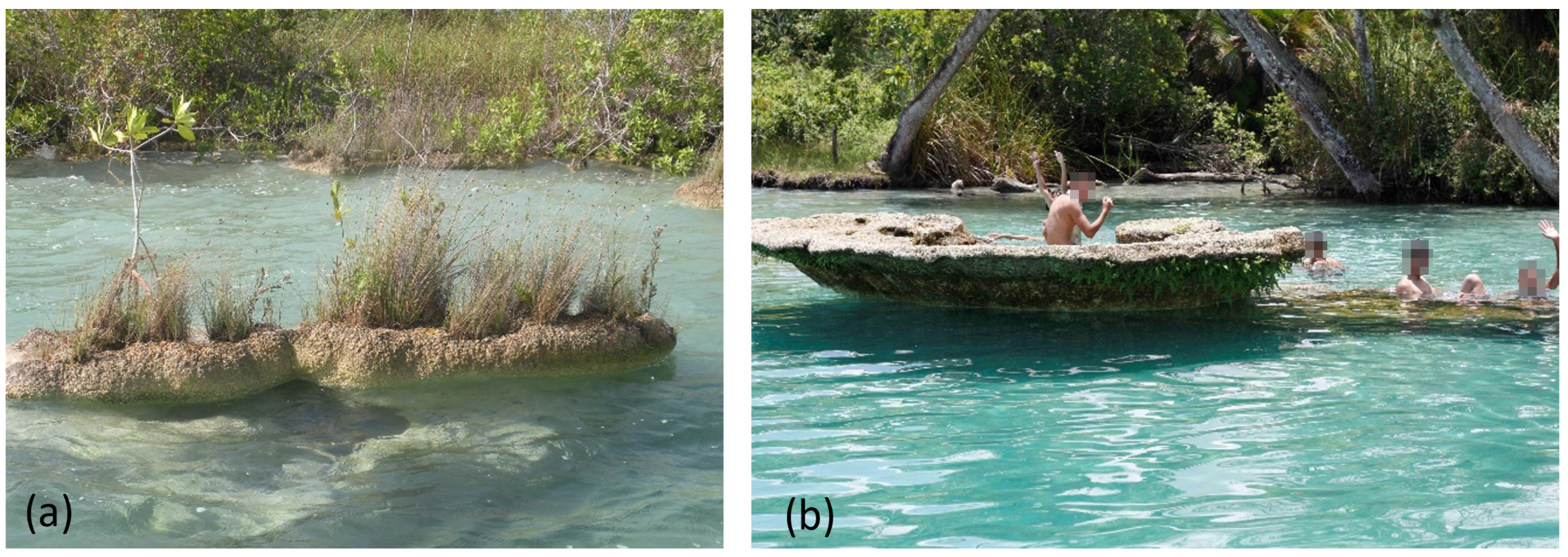
An oligotrophic water body with a high ecological value is the Bacalar Lagoon in Quintana Roo, Mexico, also known locally as Laguna de los 7 colores (Lake of Seven Colors). This lagoon has become an important tourist destination due to its ecological appeal and the presence of stromatolites, which are rock structures built by colonies of microscopic organisms known as cyanobacteria that do photosynthesis. Stromatolites are very important because they are evidence of the oldest known life on Earth and are part of the most important fossil record of early microbiological life [25]. The formation of stromatolites is as follows: once the soil settles in shallow water, cyanobacteria use water, carbon dioxide, and sunlight to create their food. Often, a layer of mucus forms over the cyanobacterial cell mats, joining the sedimentary particles and building additional layers until mounds are formed [26]. In Figure 1a, stromatolites from the Bacalar lagoon can be seen. Unfortunately, in recent years, anthropogenic contamination in this lagoon has progressively increased due to the discharge of untreated wastewater, deforestation, the use of fertilizers in agriculture, and the high tourist demand [27,28,29,30]. Therefore, in some seasons of the year, water with mesotrophic and eutrophic characteristics has been detected in some areas along its extension [31]. Although it has not been fully evaluated how stromatolites are being affected by contamination, it is known that variations in the physicochemical properties of water can affect its diversity, composition, and growth rates [32,33,34]. Additionally, they are also being directly affected by tourists due to ignorance and lack of adequate signs, as can be seen in Figure 1b. Therefore, the water monitoring of this lagoon has become a priority issue for the authorities and ecological groups of the Quintana Roo state.

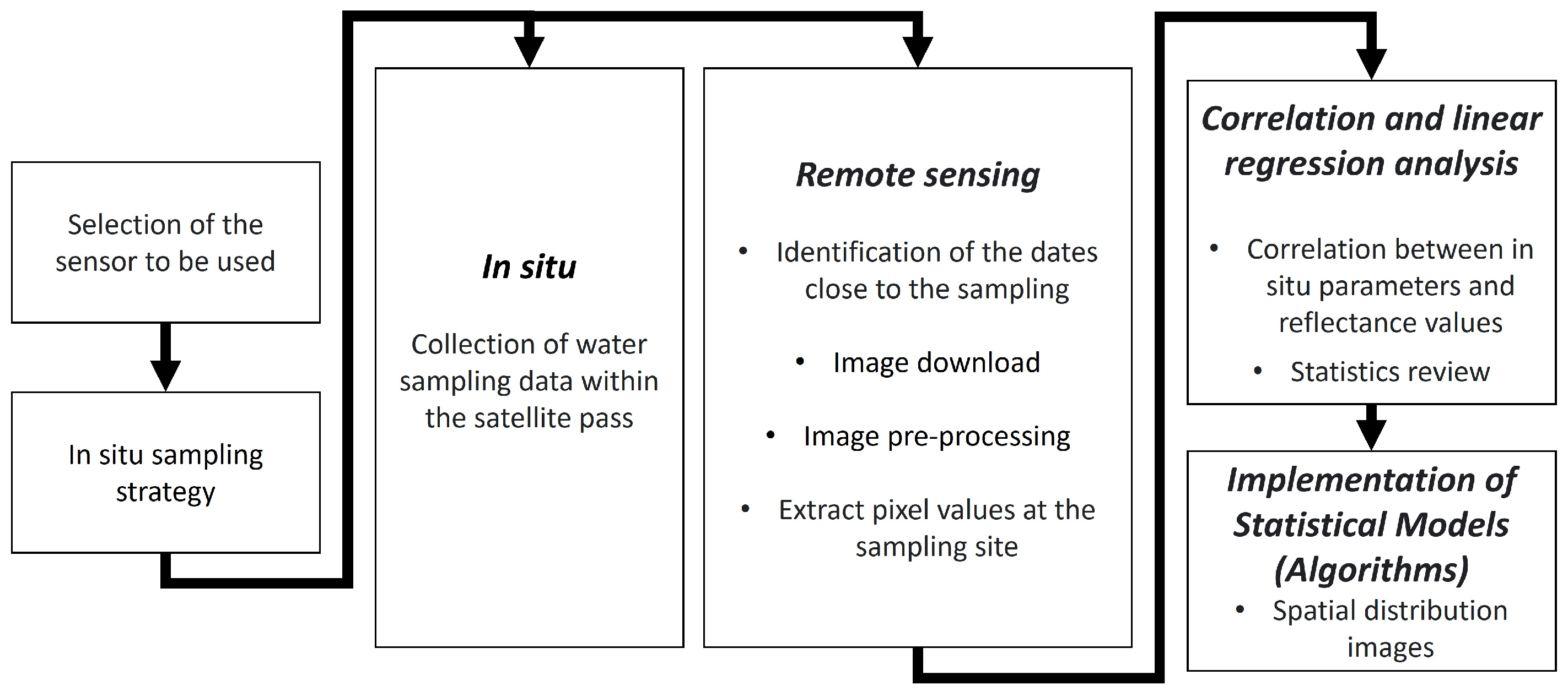
In order to contribute to conservation efforts in Bacalar Lagoon, in this work, we present a systematic study to predict the spatial variability of a set of six physicochemical parameters frequently used in water quality assessments [35]: dissolved oxygen (DO), total dissolved solids (TDS), oxidation–reduction potential (ORP), electrical conductivity (EC), salinity (S), and turbidity (Turb). This is achieved through correlation and linear regression analyses between in situ measurements of these parameters with remote sensing images from Landsat 8 and Sentinel 2 sensors. The results for EC, S, Turb, and TDS are in agreement with the values reported for this lagoon, highlighting the feasibility of using remote sensing tools to monitor oligotrophic water bodies.

2. Material and Methods

2.1. Study Area

The Bacalar hydrological system with extreme latitude and longitude coordinates (${18}^{\circ }{56}^{\prime }$ N, $-{88}^{\circ }{9}^{\prime }$ W) to (${18}^{\circ }{33}^{\prime }$ N, $-{88}^{\circ }{28}^{\prime }$ W) is located southeast of the state of Quintana Roo, Mexico. This system belongs to the hydrological region number 33 according to the classification of the National Water Commission [36] and is composed of the Bacalar Lagoon and several parallel minor lagoons: Chile Verde, Guerrero, Mariscal, Milagros, and La Sabana Lagoon. The extension of the Bacalar Lagoon is approximately 42 km long and 2 km at its widest, while its average depth is 8 m with a channel in the central part approximately 15 m deep [25,37]; see Figure 2. There are several sinkholes (known locally as cenotes) inside the lagoon (Cocalitos, Esmeralda, and Negro) and around the lagoon (Cenote Azul) with a direct connection to it. The south of the Bacalar Lagoon is known locally as the Xul-Ha Lagoon and has a sinkhole inside with a connection to groundwater [25,38,39].

The lagoon is located at the Bacalar fault system in the evaporite region of the Yucatán peninsula, which is characterized by relatively water-soluble rocks of low permeability that include gypsum, calcite, dolomite, and minerals, such as celestite (${\mathrm{SrSO}}_4$) [40]. Due to the rock dissolution, there is a high concentration of sulfates and calcium in the groundwater, which is manifested in some sections of the lagoon due to the connection and mixing of waters [38]. The rocks vary in age from Cretaceous to Holocene. The outcrops to the north are of marine Pliocene to Holocene ages; in the south, they belong to the Miocene, and along the west side of the lagoon, they are from the Upper Cretaceous [41]. In some areas, there are rocky shores, while towards the center and south of the lagoon, there are areas of shallow, fast-flowing water (rapids) with the presence of stromatolites, an almost unique natural treasure [25]. The flow circulation pattern within the lagoon is from south to north (Xul-Ha to the town of Bacalar) and from north to south, converging in the middle of the lagoon [34]. The topographic relief is from the south (higher elevations) to the north (lower elevations).

The climate in the region is tropical humid, with an average annual temperature of 26 °C. There are three dominant seasons: cold front rains (from October to April), dry season (between April to May), and tropical cyclones and hurricane season (from June to October). The average annual rainfall in the region ranges from 100 to 1500 mm [42].

2.2. Methodology

Figure 3 shows a flowchart with the research methodology followed in this work. The methodology can be split into four general parts once the satellite sensors have been selected: (1) water sampling, (2) remote sensing, (3) correlation and linear regression analysis, and (4) implementation of the statistical models (algorithms) to predict physicochemical parameters and their spatial distributions.

2.2.1. Satellite Image Selection

There is a wide variety of sensors installed on satellites with different spatial resolutions, which have been used intensively in water quality monitoring studies such as Landsat TM, Landsat ETM+, ASTER, MERIS, MODIS, and recently, the Sentinel family [43]. Some of these sensors have multispectral (mostly with 3 to 10 bands) or hyperspectral characteristics (50 bands or more).

Although multispectral data from remote sensors are used to analyze the quality of water in continental or marine water bodies, their fundamental limitation is the spectral resolution, which may influence efficiency depending on the period of time or study area, compared to hyperspectral sensors [16]. These latter types of sensors have continuous bands with a spectral resolution starting at 5 nm, which allows distinguishing differences in spectral mixing, improving accuracy in the interpretation of water quality parameters [44]. However, not all images from these sensors are free to access (at no cost), which limits the choice of images to use.

Currently, several works make use of multispectral data from Landsat 8 and Sentinel 2 to evaluate water quality and present favorable results for typical water quality parameters [24,45,46,47]. Taking into account the spatial, temporal, and spectral resolution and mainly the accessibility of the information from Landsat 8 and Sentinel 2 sensors, they are the most used in the assessment of water quality parameters [16]. Therefore, they were chosen to carry out the present study, and they are briefly described below.

The satellite Landsat 8 is widely used to obtain information using two scanning instruments: the Operational Land Imager (OLI) and the Thermal Infrared Sensor (TIRS). The spectral bands of the OLI sensor, although similar to the Landsat 7 ETM+ sensor, provide an improvement on the instruments of previous Landsat missions. This is due to the incorporation of two new spectral bands: a deep channel in the visible blue (band 1) designed specifically for the analysis of water resources and research in coastal areas and an infrared channel (band 9). The data quality and 16-bit radio-metric resolution of the OLI and TIRS are higher than in previous sensors (8 bits for TM and ETM+), providing a significant improvement in the ability to detect changes in the Earth’s surface [11,48].

On the other hand, Sentinel 2 is part of the European Space Agency (ESA). It has a temporal resolution of 10 days, with a spatial resolution between 10 and 60 meters, and has 13 spectral bands. In addition, its camera has two focal planes, the first in the visible (VIS) and near-infrared (NIR) bands and the second in the mid-infrared (SWIR) [49].

The images downloaded from Landsat 8 and Sentinel 2 are images of digital numbers with values between 0 and 255, so they require additional processing to convert them into irradiance or reflectance images.

2.2.2. Water Sampling

In October 2018, a water sampling campaign was carried out to measure physicochemical parameters of water quality, obtaining information at 71 points; 35 in the Xul-Ha lagoon, and 36 in an area near the town of Bacalar (from now on, we will refer to this place as the Bacalar Lagoon), as can be seen in Figure 2. The average separation between contiguous points was 200 m and was chosen based on the spatial resolution of the satellite images; 30 m per pixel for Landsat 8 and 10 m per pixel for Sentinel 2 (see dots in Figure 2). Furthermore, this separation allows to cover the maximum extent within the monitoring areas. For each point site, the following physicochemical parameters were evaluated: dissolved oxygen (DO, mg/L), total dissolved solids (TDS, g/L), oxidation–reduction potential (ORP, mV), electrical conductivity (EC, μS/cm), salinity (S, ppt), and turbidity (Turb, NTU), as previously mentioned. In addition, the percentage of dissolved oxygen (DO %) was considered. Parameter measurements were performed using a Hydrolab DS5 probe (OTT Hydromet GmbH, Kempten, Germany). For the EC parameter, a second measurement was obtained using a CTD Castaway (SonTek Xylem, San Diego, CA, USA), which was used in addition to measuring the temperature (T, °C) and pH of water. All measurements were taken at a depth of 1 m from the surface of the lagoon. It is important to mention that in the same year as the water sampling campaign, oligotrophic water conditions were reported at the site called Bacalar Lagoon, based on measurements from the years 2016 to 2017.

2.2.3. Remote Sensing

Two images were chosen: the first from Landsat 8 (OLI), which belongs to the scene Path 19/Row 47, and the second from Sentinel 2. The dates the images were obtained were Landsat 8, 12 September 2018, and Sentinel 2, 17 October 2018; both images had a time lag concerning the monitoring date. These lags, 34 days for OLI and 1 day for Sentinel, are within the standards recommended for remote sensing analysis of water bodies [50,51]. Due to the presence of clouds over the lagoon, an atmospheric correction process with a dark object subtraction model [52] was carried out using the AtmosC module of the TerrSet software (https://clarklabs.org/terrset/, accessed on 22 November 2023). This process generates an image of corrected digital numbers.

Reflectance images, which are required for the spectral analysis, were generated from the images of digital numbers for each band of each sensor used. The used bands of Landsat 8 and Sentinel 2 and their specifications are indicated in

Table 1. Band specification for sensors from Landsat 8 and Sentinel 2.

Landsat 8 (OLI)			Sentinel 2
Band	Spatial Resolution	Wavelength (μm)	Band	Spatial Resolution	Wavelength (nm)
Band 1 Coastal aerosol	30 m	$0.435–0.451$	Band 2 Blue	10 m	$0.440–0.530$
Band 2 Blue	30 m	$0.452–0.512$	Band 3 Green	10 m	$0.537–0.582$
Band 3 Green	30 m	$0.533–0.590$	Band 4 Red	10 m	$0.646–0.684$
Band 4 Red	30 m	$0.636–0.673$	Band 8 NIR	10 m	$0.760–0.908$
Band 5 Near-infrarred (NIR)	30 m	$0.851–0.879$
Band 6 SWIR-1	30 m	$1.566–1.651$
Band 7 SWIR-2	30 m	$2.107–2.294$
Band 10 TIRS-1	100 m	$10.60–11.19$
Band 11 TIRS-2	100 m	$11.50–12.51$

Note: data from references [48,49].

. The following equation was used to change from an image of digital numbers to another of reflectance values:

$${\rho }_{\lambda }^{\prime }=M_p·Q_{cal}+A_p,$$

(1)

where ${\rho }_{\lambda }^{\prime }$ is the atmospheric reflectance. $M_p$ and $A_p$ are the multiplicative and additive factors for the scale change for a specific band, and $Q_{cal}$ is the value of the digital number of the image, which already includes the atmospheric correction. The scale factors are part of the metadata files of the satellite images and are found with the specific names of reflectance_mult_band_x and reflectance_add_band_x, respectively, where x indicates the specific band. To compare images obtained in different seasons, it is necessary to consider the value of the solar angle, which is given by the following equation:

$${\rho }_{\lambda }={\rho }_{\lambda }^{\prime }/cos\left({\theta }_{SZ}\right)={\rho }_{\lambda }^{\prime }/sin\left({\theta }_{SE}\right),$$

(2)

where ${\rho }_{\lambda }$ is the total atmospheric reflectance, and ${\theta }_{SE}$ and ${\theta }_{SZ}$ are the angles of local elevation and solar zenith, respectively [48].

2.2.4. Correlation and Linear Regression Analysis

In general, there are a wide variety of methods that have been successfully applied for the analysis of water quality parameters, e.g., linear regression methods [53], nonlinear regression methods [54], multivariate models [55], neural networks [56], among many others. Although each parameter has a very specific behavior with respect to the light spectrum, it has been observed that applying linear models provides a good fit for the determination coefficient ($R^2$) for most of them, as confirmed for some parameters, such as Chlorophyll-a (Chl-a), Total Suspended Solids (TSS), pH, iron (Fe), zinc (Zn), chromium (Cr), and ammonium (NH4) [57,58,59]. Furthermore, nowadays, the linear regression method is the most used for the assessment of water quality parameters through remote sensing.

In fact, given the lack of information on remote sensing analysis in oligotrophic water bodies, in this work, we use as a first approximation the following linear methods to estimate the correlation between the reflectance images with the water data measured in the field: (1) simple correlation, (2) multiple correlation, and (3) correlation with ratios [53]. Before performing any analysis, it is necessary to generate a mask to extract valid pixels for each reflectance image, i.e., the only pixels used in the correlation analysis were those where there was a field measurement. Therefore, it is implicitly assumed as a valid approximation that in situ measurements are representative of areas of the size of the spatial resolution (pixel) of each image; that is, 10 m for Sentinel 2 and 30 m for Landsat 8 [14,19,60].

Simple correlation analysis, characterized by the Pearson correlation coefficient r, was performed for every physicochemical parameter for each band of each sensor (parameter vs. specific band), considering all valid pixels. In all cases, a simple linear regression (SLR), characterized by the coefficient of determination $R^2$, was carried out using the following equation:

$$y=a+b{x}_i,$$

(3)

where y (dependent variable) is the value of a physicochemical parameter sampled in situ, and $x_i$ (independent variable) is the reflectance value in the band i of the pixel associated with the coordinates of the sampling point. Constants a and b are fitting parameters. This type of analysis is used to verify the spectral response of each parameter at different wavelengths. Table 1 shows the wavelengths associated with each of the bands used for the Landsat 8 and Sentinel 2 sensors.

On the other hand, a multiple correlation analysis, characterized by the multiple correlation coefficient r, was carried out on a set of bands for each physicochemical parameter, which broadens the range of the light spectrum considered for each one. The multiple linear regression (MLR) [61], characterized by its coefficient of determination $R^2$, which was used for this case, is given by the following equation:

$$y=a+\sum _i{b}_i{x}_i,$$

(4)

where the sum runs over the number of bands chosen for each sensor (see Table 1). In this analysis, a linear relationship is assumed between the reflectance bands $x_i$ and the physicochemical parameter y. Constants a and $b_i$ are fitting parameters.

Finally, correlation and simple linear regression analysis were performed, but instead of using the reflectance value of a given band as the independent variable, several relationships between the reflectance bands (band ratios) were used. Correlations with ratios aim to extract more precise information from a required surface, in this case, the water body.

Table 2. Band ratios and scale values for the correlation and regression analysis with ratios.

Band Ratios	Algorithm	Remark
R1: Enhancement of the red band	$(\mathrm{Green}+\mathrm{Red})/2$	water has a (+) value
R2: Enhancement of the red band	$\mathrm{Green}/\mathrm{Red}$	water has a (+) value
R3: Enhancement of the red band	$\mathrm{Red}/\mathrm{Green}$	water has a (+) value
R4: Enhancement of the infrared band	$\mathrm{NIR}/\mathrm{Green}$	water has a (+) value
R5: Enhancement of the infrared band	$\mathrm{Red}/\mathrm{Green}+\mathrm{NIR}$	water has a (+) value
R6: Normalized Difference Water Index (NDWI)	$(\mathrm{Green}-\mathrm{NIR})/(\mathrm{Green}+\mathrm{NIR})$	water has a (+) value
R7: Modified Normalized Difference Water Index (MNDWI)	$(\mathrm{Green}-\mathrm{MIR})/(\mathrm{Green}+\mathrm{MIR})$	(+) value
R8: Water Ratio Index (WRI)	$(\mathrm{Green}+\mathrm{Red})/(\mathrm{NIR}+\mathrm{MIR})$	water has a value > 1
R9: Automated Water Extraction Index (AWEI)	$4(\mathrm{Green}-\mathrm{MIR})(0.25\mathrm{MIR}+2.75\mathrm{SWIR})$	water has a (+) value

shows the band ratios considered in this work.

3. Results and Discussion

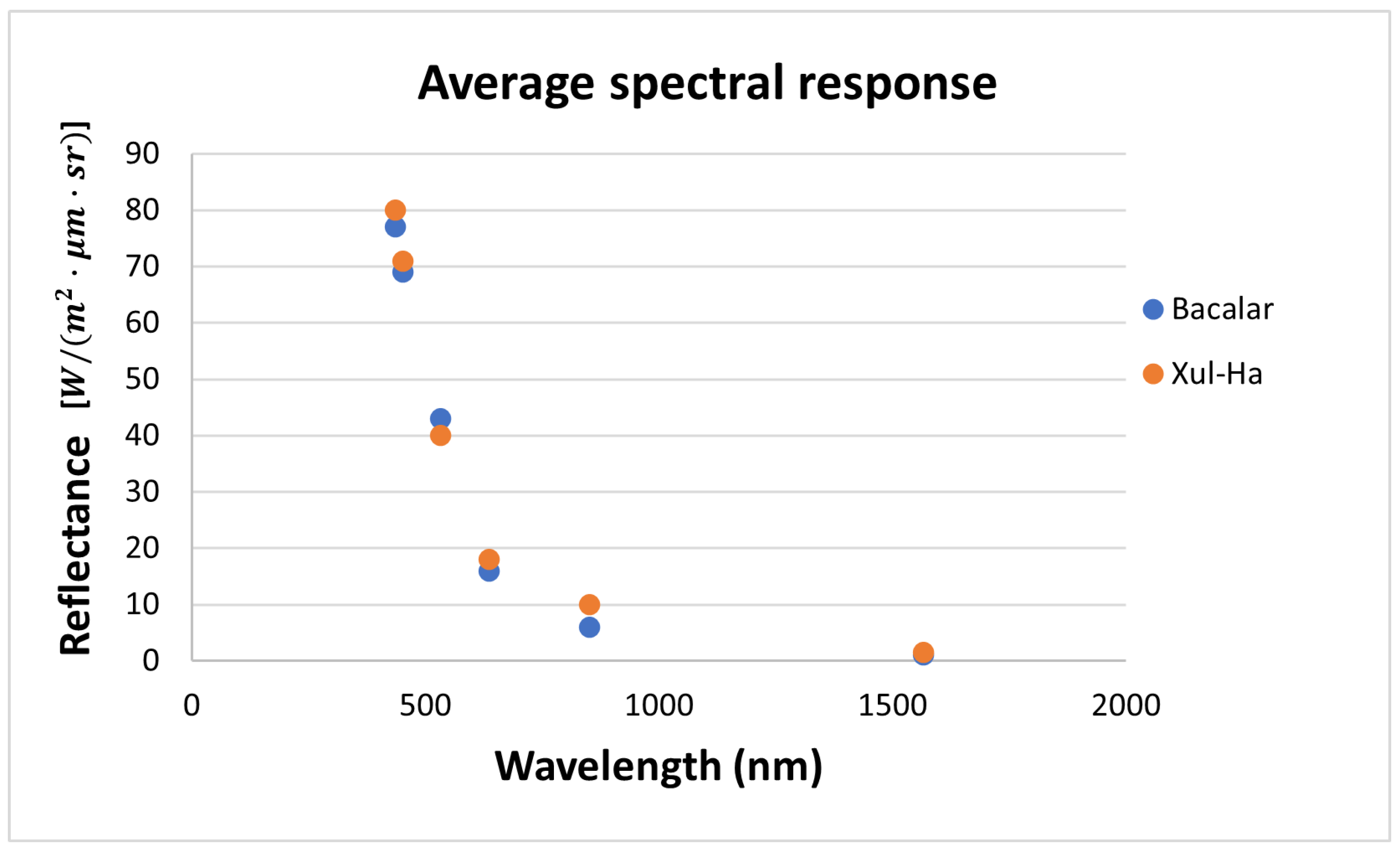
3.1. Average Spectral Response

From the point of view of the spectral response, the points evaluated in the Xul-Ha Lagoon behaved uniformly, unlike the points evaluated in the Bacalar Lagoon. This difference was more accentuated in the reflectances of the visible spectrum, which indicates that the penetration of light was different in Bacalar, mainly due to the different depths that occur in it. However, the average spectral response for both lagoons was similar, as can be seen in Figure 4. For this reason, all points from both study sites were considered as a single data set for the analysis of correlations and linear regressions, improving statistical representativeness.

3.2. Correlation and Linear Regression Analysis

Correlation and linear regression analyses were carried out using the individual bands, the sets of bands, and the band ratios for each physicochemical parameter considered. The correlation and determination coefficients obtained for each case can be seen in the tables in Appendix A.2.

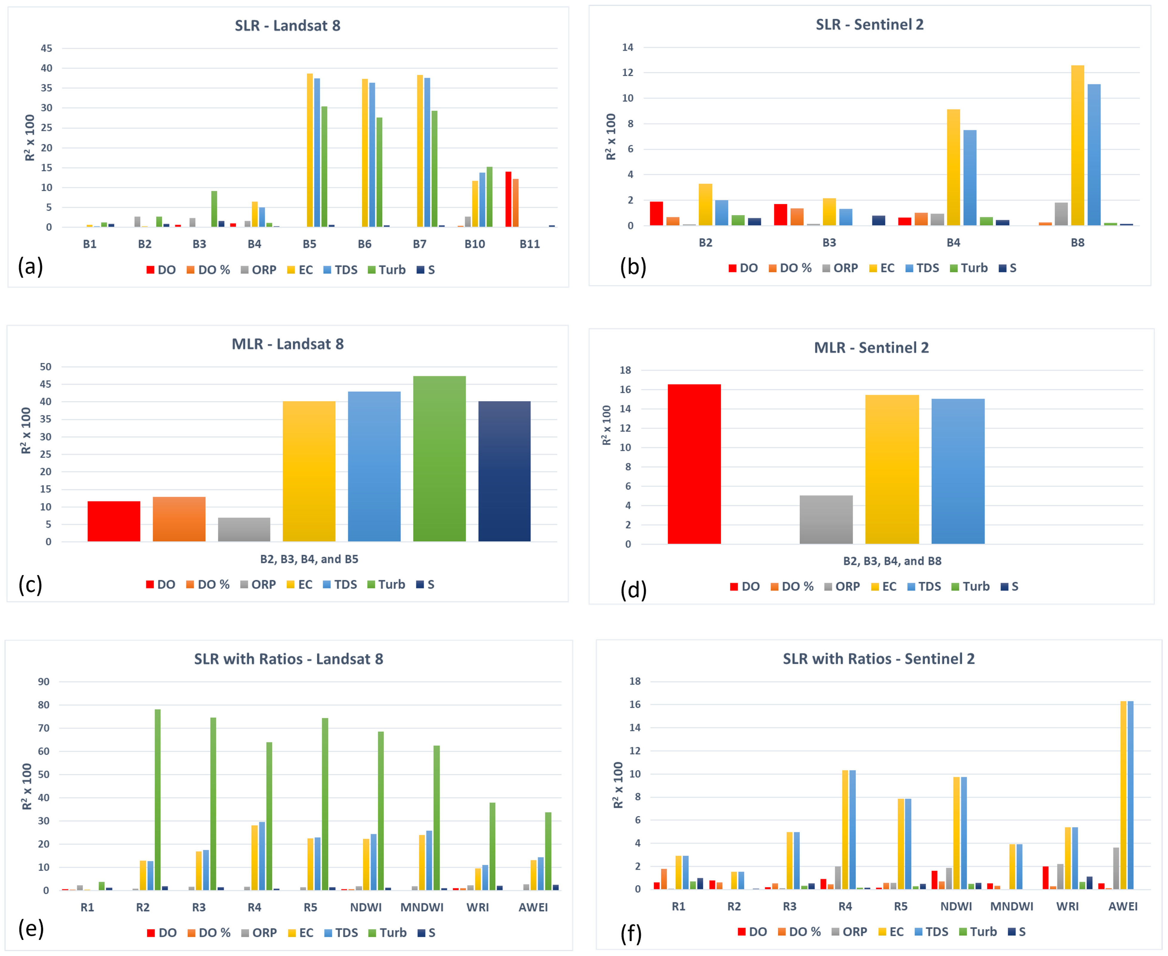
Figure 5a,b shows the coefficients of determination $R^2$ obtained from the SLR analysis on a percentage scale using the individual bands of the images Landsat 8 and Sentinel 2. It is observed that, for the Landsat 8 image, the maximum values of the coefficient of determination are presented in the near, mid, and far infrared bands, i.e., in bands 5, 6, and 7, respectively. These results contrast with those reported in [14], where it is mentioned that the ideal reflectance values for the water surface are greater in the visible spectrum range and disappear in the infrared range, just when the absorbance is higher. However, in that study, the analysis was carried out in water with eutrophic characteristics, where the spectral response can be very different from the response of water with or close to oligotrophic characteristics. For the SLR analysis using the Sentinel 2 image, only the bands with the highest spatial resolution (bands 2, 3, 4, and 8) were used. The behavior in the bands was similar to those obtained with the Landsat 8 image, although the $R^2$ values obtained with Sentinel 2 are lower than those obtained with Landsat 8. For the latter, $R^2$ values close to $0.40$ are obtained (bands 5 to 7), while for Sentinel 2 a maximum value of $0.12$ is obtained in the near-infrared band (band 8).

The fact that the linear regressions obtained with Sentinel 2 have a lower $R^2$ coefficient can be explained in terms of the spatial resolution of each image. The Sentinel 2 image has a higher spatial resolution (10 m), so the pixels evaluated can be very specific in terms of the surface they represent, while the Landsat 8 image has a lower spatial resolution (30 m), so their reflectances are average values that can include various surface types. On the other hand, the spectrum range occupied by each of the bands in each sensor is different. For Landsat 8 the bands of the visible spectrum are broader, while the spectral resolution for Sentinel 2 is lower and more specific, mainly in the green and red ranges. Regardless of the image used, it can be observed that for the SLR analysis, the maximum values of $R^2$ are given for the physicochemical parameters EC and TDS, which present a high correlation between them due to a close relationship from the chemical point of view [62]. In addition, both parameters are indicators of the salinity level of the water.

On the other hand, Figure 5c,d shows the coefficients of determination $R^2$ obtained from the MLR analysis. For each analysis, the spectrum bands that have the highest reflectance values in the water spectral signature were selected, that is, bands 2 (blue), 3 (green), 4 (red), and 5 (NIR) for Landsat 8, and bands 2 (blue), 3 (Green), 4 (red) and 8 (NIR) for Sentinel 2. Using the Landsat 8 image, the parameters that obtained the highest correlation were Turb, TDS, S, and EC, while for the Sentinel 2 image, they were DO, EC, and TDS. However, the last coefficients were lower than those obtained with the Landsat 8 image, similar to the results obtained from the SLR analysis. It is important to note that, for the Landsat 8 image, a better correlation for salinity was obtained with the MLR analysis than with the SLR analysis. Similarly, for the Sentinel 2 image, a better correlation was obtained for dissolved oxygen using the MLR analysis.

The $R^2$ values for the SLR with ratios can be seen in Figure 5e,f. The maximum value of $R^2$ (≈0.8) was obtained for the parameter Turb, using the band ratio R2 (Green/Red) and the Landsat 8 image. Therefore, it can be inferred that this parameter affects the parameters TDS, EC, and S in a complex way. Except for the band ratio R1, all ratios highlighted the parameter Turb, as well as TDS and EC, although the latter with $R^2$ values less than $0.30$. It can also be observed that in the band ratios where infrared spectrum bands were used (NDWI, MNDWI, WRI, and AWEI), the $R^2$ values were below the maximum $R^2$ obtained with the band ratio R2. The above contrasts with the results reported in [63], where it is indicated that the NDWI ratio could be used to detect subtle water variations.

Finally, it can be observed that the highest values of the coefficient of determination for all parameters were obtained with the MLR analysis, except for the parameter Turb, which had the highest $R^2$ using SLR with the band ratio R2.

3.3. Final Regression Algorithms

Based on the analysis in the previous section, the statistical models (algorithms) that were significant and presented the highest values of the coefficient of determination $R^2$ were selected for each of the physicochemical parameters considered. The best algorithms were obtained with the Landsat 8 image. The final regression algorithms used to generate the spatial distribution of each parameter are presented in

Table 3. Statistical models to estimate physicochemical parameters of water quality.

Parameter	${\mathit{R}}^2$	Regression Type	Algorithm
DO	11.614	MLR	$DO=7.763192-68.169971·B2+4.695524·B3+140.907383·B4-34.471720·B5$
DO %	12.909	MLR	$DO\%=103.179877-939.421364·B2+90.563581·B3+1853.595989·B4-466.516875·B5$
ORP	6.937	MLR	$ORP=155.184756-1185.226496·B2+505.712058·B3+480.055127·B4+66.895446·B5$
EC	40.202	MLR	$EC=2677.194141-3489.917091·B2+2390.533199·B3+2357.910294·B4-8350.462172·B5$
TDS	42.915	MLR	$TDS=1.668721-1.446831·B2+0.910117·B3+1.990372·B4-5.362842·B5$
Turb	78.234	SLR-ratios	$Turb=-0.714183+17.342056·R2$
S	40.220	MLR	$S=1.435570-1.626862·B2+1.138029·B3+1.194380·B4-4.577200·B5$

.

It is important to mention that no images were generated for dissolved oxygen in the two forms evaluated nor for the oxidation–reduction potential since their $R^2$ values were less than $13\%$, which is considered a low value to use the regression algorithms to predict spatial distributions from the reflectance images. Although the Bacalar lagoon system is wider in extent, the resulting images are limited to the study area without the presence of clouds, despite the analysis carried out to filter them. This is because the filtering process modifies the real reflectances in cloud-covered pixels, so they should not be used to estimate the physicochemical variables in the prediction processes.

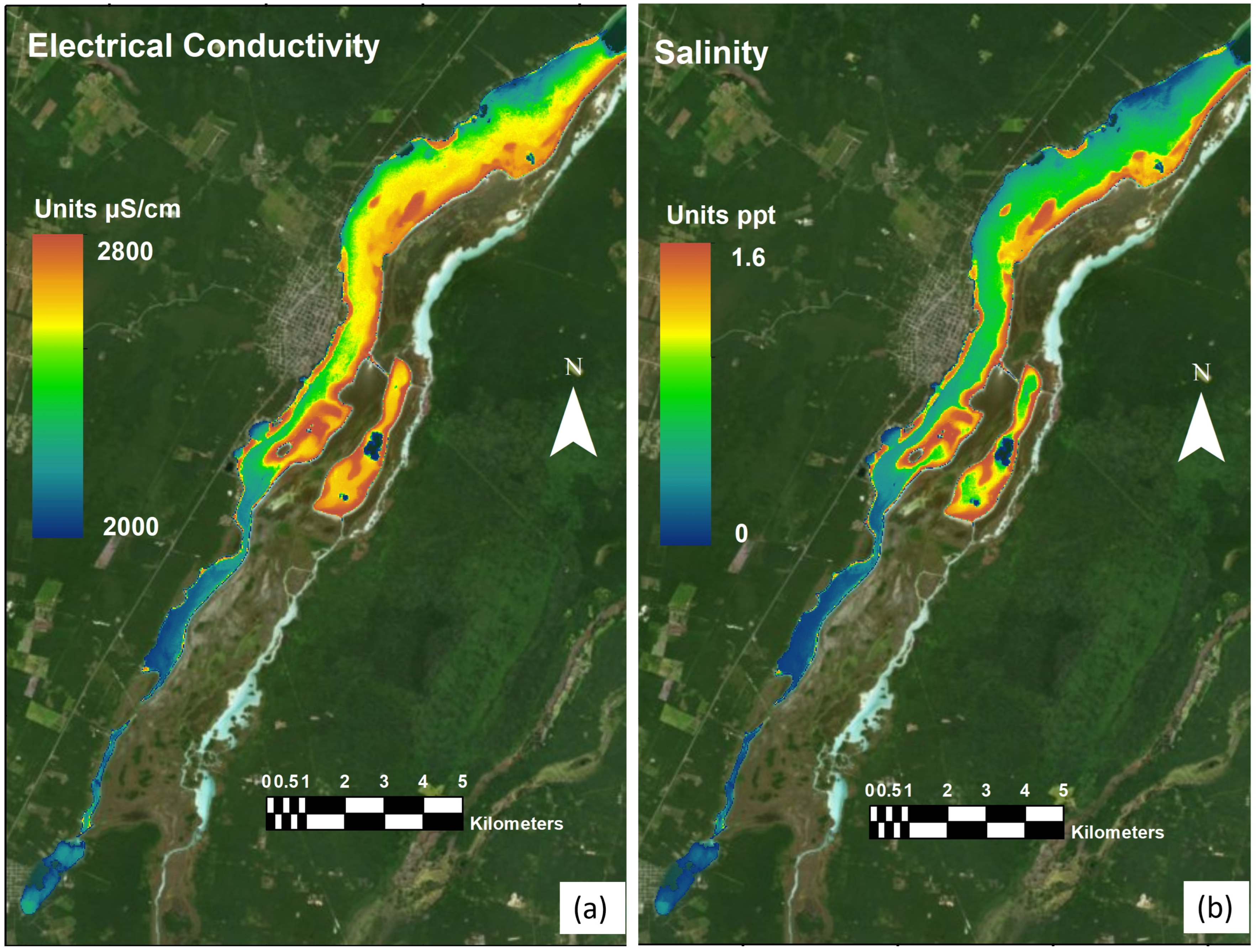
Figure 6 shows the spatial distributions of electrical conductivity and salinity. It can be observed that in the region near the town of Bacalar, on the west side of the lagoon, the values of the electrical conductivity EC are smaller than on the east side. Likewise, they decrease from north to south in the direction of Xul-ha Lagoon. This behavior has already been described previously [38] and is because the lagoon is shallower in the eastern part than in the western part. The shallow depth of the lagoon promotes higher evaporation, increasing salinity S and, consequently, the EC values. Similarly to the north of the lagoon, there is less interaction with groundwater than to the south of the lagoon, which explains the decrease in the EC parameter from north to south. Furthermore, it can be seen that the generated EC image is similar to the S image, indicating a high correlation between both parameters.

The average EC and pH values of the water, obtained from the in situ measurements, were $2479.66$ $\mathsf{\mu }$S/cm and $7.85$, respectively (see Appendix A.1)—similar to values previously reported in this lagoon [25,30,33,38], and in the range of values reported for water bodies with oligotrophic characteristics [38]. Another work with comparable results is the one reported in [64], in the area known as Los Rápidos (The Rapids), where an EC of 1220 $\mathsf{\mu }$S/cm was reported. In the case of the EC prediction map, the value obtained for the area is around 2000 $\mathsf{\mu }$S/cm.

Although the degree of water eutrophication involves measuring total phosphorus, nitrogen, and chlorophyll [65], from the spatial values of EC and pH, it can be inferred that at the time of measurements, the Bacalar lagoon presented oligotrophic conditions in most of its extension, mainly towards the south of the lagoon, decreasing slightly towards its northern section. However, this condition has changed over time, and punctual eutrophication has occurred temporarily in some areas along this lagoon [31].

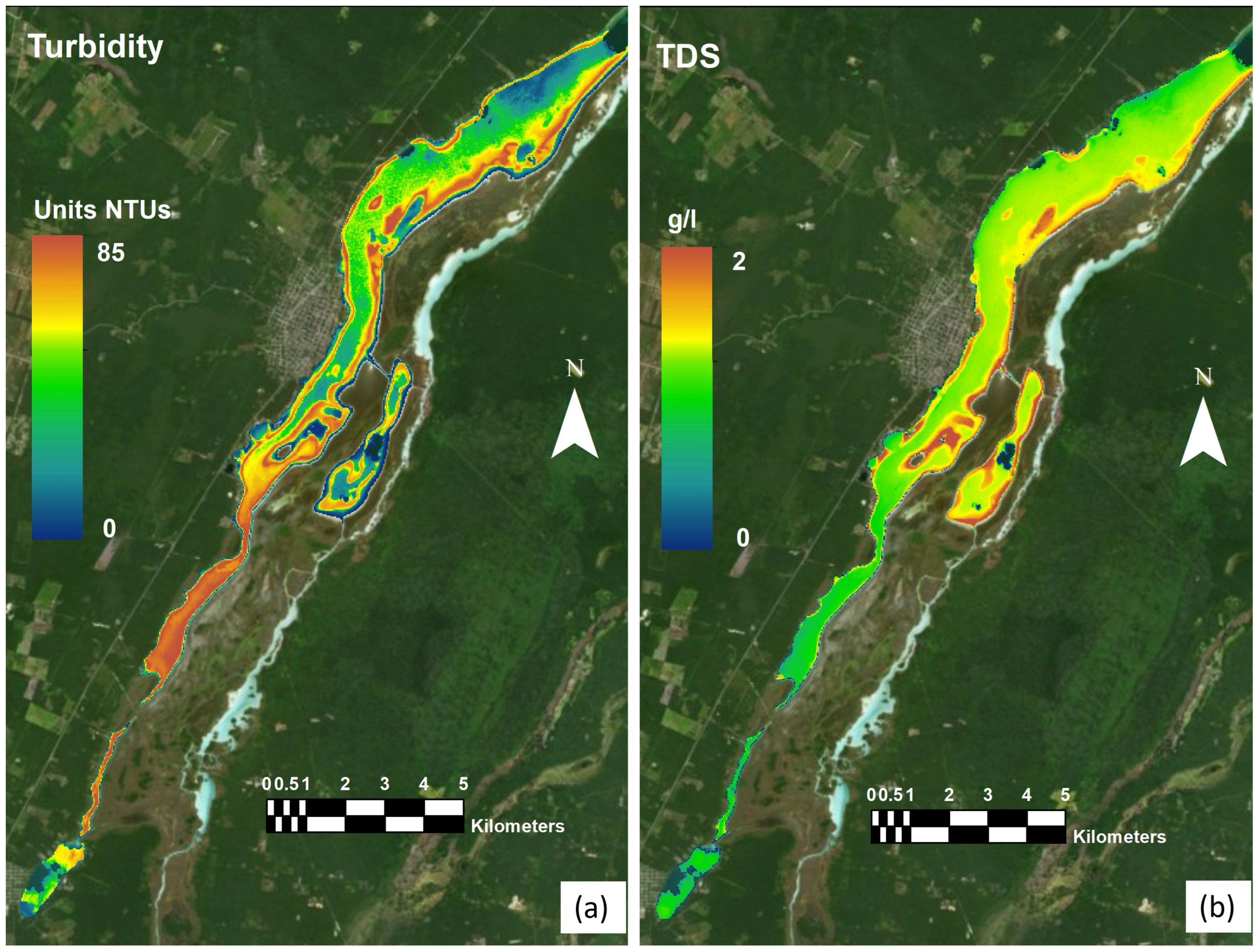
On the other hand, Figure 7 shows the spatial distributions of turbidity and total dissolved solids, which are considered aesthetic parameters of water. Turb is not a parameter regulated by the Official Mexican Standard (NOM-001-SEMARNAT-2021) [66]; however, it is one of the most important factors that restrict the growth of stromatolites [67]. As can be seen from this figure, the highest turbidity values occur in the narrowest section of the lagoon, to the south of it, before and after Los Rápidos. Stromatolites are found at this site, which may be affected due to the estimated concentrations of this parameter (85 NTUs). Likewise, high Turb values are found to the north of the lagoon, in its eastern section. It is important to emphasize that this parameter was best estimated using the SLR analysis with the R2 ratio (green/red). This result agrees with the statements that indicate that the spectral signature of the properties within the turbidity presents higher reflectance values in the spectrum ranging from 400 nm to 800 nm (this interval covers the green and red wavelengths, as can be seen in Table 1).

Concerning the TDS, the average value obtained from field measurements was $1.6$ g/L. It can be observed that the TDS values obtained in the western part of the lagoon, near the town of Bacalar, are similar to those reported in other studies in the same area [30,68] and are close to or above the limits allowed by current Mexican regulations [66,68].

In general, we can observe that the linear statistical models obtained reproduce, from a qualitative point of view, measurements reported for the parameters EC, S, Turb and TDS in various sites of the lagoon. However, it would be important to conduct more studies that consider more sophisticated models, and other satellite images with hyperspectral characteristics, to obtain better adjustments to the spatial behavior of these and other physicochemical parameters of the lagoon water.

It is important to mention that although the parameter data obtained in situ are representative of the period in which they were measured, they are similar to those reported in other years and different seasons of the year. This is due to the almost oligotrophic conditions of the lagoon that cause little temporal variability in the monitored data. However, it must be considered that the dynamics within the lagoon could be an important factor that modifies the results. In the case of Bacalar, monitoring in the months when extreme weather phenomena occur, e.g., in the cyclone and hurricane season, would be of vital importance since these phenomena alter the dynamics and composition of surface and groundwaters.

Regarding human activities, due to the accelerated increase in population in coastal areas, there is an urgent need for new and more cost-efficient methods for spatially explicit monitoring approaches at peatlands. For a better understanding of the ecological and hydrological behavior of the Bacalar Lagoon, remote sensing allows the generation of specific monitoring parameters due to the increase in human activities that will affect the fragile conditions of the lagoon and the stromatolites that reside in it, enabling rapid countermeasures to mitigate or minimize potential harm or hazard and even to decide if recurrent monitoring becomes necessary.

4. Conclusions

From the analysis of correlation and linear regression between images obtained from Landsat 8 and Sentinel 2 sensors, with field measurements of a set of physicochemical parameters, the statistical models that best represent the spatial behavior of the EC, S, Turb, and TDS in the Bacalar Lagoon were obtained.

Except for the Turb parameter, the most accurate algorithms were obtained using the Landsat 8 image and MLR analysis, which covers and considers a broader range of the electromagnetic spectrum. The set of parameters measured in the field allowed for an indirect analysis of the water quality of this lagoon, finding that at the time of the measurements, oligotrophic conditions were present in most of its extension.

From a general point of view, the results obtained demonstrate the feasibility of using remote sensing tools to frequently monitor large water bodies susceptible to contamination at a low cost compared to laboratory analysis.