
Analysis of Extreme Rainfall Characteristics in 2022 and Projection of Extreme Rainfall Based on Climate Change Scenarios


Abstract
:1. Introduction
2. Data and Method
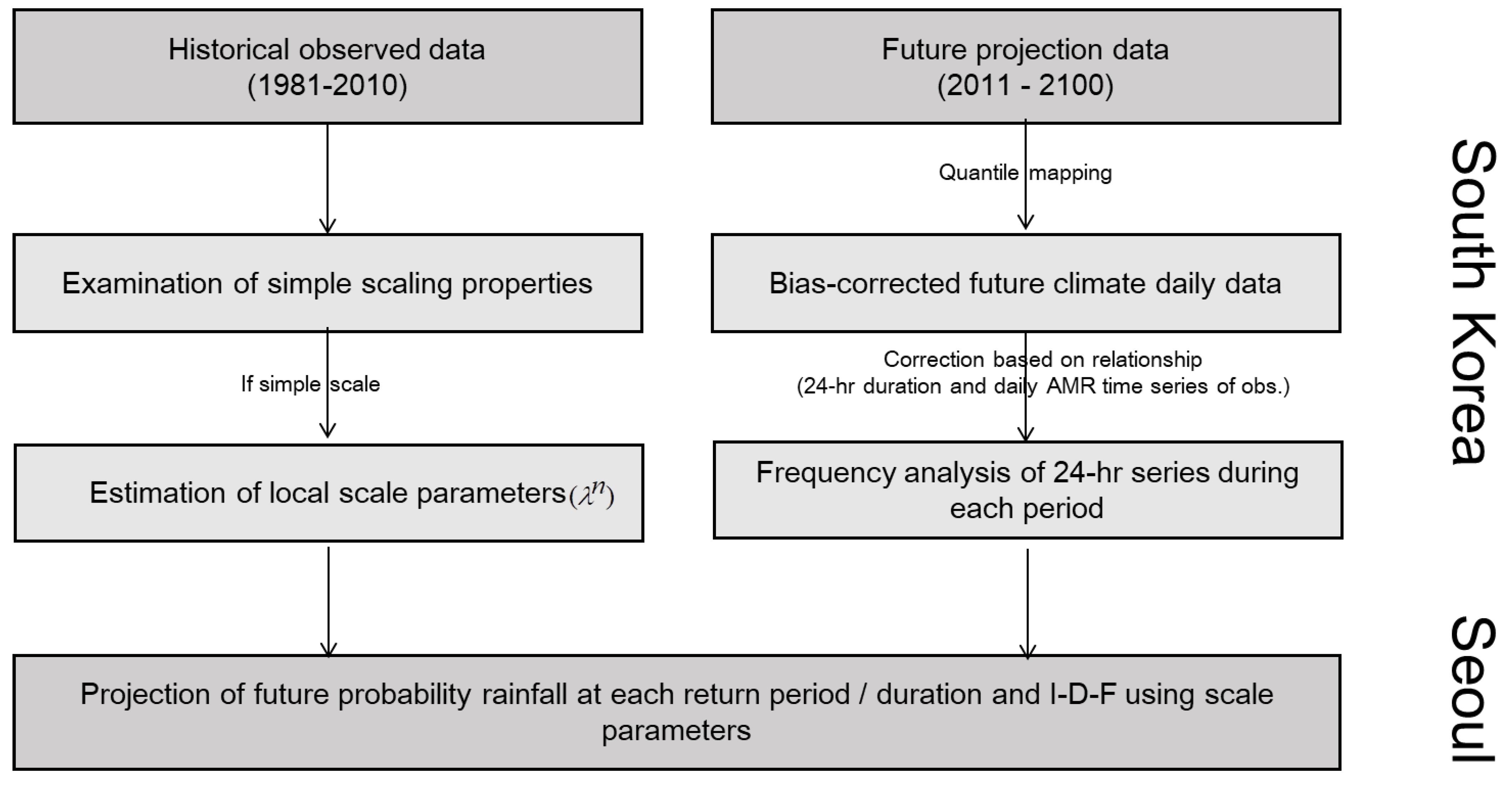
2.1. Method
2.2. Data and Methodology
2.2.1. Climate Change Scenarios
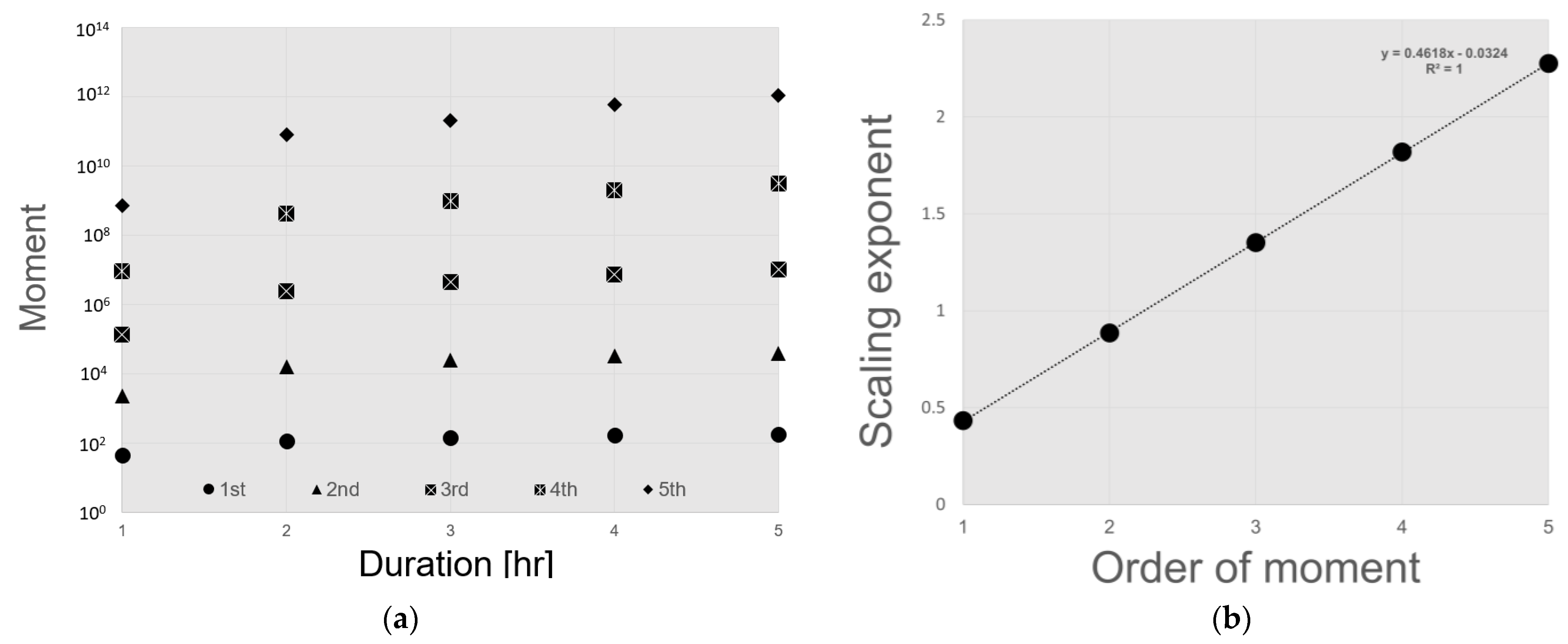
2.2.2. Calculation of Intensity–Duration–Frequency (IDF) Using the Scaling-Generalized Extreme Value (GEV) Distribution Model
3. Result
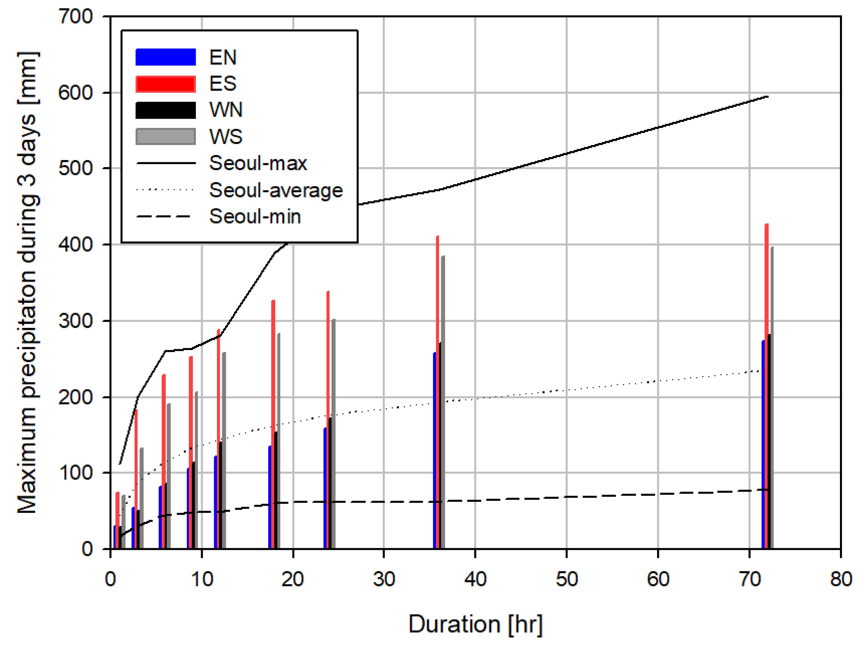
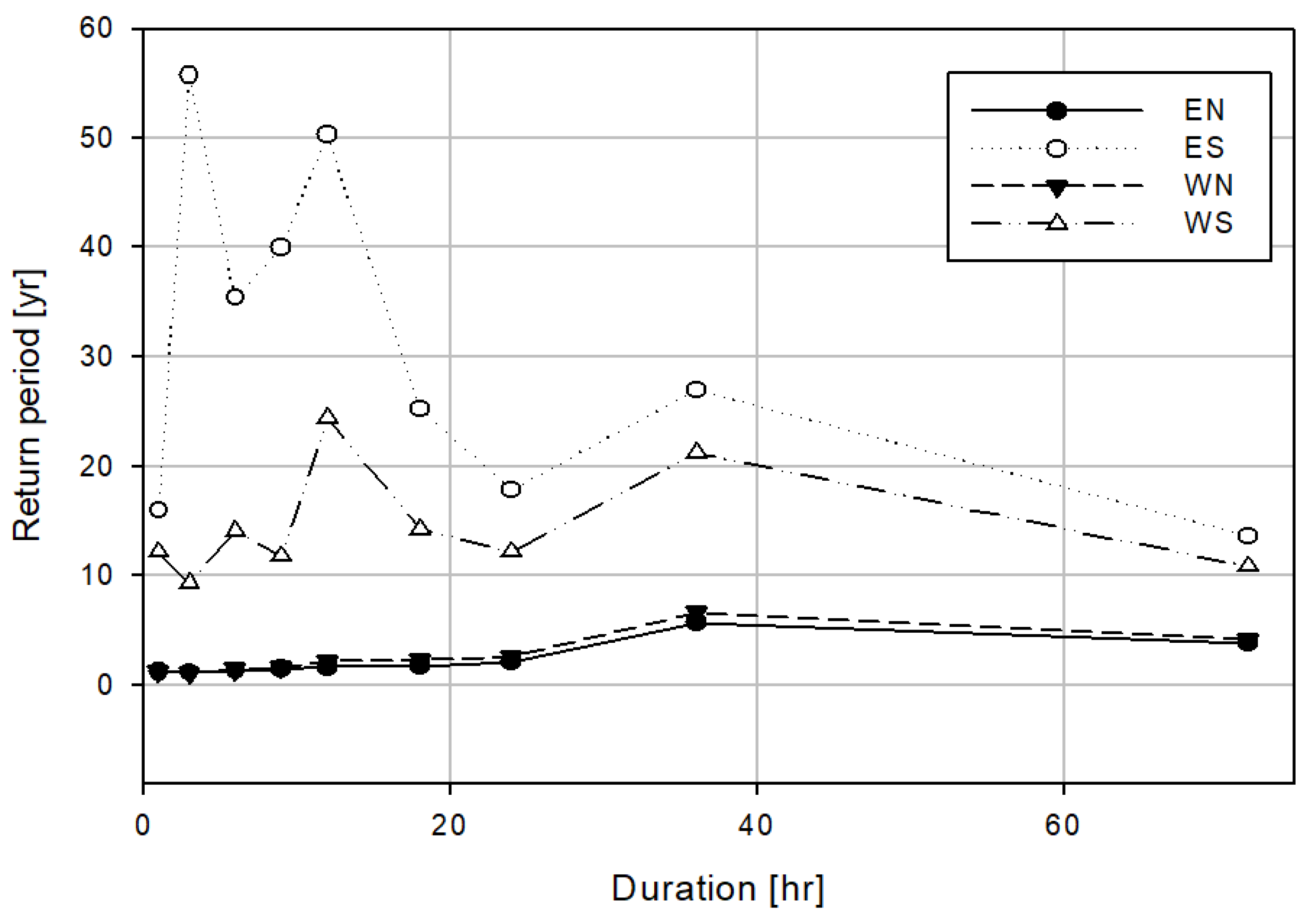
3.1. Characteristics of Heavy Rainfall That Occurred in Seoul in 2022
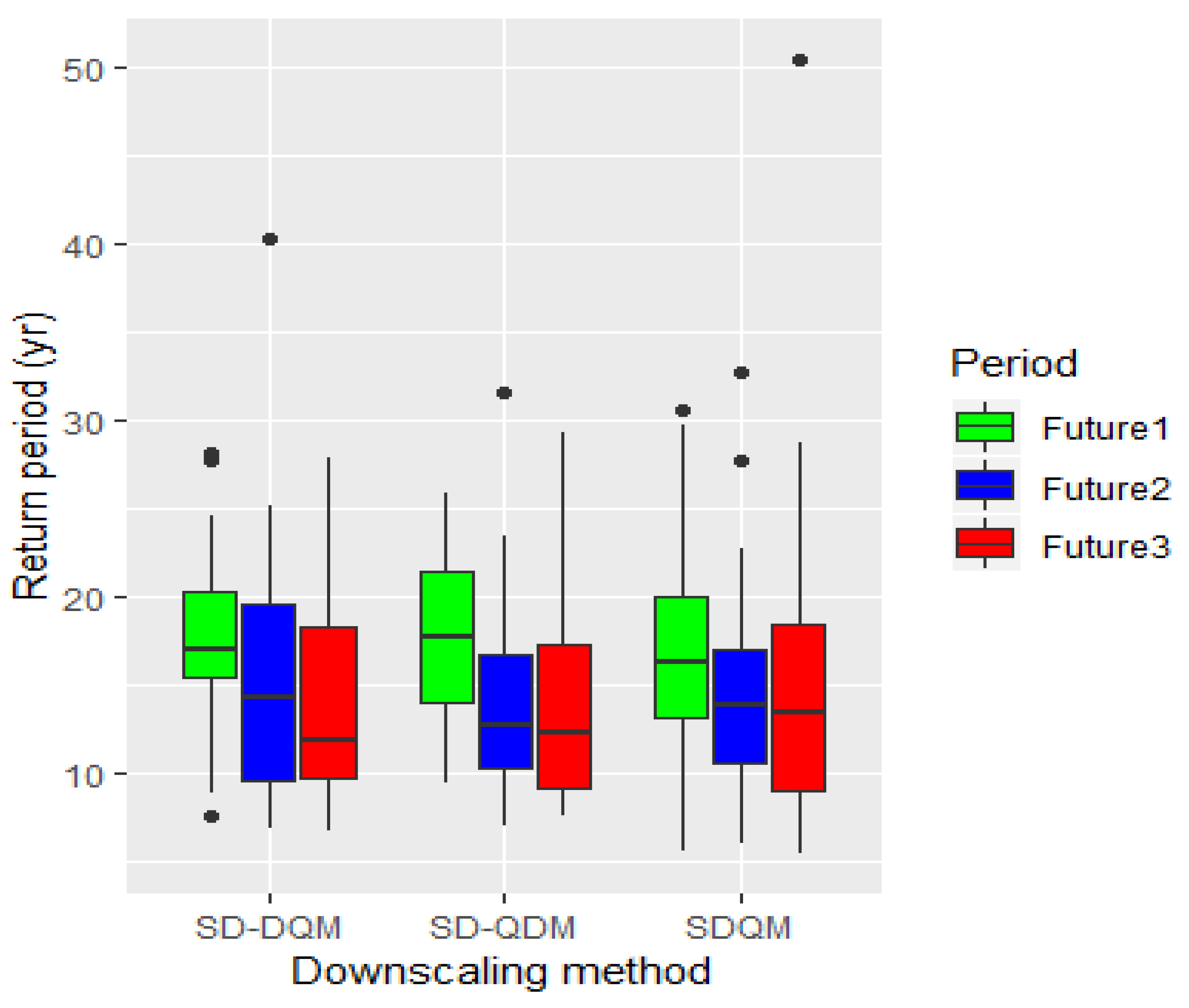
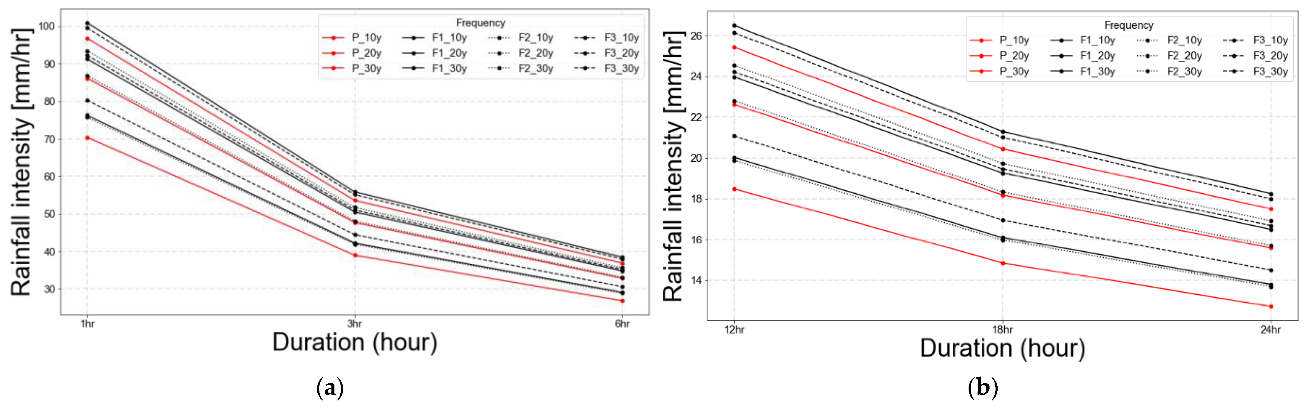
3.2. Projection of Future Intensity–Duration–Frequency (IDF) for SSP245
4. Conclusions
5. Discussion
Author Contributions
Funding
Data Availability Statement
Conflicts of Interest
References
- Min, S.-K.; Zhang, X.; Zwiers, F.W.; Hegerl, G.C. Human contribution to more-intense precipitation extremes. Nature 2011, 470, 378–381. [Google Scholar] [CrossRef]
- Westra, S.; Fowler, H.J.; Evans, J.P.; Alexander, L.V.; Berg, P.; Johnson, F.; Kendon, E.J.; Lenderink, G.; Roberts, N.M. Future changes to the intensity and frequency of short-duration extreme rainfall. Rev Geophys. 2014, 52, 522–555. [Google Scholar] [CrossRef]
- Milly, P.C.D.; Betancourt, J.; Falkenmark, M.; Hirsch, R.M.; Kundzewicz, Z.W.; Lettenmaier, D.P.; Stouffer, R.J. Stationarity is dead: Whither water management? Science 2008, 319, 573–574. [Google Scholar] [CrossRef]
- Kendon, E.J.; Stratton, R.A.; Tucker, S.; Marsham, J.H.; Bethou, S.; Rowell, D.P.; Sejior, C.A. Enhanced future changes in wet and dry extremes over Africa at convection-permitting scale. Nat. Commun. 2019, 10, 1794. [Google Scholar] [CrossRef]
- Martel, J.L.; Brissette, F.P.; Lucas-Picher, P.; Troin, M.; Arsenault, R. Climate Change and Rainfall Intensity-Duration-Frecuency Curves: Overview of Science and Guidelines for Adaptation. J. Hydrol. Eng. 2021, 26, 03121001. [Google Scholar] [CrossRef]
- Buonomo, E.; Jones, E.; Huntingford, C.; Hammaford, J. On the robustness of changes in extreme precipitation over Europe from two high resolution climate change simulations. Q. J. R. Meteorol. Soc. 2007, 133, 65–81. [Google Scholar] [CrossRef]
- Kwon, M.; Sung, J.-H.; Ahn, J. Change in extreme precipitation over North Korea using multiple climate change scenarios. Water 2019, 11, 270. [Google Scholar] [CrossRef]
- Nguyen, V.; Desramaut, N.; Nguyen, T. Estimation of urban design storms in consideration of GCM-based climate change scenarios. In Proceedings of the International Conference on Water & Urban Development Paradigms: Towards an Integration of Engineering, Design and Management Approaches, Leuven, Belgium, 15–17 September 2008; pp. 347–356. [Google Scholar]
- Vu, M.; Raghavan, S.; Liu, J.; Liong, S.Y. Constructing short-duration IDF curves using coupled dynamical–statistical approach to assess climate change impacts. Int. J. Climatol. 2018, 38, 2662–2671. [Google Scholar] [CrossRef]
- Choi, J.; Lee, O.; Jang, J.; Jang, S.; Kim, S. Future intensity–depth–frequency curves estimation in Korea under representative concentration pathway scenarios of fifth assessment report using scale-invariance method. Int. J. Climatol. 2019, 39, 887–900. [Google Scholar] [CrossRef]
- Yeo, M.-H.; Nguyen VT, V.; Kpodonu, T.A. Characterizing extreme rainfalls and constructing confidence intervals for IDF curves using Scaling-GEV distribution model. Int. J. Climatol. 2021, 41, 456–468. [Google Scholar] [CrossRef]
- O’Neill, B.C.; Krigler, E.; Rhiahi, K.; Ebi, K.L.; Hallegatte, S.; Carter, T.R.; Mathur, R.; van Vuuren, D.P. A new scenario framework for climate change research: The concept of shared socioeconomic pathways. Clim. Chang. 2014, 122, 387–400. [Google Scholar] [CrossRef]
- Song, Y.-H.; Chung, E.-S.; Shiru, M.S. Uncertainty analysis of monthly precipitation in GCMs using multiple bias correction methods under different RCPs. Sustainability 2020, 12, 7508. [Google Scholar] [CrossRef]
- Homsi, R.; Shiru, M.S.; Shahid, S.; Ismail, T.; Harun, S.B.; Al-Ansari, N.; Chau, K.W.; Yaseen, Z.M. Precipitation projection using a CMIP5 GCM ensemble model: A regional investigation of Syria. Eng. Appl. Comput. Fluid Mech. 2020, 14, 90–106. [Google Scholar] [CrossRef]
- Pierce, D.W.; Cayan, D.R.; Maurer, E.P.; Abatzoglou, J.T.; Hegewisch, K.C. Improved bias correction techniques for hydrological simulations of climate change. J. Hydromet. 2015, 16, 2421–2442. [Google Scholar] [CrossRef]
- Maraun, D. Bias correction, quantile mapping, and downscaling: Revisiting the inflation issue. J. Clim. 2013, 26, 2137–2143. [Google Scholar] [CrossRef]
- John, J.G.; Blanton, C.; McHugh, C.; Radhakrishnan, A.; Rand, K.; Vahlenkamp, H.; Wilson, C.; Zadeh, N.T.; Dunne, J.P.; Dussin, R. NOAA-GFDL GFDL-ESM4 Model Output Prepared for CMIP6 ScenarioMIP; Version 20180701; Earth System Grid Federation: Greenbelt, MD, USA, 2018.
- Yukimoto, S.; Kawai, H.; Koshiro, T.; Oshima, N.; Yoshida, K.; Urakawa, S.; Tsujino, H.; Deushi, M.; Tanaka, T.; Hosaka, M. The meteorological research institute earth system model version 2.0, MRI-ESM2.0: Description and basic evaluation of the physical component. J. Meteorol. Soc. Jpn. Ser. II 2019, 97, 931–965. [Google Scholar] [CrossRef]
- Voldoire, A.; Saint-Martin, D.; Sénési, S.; Decharme, B.; Alias, A.; Chevallier, M.; Colin, J.; Guérémy, J.F.; Michou, M.; Moine, M.P. Evaluation of CMIP6 DECK Experiments With CNRM-CM6-1. J. Adv. Model Earth Syst. 2019, 11, 2177–2213. [Google Scholar] [CrossRef]
- Seferian, R.; Nabat, P.; Michou, M.; Saint-Martin, D.; Voldoire, A.; Colin, J.; Decharme, B.; Delire, C.; Berthet, S.; Chevallier, M.; et al. Evaluation of CNRM Earth System Model, CNRM-ESM2-1: Role of Earth System Processes in Present-Day and Future Climate. J. Adv. Model. Earth Syst. 2019, 11, 4182–4227. [Google Scholar] [CrossRef]
- Boucher, O.; Denvil, S.; Levavasseur, G.; Cozic, A.; Caubel, A.; Foujols, M.A.; Khodri, M.; Krinner, G.; Lebas, N.; Levavasseur, G.; et al. IPSL IPSL-CM6A-LR model output prepared for CMIP6 CMIP historical. Earth System Grid Federation. J. Adv. Model. Earth Syst. 2018, 12, e2019MS002010. [Google Scholar] [CrossRef]
- Schupfner, M.; Wieners, K.H.; Wachsmann, F.; Steger, C.; Bittner, M.; Jungclaus, J.; Früh, B.; Pankatz, K.; Giorgetta, M.; Reick, C. DKRZ MPI-ESM1. 2-HR Model Output Prepared for CMIP6 ScenarioMIP; Version 20190710; Earth System Grid Federation: Greenbelt, MD, USA, 2019.
- Sellar, A.A.; Jones, C.G.; Mulcahy, J.P.; Tang, Y.; Yool, A.; Wiltshire, A.; O’Connor, F.M.; Stringer, M.; Hill, R.; Palmieri, J.; et al. UKESM1: Description and Evaluation of the U.K. Earth System Model. J. Adv. Model. Earth Syst. 2019, 11, 4513–4558. [Google Scholar] [CrossRef]
- Dix, M.; Bi, D.; Dobrohotoff, P.; Fiedler, R.; Harman, I.; Law, R.; Mackallah, C.; Marsland, S.; O’Farrell, S.; Rashid, H. CSIRO-ARCCSS ACCESS-CM2 Model Output Prepared for CMIP6 ScenarioMIP SSP585; Version 20200303; Earth System Grid Federation: Greenbelt, MD, USA, 2019.
- Ziehn, T.; Chamberlain, M.; Lenton, A.; Law, R.; Bodman, R.; Dix, M.; Wang, Y.; Dobrohotoff, P.; Srbinovsky, J.; Stevens, L. CSIRO ACCESS-ESM1. 5 Model Output Prepared for CMIP6 ScenarioMIP SSP585; Version 20191115; Earth System Grid Federation: Greenbelt, MD, USA, 2019.
- Swart, N.C.; Cole, J.N.S.; Kharin, V.V.; Lazare, M.; Scinocca, J.F.; Gillett, N.P.; Anstey, J.; Arora, V.; Christian, J.R.; Jiao, Y. CCCma CanESM5 Model Output Prepared for CMIP6 ScenarioMIP ssp585; Version 20190429; Earth System Grid Federation: Greenbelt, MD, USA, 2019.
- Volodin, E.; Mortikov, E.; Gritsun, A.; Lykossov, V.; Galin, V.; Diansky, N.; Gusev, A.; Kostrykin, S.; Iakovlev, N.; Shestakova, A. INM INM-CM4-8 Model Output Prepared for CMIP6 ScenarioMIP; Version 20190603; Earth System Grid Federation: Greenbelt, MD, USA, 2019.
- Volodin, E.; Mortikov, E.; Gritsun, A.; Lykossov, V.; Galin, V.; Diansky, N.; Gusev, A.; Kostrykin, S.; Iakovlev, N.; Shestakova, A. INM INM-CM5-0 Model Output Prepared for CMIP6 ScenarioMIP SSP585; Version 20190724; Earth System Grid Federation: Greenbelt, MD, USA, 2019.
- EC-Earth Consortium (EC-Earth). EC-Earth-Consortium EC-Earth3 Model Output Prepared for CMIP6 CMIP Ab-rupt-4xCO2; Version 20200501; Earth System Grid Federation: Greenbelt, MD, USA, 2019.
- Shiogama, H.; Abe, M.; Tatebe, H. MIROC MIROC6 Model Output Prepared for CMIP6 ScenarioMIP SSP585; Version 20191114; Earth System Grid Federation: Greenbelt, MD, USA, 2019.
- Tachiiri, K.; Abe, M.; Hajima, T.; Arakawa, O.; Suzuki, T.; Komuro, Y.; Ogochi, K.; Watanabe, M.; Yamamoto, A.; Tatebe, H. MIROC MIROC-ES2L Model Output Prepared for CMIP6 ScenarioMIP SSP585; Version 20190823; Earth System Grid Federation: Greenbelt, MD, USA, 2019.
- Seland, Ø.; Bentsen, M.; Oliviè, D.J.L.; Toniazzo, T.; Gjermundsen, A.; Graff, L.S.; Debernard, J.B.; Gupta, A.K.; He, Y.; Kirkevåg, A. NCC NorESM2-LM Model Output Prepared for CMIP6 ScenarioMIP SSP585; Version 20200218; Earth System Grid Federation: Greenbelt, MD, USA, 2019.
- Byun, Y.-H.; Lim, Y.-J.; Shim, S.; Sung, H.-M.; Sun, M.; Kim, J.; Kim, B.-H.; Lee, J.-H.; Moon, H. NIMS-KMA KACE1. 0-G Model Output Prepared for CMIP6 ScenarioMIP SSP585; Version 20200130; Earth System Grid Federation: Greenbelt, MD, USA, 2019.
- Sung, J.H.; Eum, H.-I.; Park, J.; Cho, J. Assessment of climate change impacts on extreme precipitation events: Applications of CMIP5 climate projections statistically downscaled over South Korea. Adv Meteorol. 2018, 2018, 4720523. [Google Scholar] [CrossRef]
- Das, J.; Nanduri, U.V. Future projection of precipitation and temperature extremes using change factor method over a river basin: Case study. J. Hazard. Toxic Radioact. Waste 2018, 22, 04018006. [Google Scholar] [CrossRef]
- Das, J.; Manikanta, V.; Umamahesh, N.V. Population exposure to compound extreme events in India under different emission and population scenarios. Sci. Total Environ. 2022, 806, 150424. [Google Scholar] [CrossRef] [PubMed]
- Das, J.; Umamahesh, N.V. Heat wave magnitude over India under changing climate: Projections from CMIP5 and CMIP6 experiments. Int. J. Climatol. 2022, 42, 331–351. [Google Scholar] [CrossRef]
- Carvalho, D.; Rafael, S.; Monteiro, A.; Rodrigues, V.; Lopes, M.; Rocha, A. How well have CMIP3, CMIP5 and CMIP6 future climate projections portrayed the recently observed warming. Sci. Rep. 2022, 12, 11983. [Google Scholar] [CrossRef]


| Institute | GCM(s) | Resolution | Reference |
|---|---|---|---|
| Geophysical Fluid Dynamics Laboratory (USA) | GFDL-ESM4 | 360 × 180 | [17] |
| Meteorological Research Institute (Japan) | MRI-ESM2-0 | 320 × 160 | [18] |
| Centre National de Recherches Meteorologiques (France) | CNRM-CM6-1 | 24,572 grids distributed over 128 latitude circles | [19] |
| CNRM-ESM2-1 | [20] | ||
| Institute Pierre-Simon Laplace (France) | IPSL-CM6A-LR | 144 × 143 | [21] |
| Max Planck Institute for Meteorology (Germany) | MPI-ESM1-2-HR | 384 × 192 | [22] |
| Met Office Hadley Centre (UK) | UKESM1-0-LL | 192 × 144 | [23] |
| Commonwealth Scientific and Industrial Research Organisation, Australian Research Council Centre of Excellence for Climate System Science (Australia) | ACCESS-CM2 | 192 × 144 | [24] |
| Commonwealth Scientific and Industrial Research Organisation (Australia) | ACCESS-ESM1-5 | 192 × 145 | [25] |
| Canadian Centre for Climate Modelling and Analysis (Canada) | CanESM5 | 128 × 64 | [26] |
| Institute for Numerical Mathematics (Russia) | INM-CM4-8 | 180 × 120 | [27] |
| INM-CM5-0 | 180 × 120 | [28] | |
| EC-Earth-Consortium | EC-Earth3 | 512 × 256 | [29] |
| Japan Agency for Marine-Earth Science and Technology/Atmosphere and Ocean Research Institute/National Institute for Environmental Studies/RIKEN Center for Computational Science (Japan) | MIROC6 | 256 × 128 | [30] |
| MIROC-ES2L | 128 × 64 | [31] | |
| NorESM Climate Modeling Consortium consisting of CICERO (Norway) | NorESM2-LM | 144 × 96 | [32] |
| National Institute of Meteorological Sciences/Korea Meteorological Administration (Republic of Korea) | KACE-1-0-G | 192 × 144 | [33] |
Disclaimer/Publisher’s Note: The statements, opinions and data contained in all publications are solely those of the individual author(s) and contributor(s) and not of MDPI and/or the editor(s). MDPI and/or the editor(s) disclaim responsibility for any injury to people or property resulting from any ideas, methods, instructions or products referred to in the content. |
© 2023 by the authors. Licensee MDPI, Basel, Switzerland. This article is an open access article distributed under the terms and conditions of the Creative Commons Attribution (CC BY) license (https://creativecommons.org/licenses/by/4.0/).
Share and Cite
Sung, J.H.; Kang, D.H.; Seo, Y.-H.; Kim, B.S. Analysis of Extreme Rainfall Characteristics in 2022 and Projection of Extreme Rainfall Based on Climate Change Scenarios. Water 2023, 15, 3986. https://doi.org/10.3390/w15223986
Sung JH, Kang DH, Seo Y-H, Kim BS. Analysis of Extreme Rainfall Characteristics in 2022 and Projection of Extreme Rainfall Based on Climate Change Scenarios. Water. 2023; 15(22):3986. https://doi.org/10.3390/w15223986
Chicago/Turabian StyleSung, Jang Hyun, Dong Ho Kang, Young-Ho Seo, and Byung Sik Kim. 2023. "Analysis of Extreme Rainfall Characteristics in 2022 and Projection of Extreme Rainfall Based on Climate Change Scenarios" Water 15, no. 22: 3986. https://doi.org/10.3390/w15223986
APA StyleSung, J. H., Kang, D. H., Seo, Y.-H., & Kim, B. S. (2023). Analysis of Extreme Rainfall Characteristics in 2022 and Projection of Extreme Rainfall Based on Climate Change Scenarios. Water, 15(22), 3986. https://doi.org/10.3390/w15223986