Abstract
A problem with 1-D water hammer modelling is in the application of accurate unsteady friction. Moreover, investigating the time response of fluid dynamics and unsteady turbulence structures during the water hammer is not possible with a 1-D model. This review article provides a summary of 1-D modelling using the recent finite volume approach and the discussion extends to a quasi-2-D model and historical developments as well as recent advancements in 3-D CFD simulations of water hammer. The eddy viscosity model is excellent in capturing pressure profiles but it is computationally intensive and requires more computational time. This article reviews 3-D CFD simulations with sliding mesh, an immersed solid approach, and dynamic mesh approaches for modelling valve closures. Despite prediction accuracy, a huge computational time and high computer resources are required to execute 3-D flow simulations with advanced valve modelling techniques. Experimental validation shows that a 3-D CFD simulation with a flow rate reduction curve as a boundary condition predicted accurate pressure variation results. Finally, a brief overview of the transient flow turbulence structures for a rapidly accelerated and decelerated pipe flow using DNS (Direct numerical simulation) data sets is presented. Overall, this paper summarises past developments and future scope in the field of water hammer modelling using CFD.
1. Introduction
The water hammer phenomenon is a hydraulic shock condition that occurs in the form of a pressure wave that travels through the pipeline and causes significant damage unless the pressure surge is contained. It mostly occurs in piping systems where there is a sudden change in flow rate caused by operations such as rapid valve opening or closure and pump failure. The pipeline and pipe devices will be damaged as a result of the rate of change of momentum in these operations. Therefore, it is crucial to precisely estimate water hammer pressures using numerical techniques [1,2,3,4]. The available numerical methods to study transient pipe flow are graphical methods, analytical methods (available only for very simple boundary conditions), finite difference methods (FDM), finite volume methods (FVM), and so on. The method of characteristics is the most widely used one-dimensional approach. The 1-D finite volume method represents the conservative forms of partial differential equations in the algebraic form [5,6,7,8,9]. The FVM is generated by taking into account a small volume that surrounds each nodal point in a geometric mesh and then using the divergence theorem to relate the volume integral to the surface integrals. The surface integrals act as fluxes at the boundaries of each finite volume.
The one-dimensional model underestimates the energy dissipation and the actual decay of the pressure is not captured correctly [10,11,12,13,14]. The non-availability of accurate unsteady friction models is a challenge to 1-D water hammer prediction. However, several studies have been employed to develop 1-D pipe unsteady wall-shear stress models. The convolution-based and instantaneous acceleration-based [15] 1-D unsteady friction models were tested only for a limited range of unsteady flow conditions and their performance in general transient flow conditions is unknown. Due to limitations in acquiring precise pressure damping in 1-D simulations, considerable attention has been drawn to using 2-D simulations with accurate turbulence models. Even though these turbulence models were first derived for steady-state flows, it is generally accepted that they may also be valid under quasi-steady conditions. However, the fact is that different turbulent models are based on different presumptions, and the solution is not uniform [1].
Advanced 3-D modelling is essential to understand unsteady friction in transient pipe flows. Computational fluid dynamics (CFD) have been implemented recently for the same because of the rapid advancement of computers. They have been proven to provide precise information about how the flow field changes and have been effectively used to solve unsteady flow problems inside fluid machines [1,16].
This paper gives a general overview of various approaches, especially CFD, used for water hammer modelling. It summarizes the advantages and limitations of various turbulence closure models for water hammer modelling. This article concludes with future research directions.
2. The Finite Volume Approach
The Finite Volume technique is utilized in solving hyperbolic equations using a Godunov-type algorithm [6,7,8,17,18,19]. The first-order Godunov approach assumes the average value of over each cell at a time level to be known and the average value of over each cell at the next time level is to be found. However, the distribution of over the cell is unknown. The reconstruction step consists of guessing the distribution of within the cell at the time level . Therefore, the value in each cell is presumed to be constant in this approach. But in the second-order Godunov scheme, a linear value, rather than a constant value, is presumed in each cell. The reconstruction of cell values was utilized in the second-order Godunov scheme. A straight line with a given slope is used to represent the reconstruction in the (Monotonic Upstream-centered Scheme for Conservations Laws (MUSCL)-Hancock scheme). The solution is implemented to calculate the flux through the cell interface and there is a need for a proper limiter function to maintain the cell value within the limit.
2.1. Water Hammer Equation with Unsteady Friction
The standard water hammer equation that accounts for friction [20] is as follows:
where is the pressure; is the discharge; is the area of pipe; is the wave speed; is the fluid density; is the time; is the diameter of pipe; is the head loss due to the quasi-steady friction, determined by using the Hagen Poiseuille law and Colebrook–White formula [21]; and is the head loss attributed to unsteady friction. Zelki [22] introduced a convolution integral approach for one-dimensional models by establishing an exact solution of laminar unsteady friction. The above techniques make use of past local accelerations and weighting functions. The obtained outcomes are tedious and need a lot of storage space on a computer. Hence, the simplified versions of Zielke’s approach with less accuracy were proposed by [23,24,25]. Vardy and Brown [26,27,28] and Pal et al. [29] extended the convolution integral approach to turbulent flow for smooth as well as rough pipes. This approach yields satisfactory outcomes with less numerical accuracy as the convolution integral is approximated by a small number of weighted coefficients [30,31]. Carstens et al. [32] introduced instantaneous acceleration-based methods based on the assumptions that unsteady friction damping results from transient local and convective accelerations. Several alternative formulations [33,34,35] have been proposed since then. One and two-coefficient model models provide satisfactory results for unsteady friction terms. An expression for unsteady friction term for a one-coefficient model can be expressed as follows:
where is the acceleration due to gravity. An expression for unsteady friction term for a two-coefficient model [35,36] can be written as follows:
where is the decay coefficients belonging to local accelerations and is the decay coefficient belonging to convective acceleration.
2.2. Numerical Solution with Second-Order Finite Volume Method
The first-order fixed-grid method of characteristics approach is widely used in the solution of water hammer equations, which typically involve unsteady friction factors [34,37]. The space–line interpolation fixed-grid Method of Characteristics (MOC) approach [38] can provide the variables along and characteristic lines when the effects of the courant number is considered. and are calculated by bringing together Equations (6) and (7)
A robust second-order finite volume Godunov-type scheme is utilized for the solution of the water hammer equation with an unsteady friction term. The Riemann problem for a general hyperbolic system is represented as follows:
where ; and
The pipeline is segmented into sections using the fixed-grid length as displayed in Figure 1. The integration of Equation (8) for the th control volume between 1/2 and 1/2 control interfaces yields
where ; the superscripts and represent the and time levels, respectively; and represent the mass and momentum fluxes at the control interfaces and , determined by the solution of a local Riemann problem at each cell interface [38,39,40,41]. The exact solution of the variables at the interface is obtained after applying Rankine–Hugoniot conditions
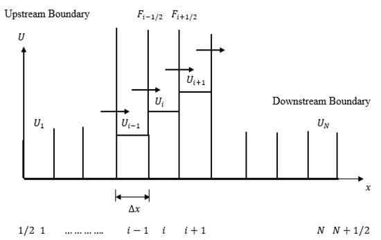
Figure 1.
Discretization used in the Finite Volume Approach [38].
Thus, the mass and momentum fluxes calculated at for all internal nodes and are as follows:
where is the average value of to the left of interface at and is the average value of u to the right of interface at . A polynomial reconstruction approach is used to estimate and whose order defines the accuracy of the numerical scheme. In Godunov’s first-order accuracy approach, the condition and is used. In the second-order Godunov scheme, the MUSCL-Hancock scheme is introduced [38,39,41] The MINMOD limiter is recommended to stop false oscillations, the features of which are found in Toro [41]. Figure 2 shows a flow chart of the second-order Godunov method for water hammer modelling with the MINMOD limiter; however, it can be replaced with any other limiter.
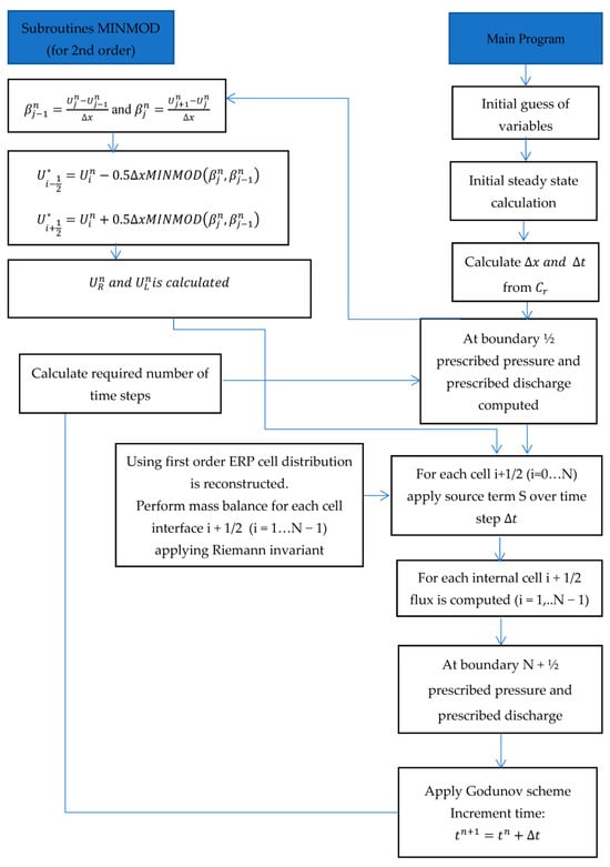
Figure 2.
Flowchart for Finite Volume Scheme using second Order Godunov approach with MINMOD limiter [29].
The following relations are obtained across each wave speed , after applying the Rankine–Hugoniot condition:
For the upstream boundary, . Similarly, for the downstream boundary, attained by combining the Riemann invariant of the equation with a pressure-flow boundary condition. Here, and where and are computed through the combination of the Riemann invariant with a pressure-flow boundary relation at time .
The unsteady friction term is added to the source term . Source terms are incorporated into the solution by time splitting utilising a second-order Runge–Kutta discretization to the following explicit methods.
First step:
Second step:
where . is updated with and has been linked to previous variables rather than .
Third step:
where . is updated with and is computed by the previous variables .
The Courant–Friedrichs–Lewy criterion is already achieved by considering that is small as compared with . Although the second-order Runge–kutta method exhibits the stability criterion as well:
Hence, the permissible time step for the source term () can be provided by the following:
Further, the maximum permissible time step with the convective term and the source term is provided by the following:
Since there is unsteady friction in the source term , the water hammer simulations may have a little stability, when . Hence the proposed stability criterion is
3. Quasi-2-D Eddy Viscosity Model
During unsteady flow conditions, wall friction affects both the magnitude and shape of pressure waves in the pipes. The fluid flow parameters, like the velocity profile, wall shear stress, and energy dissipation rate, are affected by pipe roughness during transient flow. The accurate prediction of transient waves is required for the design of water pipelines, natural gas pipelines, and pressurized sewage pipeline systems. Pezzinga [42] was the first to present a quasi-2-D turbulence model on hydraulically rough pipes. However, the quasi-2-D model [14,15,42] is computationally intensive and has only been used for simple pipe systems and boundary conditions. The model was developed by Silva-Araya and Chaudhry [14] to model unsteady friction during a slow valve closure. The model computes velocity iteratively and the convergence of iterative velocity profiles is subjected to satisfying the continuity equation. The actual friction factor product of the energy dissipation factor and steady-state friction factor at any instant was used in the method of characteristics equations to compute flow variables in the time and space domain. Hanmaiahgari and Maji [43] implemented the model developed by Silva-Araya and Chaudhry [14] to simulate sudden valve closure experiments [21] conducted at different Reynolds numbers. In this model [42,43], a quasi-steady approximation is proposed to compute the frictional losses in unsteady pipe flow. Though this method accurately predicts maximum or minimum pressure without a two-phase flow, it cannot predict the time history of the pressure profile. The quasi-steady approximation underestimates pressure damping as compared with the real system. Hence, the eddy viscosity model is used in the simulation of transient pipe flows [43]. The general governing equation for the conservation of mass and momentum [31] is expressed in the following form:
where the energy dissipation factor
The total shear stress is given as follows:
where is the shear stress due to viscosity, is the average velocity, and is the Reynolds shear stress. The Reynolds shear stress is estimated from Prandtl’s mixing length concept as follows:
The Reynolds shear stress is also estimated using the eddy viscosity principle proposed by Boussinesq
Both the eddy viscosity and mixing length models match well. The inner region uses the mixing length model and the outer region uses the eddy viscosity model. The distribution of the eddy viscosity is shown in Figure 3. The computation of the mixing length distribution is necessary for the computation of the eddy viscosity. The equation showing the relation between eddy viscosity and mixing length [44] is given as follows:
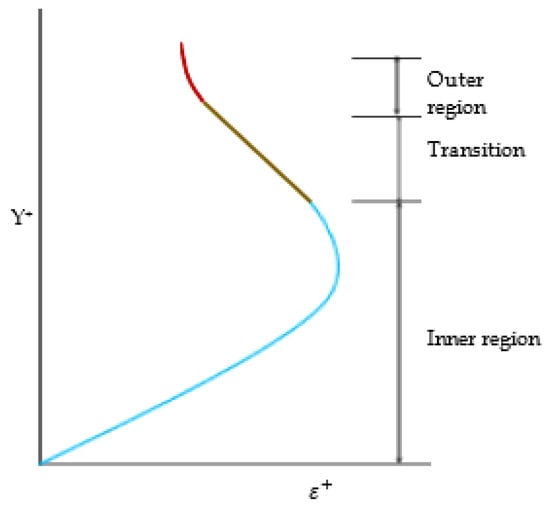
Figure 3.
Eddy viscosity distribution [43].
The mixing length equation [44,45] is given as follows:
where is mixing length damping factor for flows with zero pressure gradient [45]
The more details about the quasi 2D eddy viscosity model is found in Silva-Araya and Chaudhry [14]. Hanmaiahgari and Maji [43] evaluated the performance of the eddy viscosity model during sudden valve closure and validated it with the experimental measurements of Adamkowski and Lewandowski [21]. They compared the pressure profiles at the downstream end of pipelines for the initial flow velocity m/s and compared these with the experimental data, as shown in Figure 4. The dimensionless pressure and dimensionless time were represented by and respectively.
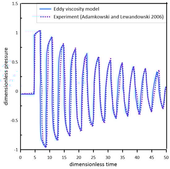
Figure 4.
Measured and computed pressure profile for sudden valve closure with initial velocity m/s [43].
The eddy viscosity model is advantageous as it computes 2D velocity profiles during unsteady flow. The limitation of the eddy viscosity model is that they are computationally intensive and need more computational time compared with convolution-based and instantenous acceleration-based methods [43]. They can be used in extended simulations for accurately locating leakages in water distribution systems.
4. Three-Dimensional CFD Modelling
4.1. Governing Equations for 3-D CFD Model
The mass and momentum equations for the 3-D CFD water hammer model are the Reynolds-Averaged Navier–Stokes equations represented in tensor notation as follows.
where is the fluid density, and are the velocity components, is the time, is the pressure, and is the fluid dynamic viscosity. For turbulent flows, the Reynolds stress tensor is modelled using a turbulence model, but it disappears for laminar flows. It is not required to solve the energy equation during the water hammer calculations since the variation in temperature is insignificant [34,46,47]. The compressibility effect is taken into consideration during the simulation, and the relationship is expressed as
where is the fluid bulk modulus, is water density, and is absolute pressure.
However, this relationship ignores the influence of pipe elasticity, which results in overestimating the wave speed and generating a higher pressure rise than the experimental data. To overcome this issue, the bulk modulus is replaced by [48]
where is the adjusted bulk modulus; is the pipe inner diameter; is the Young modulus of elastic pipe; and is the pipe wall thickness. The above correction now considers both the fluid’s compressibility and the pipe’s elasticity. Hence the wave velocity decreases as
4.2. Mesh Analysis
Results from 3-D CFD simulations are less accurate and less efficient when the mesh quality is poor. Several mesh-independent analyses with different accuracy standards were conducted in previous studies to determine the most suitable mesh size. The viscous sublayer must also be carefully selected to examine the impact of wall shear stress on other variables. Most of the studies considered the three mesh parameters, as suggested by Martins et al. [49], were measured in the axial direction measured in the tangential direction and = FLT/, the ratio of first layer thickness (FLT) to the thickness of the turbulent flow viscous sublayer determined in the radial direction, beginning near the wall and advancing in a core direction. The distribution of grid nodes is concentrated in the proximity to the pipe wall, as shown in Figure 5.
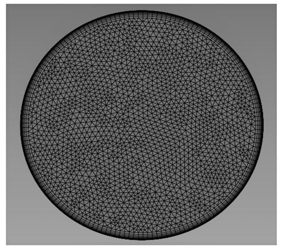
Figure 5.
Three-dimensional mesh in pipe cross-section [46].
Cao et al. [50] conducted a greater number of meshing techniques to analyse the effects of grid density on 3-D CFD simulation results. It was found that both the numerical accuracy and computing cost rise with higher grid densities. The 3-D simulations can achieve high precision and cost-effective computation at some suggested value of grid densities. Higher grid density does not improve accuracy when it exceeds the recommended values; instead, it increases calculations and leads to numerical instability.
4.3. Turbulence Modelling
Solving the RANS equation directly can lead to a closure problem because the Reynolds stresses are non-linear and unknown [51]. Turbulence models are employed to provide the mathematical closure to equations of motion. They are defined as semi-empirical formulations of Reynolds stresses in terms of average velocity gradients. Ghidaoui et al. [2] presented an interesting nondimensional parameter defined as the ratio of the time scale of the delay in turbulence production to the time scale of the pressure wave. It is given as follows:
where is the inside diameter of the pipe, is the pipe length, is friction velocity dependent on the Darcy–Weisbach friction factor and the mean steady-state velocity, and is the speed of the wave. Based on the magnitude of the parameter , three regimes were observed by Ghidaoui et al. [2]. When , the steady-state flow’s structure and intensity of turbulence are identical to those of transient flow. This indicates that in these types of flows, the steady-state turbulence model remains valid. When , variations in the structure and intensity of turbulence during water hammer can be seen. There is sufficient time for the turbulence to propagate towards the centre of the pipe, thereby the viability of the steady-state turbulence models should be examined. When , the consequences of the water hammer are negligible.
Of all the turbulence models that the ANSYS FLUENT 2022 R2 (22.2) offers, the - model utilizes less computational resources in modelling flows and is most preferred in engineering applications [13,47,52]. The mathematical formulation of the (Re-Normalization Group) RNG - has a similarity with the standard - but with some modifications [53,54]. The RNG-based - turbulence model is generated from the instantaneous Navier–Stokes equations utilising a mathematical method called “renormalization group” (RNG) methods. The eddy viscosity approximation is used in the RNG k- turbulence model to calculate the Reynolds stress tensor in the momentum equation. Saemi et al. [55] carried out 2-D axisymmetric calculations based on unsteady Reynolds-averaged Navier–Stokes (URANS) equations and a high Reynolds RNG - model. They found that the high Reynolds RNG - model cannot reproduce more accurate wall shear stress distributions and other characteristics of turbulent water hammers close to the wall.
The realizable - model fulfils certain mathematical limitations on the Reynolds stresses that are consistent with turbulent flow physics. The Boussinesq hypothesis is used to establish the relationship between the Reynolds stresses and the mean velocity gradients in the model. The Boussinesq hypothesis is preferred over the Reynolds stress model (RSM) because of the low computational cost involved in the calculation of turbulent viscosity. Previous works on separated flows and flows with complex secondary flow characteristics have demonstrated that the realizable model yields good results compared with all other - models.
where is the turbulent kinetic energy, is the kinetic eddy viscosity, and is mean velocity gradient, defined as
The extra transport equations ( and ) specific for the realizable - model are expressed as follows:
where is the turbulence kinetic energy generation due to the mean strain rate; is the contribution of the fluctuating dilatation in compressible turbulence to the overall dissipation rate; is the generation of turbulence kinetic energy due to buoyancy; and are the turbulent Prandtl numbers for and , respectively; is the turbulent viscosity; max; ; ; and and are constants. Yang et al. [1], Martins et al. [13,56], Wu et al. [57], and Ferreira et al. [58] employed the realizable - model in the 3-D CFD model for the simulation of water hammer problems. The realizable - model has the drawback of producing non-physical turbulent viscosities in case of multiple reference frames and rotating sliding meshes where the computational domain contains rotating and stationary fluid zones The other drawback of the - model is that it needs to be modified to be appropriate for unsteady turbulent flows with adverse and favourable pressure gradients [59].
A more accurate prediction of the transient pressure during valve closure can be possible with the shear stress transport - model [50,60]. The refined mesh and the contribution of the boundary layer both have a considerable impact on the correct estimation of shear stress, which is easily incorporated into the SST - model. The Boussinesq approximation is used in - model to derive the unknown Reynolds stress tensor as
where is the specific rate of dissipation, is the kinematic eddy viscosity, and is the Kronecker delta.
The extra transport equations ( and ) specific for the SST - model are expressed as follows:
where is the turbulence kinetic energy generation due to the mean strain rate; and are the dissipation of and due to turbulence; is the generation of ; and are the effective diffusivity of and , respectively; represents the cross-diffusion term; and and are source terms. Saemi et al. [55] simulated 2-D axisymmetric calculations for laminar as well as turbulent water hammer flows using unsteady Reynolds-averaged Navier–Stokes equations. They employed the low Reynolds SST - model and high Reynolds RNG - model and found that the low Reynolds SST - model can produce better pressure variations that match with experimental results. Kalantar et al. [61] and Saemi et al. [62] applied the SST - model for the 3-D simulation of water hammer problems.
4.4. Various 3-D CFD Approaches in Water Hammer Modelling
CFD solvers are set up with suitable boundary conditions which define the physics of fluid flow. At the inlet boundary, a constant pressure is set and at the outlet boundary, a time domain mass outflow is given, as shown in Figure 6. Three different cases of valve closure: instantaneous, linear, and flow rate reduction curves obtained from 3D valve modelling are also presented in Figure 7.
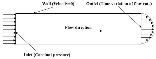
Figure 6.
Boundary conditions for 3-D simulation [47].
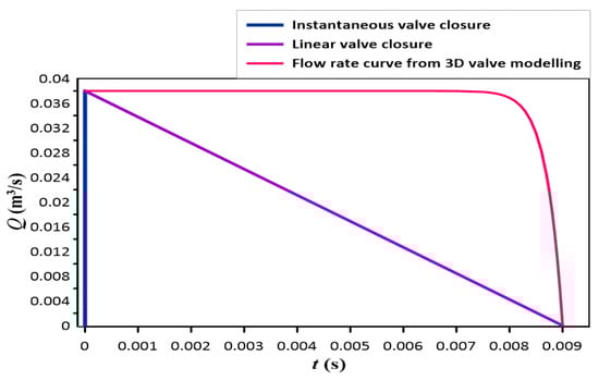
Figure 7.
Flow rate curve for three different scenarios [46].
The flow velocity is reduced linearly from a steady state to zero at the outlet to represent the valve closure in the simulation of laminar water hammer flow by Karney et al. [63]. There was a good agreement in pressure variations between the experimental data and CFD results as compared with MOC models. Martins et al. [47] simulated water hammer flow using a 3-D URANS and k- turbulence model. The study utilised a three-dimensional effective mesh created by Martins et al. [49] and the discharge reduction curve as the outlet boundary condition as defined by Wylie and Streeter [64]. The discharge reduction curve only enhanced the slope of the pressure change and no variation was found between the results of 3-D water hammer predictions and 2-D axisymmetric computations utilising such a simple boundary condition. Saemi et al. [46] investigated 2-D axisymmetric simulations for water hammer flow in FLUENT where a discharge reduction curve was used as an outlet boundary condition. The study showed that using the discharge curve generated from 3-D simulations increases the accuracy of 2-D axisymmetric calculations resulting in identical prediction in 2-D and 3-D. In the present work, the results of the 3-D CFD simulation using the flow rate curve as an outlet boundary condition are validated with the experimental data of Bergant et al. [34]. The pipe system was made of 37.2 m long copper pipe, with 0.022 m diameter and 1.6 mm wall thickness. The initial steady-state flow rate was taken to be 0.076 × 10⁻⁵ m3/s and the upstream reservoir head as 32 m. A downstream ball valve was closed rapidly in 0.009 s. Figure 8a,b shows the excellent match of the 3-D CFD pressure history at the valve and midpoint of the pipe with its experimental counterpart.
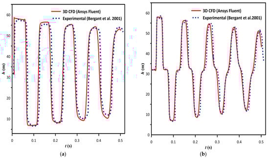
Figure 8.
Comparison of pressure head () variation with time ( between CFD simulations and experimental data [34]: (a) at valve (b) at the midpoint of the copper pipeline.
The 3-D valve modelling method is incapable of visualizing the 3-D flow structures generated by the valve closure inside the domain. Advanced valve modelling techniques are necessary to obtain accurate results. Hence, several studies focused on modelling valve closure based on the dynamic mesh technique. Dynamic mesh is often used in simulations of rotating equipment, oscillating structures, fluid-structure interactions, and free-surface flows with changing fluid domains due to motion on domain boundaries. ANSYS FLUENT 2022 R2 (22.2) let users specify domain motion with boundary profiles or user-defined functions. The geometry consists of two domains: Domain 1 represents the portion of pipe upstream and downstream to the valve and Domain 2 represents the valve’s space in the pipe. The lower region of the valve is represented by the upper region of domain 2. As the valve moves into the pipe represented by the downward moving arrow in Figure 9, the volume of domain 2 starts reducing. The valve (solid) part is seen between domains 1 and 2 as it moves inside the pipe. Interfaces connecting the domains are updated at every time step.
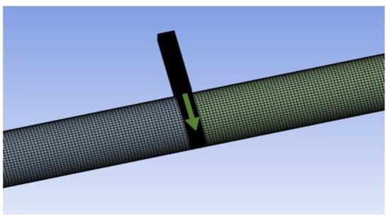
Figure 9.
Part of the pipe geometry shows the gate valve moving inside the pipe [65].
ANSYS FLUENT 2022 R2 (22.2) is used in this study since it allows both smoothing and re-meshing at every time step. Neyestanaki et al. [65] employed the spring/Laplacian-based smoothing method. This method brings each mesh vertex closer to the geometric centre of its surrounding vertex. Using smoothing for larger displacement causes cell deformation to become greatly skewed. As a result, re-meshing with triangular or tetrahedral mesh is employed when the mesh is more sensitive to mesh changes [65].
Saemi et al. [62,66,67] employed a dynamic mesh approach for modelling axial gate valve closure. The static pressure at the outlet and the total pressure at the inlet are used in the simulation. The limitation of the dynamic mesh technique is that re-meshing is time-consuming and can result in divergence near the end of the closure of the valve when re-meshing is carried out in a smaller region [61]. In summary, dynamic mesh is a powerful technique that enables fluid dynamics in complicated systems to be simulated with realistic and greater precision.
The sliding mesh approach provides accurate results when transient interaction between fixed and rotating components is desired in the flow simulations. More than one cell zones are utilised in the sliding mesh approach; the mesh is created locally in each zone. Each zone (stationary or moving) is surrounded by one or more “interface zones” that connect to the neighbouring cell zone. The two cell zones move relative to one another along the mesh interface during the calculation. The sliding mesh technique is utilised for modelling the dynamic course of the ball valve closing as shown in Figure 10. The valve body rotates around its centre during the closing operation and the two pairs of spherical surfaces act as interface surfaces. The area of contact between the two interfaces is reduced as the valve body starts rotating, and after a certain angle, the interface surfaces are completely separated. Due to the loss of contact between the interfaces at their intersection, no fluid can move between these two regions, which denotes complete valve closure.
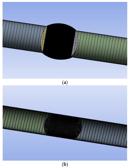
Figure 10.
Ball valve geometry in (a) 100% valve closure, (b) complete valve open [46].
Yang et al. [1] used a 3-D computational fluid dynamics model with the sliding mesh method for modelling water hammer and compared those results with 1-D MOC calculations based on unsteady friction models. The results also demonstrated that sliding mesh is a reliable technique for simulating the rapid closing of rotating ball valves. Saemi et al. [46] investigated 3-D numerical simulation for laminar and turbulent water hammer flow which utilized a sliding mesh approach for closing the valve. In this study, the axisymmetric model was also used in which the flow rate reduction was used as an outlet boundary condition. However, compared with the axisymmetric simulations, 3-D CFD simulations using sliding mesh provided accurate pressure variation results; however, they required vast computational resources. The sliding mesh technique was utilized to realize the rotation process of the ball valve to analyse the impact of various closing laws and closing times on the water hammer [68]. Cao et al. [50] developed a 3-D CFD model to study the 3-D dynamic features of the ball valve closure. The ball valve closure was accomplished by utilising the sliding mesh technique. It was observed that during the closing operation, mean velocity variations and differential pressure at the valve underwent three different stages. The axial motion of a thin gate valve can be modelled as a mesh movement without any deformation using the sliding mesh technique [65]. This approach predicts more accurate outcomes that are closer to the experimental measurements. The sliding mesh is the most preferred approach for valve closure modelling in the literature as they are less expensive and present more accurate results.
In this approach, the domain used to model the valve body is known as an immersed solid domain. The solid domain is immersed into the fluid region represented by the pipe indicating the valve closure process shown clearly in Figure 11b. In the overlapping of solid and fluid regions, the immersed solid technique introduces a source term in the momentum equation to force the fluid velocity to match the velocity of the immersed solid. Kalantar et al. [61] employed the immersed solid method for modelling the valve closure to study the pressure-time method during the water hammer phenomenon. The study showed that there could be a chance for the leaking of water through the immersed solid as the valve starts closing. Neyestanaki et al. [65] presented and compared various methods for axial valve closure in a 3-D water hammer simulation. The result showed that the immersed solid approach underestimates differential pressure rise and overestimates wall shear stress close to the end of valve closing due to a lag in discharge reduction. In the case of axial valve motion, the immersed solid approach is easier and preferable to the dynamic mesh approach because the need for mesh deformation and re-meshing is eliminated in the method [65,69].
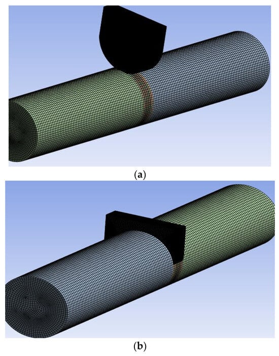
Figure 11.
(a) fluid domain and immersed solid domain at , (b) overlapping of the fluid domain and immersed solid domain at the time for modelling valve closure [65].
5. Turbulence Structures in Accelerating and Decelerating Flows
The accelerating turbulent pipe flow occurs when there is a sudden valve opening, a step increase in flow rate, a pump starting, and load acceptance in turbines. A turbulent flow in a pipe suddenly accelerates subjected to a total acceleration greater than zero, as in Equation (47) where is the average velocity of the flow.
The decelerating turbulent pipe flow occurs when there is a sudden valve closing, a step decrease in flow rate, a pump tripping, and load rejection in turbines. A steady flow in a pipe is suddenly decelerated if total acceleration is less than zero.
Figure 12 and Figure 13 show the velocity profile in the case of accelerating and decelerating flows, respectively.
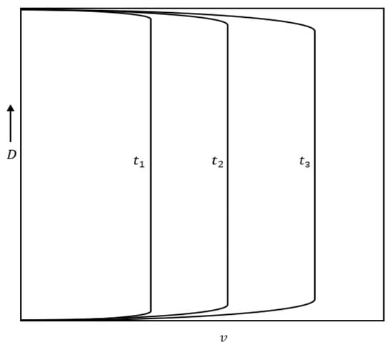
Figure 12.
Typical velocity profile in an accelerating pipe flow (.
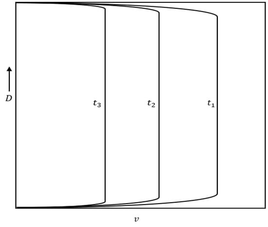
Figure 13.
Typical velocity profile in a decelerating pipe flow.
Most fluid conveyance methods through pipes are not steady from the industrial perspective. In addition, control valves or pumps continuously adjust the flow through pipes to satisfy certain demands. Most engineering designs exclude transient effects in unsteady flows because of a lack of understanding about such flows. Hence, to estimate the frictional drag in accelerating, as well as decelerating, pipe flow, not many valid unstable friction models are available. Uncertainty regarding the transitional mechanisms and durations of the various transitional stages may result from the chosen step-down size or the masking impact caused by the flow structures at the start of the transient. The study of turbulence structures in accelerated and decelerated flows is important to an in-depth understanding of unsteady friction.
The comparison between sudden accelerated flows and sudden decelerated flows indicates that the velocity profile is more stable in an accelerating flow than in that of a decelerating flow [70,71]. Therefore, there may be a significant variation in how accelerating and decelerating flows behave. Vardy and Brown [71] investigated a specific type of unsteady flow where a steady flow through the pipe is abruptly accelerated. The general flow pattern and the presence of the radially travelling viscosity front, in particular, are the properties of suddenly accelerating flows. The accelerated flow is defined by three different stages. There is a lag in the turbulence response at stage 1, then a strong turbulence response at stage 2, and in stage 3 there exists a persistent lag in the response that resembles a succession of quasi-steady states. Turbulence’s axial components show a sudden response, while the corresponding changes in radial and tangential components occur much later. The effects of varying the pipe diameter, the initial Reynolds number, and the acceleration rate on the flow characteristics were investigated by He et al. [70]. Their study showed that the most essential pattern of behaviour during stage 1 remained the same across all the cases, despite major variations existing in stages 2 and 3. The turbulence models utilized in the analysis of accelerated and decelerated flows by Vardy and Brown [71] predicted similar qualitative behaviour, but there were major variations in when and how the delayed turbulence response to the acceleration triggers the radially moving front. The effect of a water-hammer wavefront is identical to a sudden shift in axial velocity at a given axial location, and then a slow shift in the radial velocity distribution [71]. The two common characteristics regarding the prescribed turbulent viscosity distributions are that they approximate the radial distributions of the effective viscosity and with regard to the selected distributions as frozen. They concluded that only the first of the three flow stages can be approximated by assuming unaffected effective viscosity from the previous steady flow. This stage’s predictions are slightly insensitive to the turbulence model; therefore, they can be used to support simplified models.
The behaviour of the mean wall shear stress and its sporadic nature directly affect the energy cost of transportation networks. Using the direct numerical simulation data sets of turbulent flow in a pipe at various Reynolds numbers, Guerrero et al. [72] investigated the highly intermittent nature of wall shear stress and its relation with other flow parameters. The analysis provided a thorough understanding of the flow dynamics responsible for backflow events, their connection to the larger scales of motion in the outer region, and their impact on turbulence production, turbulent inertia, and viscous dissipation. They demonstrated that the presence of two large-scale anticlockwise rotating motions in the buffer zone plays a crucial role in the prevalence of backflow events. Extremely positive streamwise wall shear stress regions are produced by an intense quasi-streamwise vortex which carries streamwise momentum from overlap and outer regions towards the wall.
5.1. Accelerating Flows
Guerrero et al. [73] investigated the characteristics of accelerating turbulent pipe flows after a quick increase in flow rate from a more detailed perspective. A high-spatiotemporal DNS data set was employed for this purpose. Maruyama et al. [74] described a delayed response in turbulence in the seminal investigation of a step-wise accelerating turbulent flow through pipes linked to two lags one with new turbulence and the second with the wall-normal diffusion of vorticity caused by the acceleration exerted on an already turbulent base flow. Further, He and Jackson [75] observed a third lag due to the redistribution of TKE among the three orthogonal velocity components. Greenblatt and Moss [76], using single-component LDV, collected time series data sets of quickly accelerating pipe flow. The result revealed that displacement thickness, as well as momentum thickness, showed coherence with the progression of time. Jung and Hung [77] used large eddy simulation data sets to replicate the investigations of He and Jackson [75]. These simulation results also supported the three-phase lags in the turbulence response. Using DNS, Guerrero et al. [73] examined the phases that occur in turbulent flow as the flow rate is rapidly increased, as measured by the temporal evolution of dynamic variables in the mean momentum balance. Inertial, pre-transition, transition, and core relaxation are the four distinct phases that characterise the transient behaviour of a turbulent flow after a rapid temporal acceleration [76,78]. According to the results, an equilibrium in the skin friction coefficient is not always a reliable predictor of when the flow is to reach its final steady state. By analysing the transient nature of the largest uniform momentum zone of the flow, and the core region during the last transitional phase, this study explains the delayed regeneration of turbulence in the flow’s wake zone utilizing the methods proposed by Guala et al. [79]. These findings pave the way for the creation of more accurate unsteady friction models and provide a deeper insight into the dynamics of unsteady turbulent pipe flow [27,71,80]. The temporal evolution of turbulent eddies, flow dynamics, momentum distribution, and Reynolds and viscous shear stresses is analyzed to determine the relationship between flow dynamics and frictional drag, particularly at inertial and core-relaxation periods [73]. Figure 14a shows a linear increment in the Bulk Reynolds number () on a time domain scaled by the initial viscous units () and Figure 14b depicts the time response of the skin friction coefficient () [73].
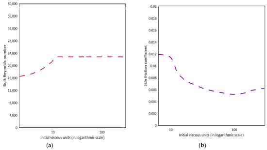
Figure 14.
(a) Time evolution of the bulk Reynolds number () on a time domain scaled by the initial viscous units (), (b) Transient response of skin friction coefficient () [73].
Over the past ten years, there has been an emphasis on the temporal response of frictional drag in accelerating turbulent pipe and channel flows [81]. Several numerical analyses have been conducted in this area [78,82]. Using DNS data sets, He and Seddighi [78] investigated the time dependency of the mean skin friction coefficient as well as other mean flow statistics to identify the phases encountered by a turbulent channel flow after a quick increase in discharge. According to the findings, in a suddenly accelerated turbulent channel flow resembles the bypass transition of a turbulent boundary layer. Also, a suddenly accelerated channel flow goes through two transient phases: pretransition and transition. During the pretransition phase, a perturbation boundary layer forms as a result of a plug-like inflow into the turbulent base flow, whose turbulence remains fixed at first. Hence the skin friction coefficient declines, reaching its lowest value at a point where the pre-transitional phase ends and the transitional phase starts. The skin friction coefficient returns to its original value during the transition phase as a result of the formation of ‘new’ turbulent areas that expand, merge, and spread across the whole flow domain. The skin friction coefficient reaches an equilibrium as the flow is fully developed. Guerrero et al. [73] utilized DNS data sets to analyze the transient flow dynamics of a series of suddenly accelerated turbulent pipe flows between two steady Reynolds numbers (Re). The temporal variation in the mean flow dynamics showed coherence and demonstrated that a suddenly accelerated internal flow goes through four transient phases, namely inertial (phase I), defined by viscous forces that grow rapidly and a turbulent behaviour freezes; pre-transition (phase II), a quick decay of viscous forces and a slow turbulence response near the wall; transition (phase III), viscous and turbulent forces rising proportionally in the inner region; and core relaxation (phase IV), turbulence moving slowly from the wall to the wake zone.
5.2. Decelerating Flows
The decelerating flows show ‘frozen’ turbulence behaviour similar to accelerating flows in the early flow excursion [74,81]. Maruyama et al. [74] carried out a similar experimental investigation that shows that the total kinetic energy decays at a roughly linear rate following the initial “frozen turbulence” period. By analyzing the time series of the average frictional velocity and the average centerline velocity , a decelerating flow is followed by two transient phases that have rapid and slow time responses [83]. However, it does not explain the mechanisms underlying these two distinct relaxation times. More recently, the total kinetic energy production budget has been divided into three parts and their behaviour is analyzed for accelerating and decelerating flows by Joel and Sundstrom [84]. They concluded that the turbulence establishment in those two unsteady flows varies significantly. Only a limited number of studies are available on the time variation in the mean skin friction coefficient and the near-wall dynamics related to the time-varying decelerating internal flow, and the majority of them do not examine frictional drag throughout the entire transient phase [81,85]. There have been very few attempts to analyze the transient frictional drag in decelerated internal flows using DNS [82,83].
Guerrero et al. [86] investigated the turbulence flow dynamics and time response experienced by sudden decelerating turbulent flow through pipes using direct numerical simulation data sets of linearly decelerated turbulent pipe flows. The turbulence response of a fully developed turbulent flow exhibits a phase lag when the flow is subjected to linear acceleration. It is concluded from the study that (i) there is a phase lag in the turbulence response of a quickly decelerating flow, as is shown in studies of accelerating flows as well; (ii) the presence of large-scale layers of negative azimuthal vorticity near the wall is indicated by the fact that the viscous stress can become negative there; (iii) when a flow excursion occurs, the viscous force’s sign switches in the viscous sublayer from negative to positive, and this change propagates in the direction normal to the wall by viscous diffusion; and (iv) the shape of the average velocity profile is changed within the near-wall zone and its linear behaviour is recovered during this time. However, the overlap and wake regions of the flow do not change, which indicates that the outer flow turbulence freezes. (v) Meanwhile, the near-wall region displays a stationary mean velocity profile. Figure 15a shows a ramp down in flow rate was enforced at to rapidly reduce the Reynolds number and Figure 15b depicts that the time response of the skin friction coefficient indicates that flow undergoes several transient behaviours before becoming stationary [86].
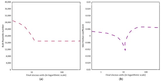
Figure 15.
(a) Ramp-down change of the bulk Reynolds number () on a time domain scaled by the Final viscous units (), (b) Transient response of the skin friction coefficient () [86].
6. Future Research Directions
Parallel computing techniques are receiving attention as they reduce computational time and costs. Parallel computing has been increasingly accessible, affordable, and widely applied as the number of available supercomputers has grown. Graphical processing units (GPUs) offer appealing features for large-scale computing [87]. Parallel computing with the GPUs together can improve the computational resources required for 3-D CFD studies.
Advancing our understanding of fluid–structure interaction may be possible with the use of 2D and 3D finite volume modelling that can capture turbulence-driven vortices in transient flow It can help in analyzing problems like pipe incrustation, and wall erosion enabling preventive and rehabilitation actions. Hence, the developments in numerically precise models can help in cost savings and prevent issues in pipe design, management, and operational domains.
7. Conclusions
Designing, operating, and assessing the risks associated with a pipeline system require transient analysis. This article provides historical developments of water hammer modelling, focussing particularly on the recent CFD simulation in improving the transient flow numerical prediction. This study briefly reviewed the application of Godunov’s second-order finite volume method (FVM) technique in solving water hammer equations with unsteady friction and the discussion is extended to the application of the quasi-2-D eddy viscosity turbulence closure model. This paper reviewed the pros and cons of the sliding mesh, immersed solid approach, and the dynamic mesh approaches for modelling valve closures. Based on findings from previous literature, this study concludes that the sliding mesh approach is less expensive than other methods and is utilised mostly for valve closure modelling. However, the valve modelling techniques require vast computational resources. This study shows the 3-D CFD simulation with a flow rate reduction curve as a boundary condition accurately predicts the pressure variation close to the experimental results. Finally, a brief overview of the transient flow turbulence structures for a rapidly accelerated and decelerated pipe flow using DNS (direct numerical simulation) data sets is presented. Overall, this paper summarised past developments and future scope in the field of water hammer modelling using CFD.
Author Contributions
M.R.A.K.: writing and original draft preparation; P.R.H.: writing—review and editing, project administration, and funding acquisition; J.H.P.: writing—review and editing and funding acquisition; M.F.L.: writing—review and editing and funding acquisition. All authors have read and agreed to the published version of the manuscript.
Funding
This research received no external funding.
Data Availability Statement
The data presented in this study are available on request from the corresponding author.
Conflicts of Interest
The authors declare no conflict of interest.
References
- Yang, S.; Wu, D.; Lai, Z.; Du, T. Three-Dimensional Computational Fluid Dynamics Simulation of Valve-Induced Water Hammer. J. Mech. Eng. Sci. 2017, 231, 2263–2274. [Google Scholar] [CrossRef]
- Ghidaoui, M.S.; Asce, M.; Sameh; Mansour, G.S.; Zhao, M. Applicability of Quasisteady and Axisymmetric Turbulence Models in Water Hammer. J. Hydraul. Eng. 2002, 128, 917–924. [Google Scholar] [CrossRef]
- Lohrasbi, A.R.; Attarnejad, R. Water Hammer Analysis by Characteristic Method. Am. J. Eng. Appl. Sci. 2008, 1, 287–294. [Google Scholar] [CrossRef]
- Meniconi, S.; Ferrante, M. In-Line Partially Closed Valves: How to Detect by Transient Tests. In Proceedings of the World Environment and Water Resource Congress, Kansas City, MO, USA, 17–21 May 2009; pp. 135–144. [Google Scholar]
- Pal, S.; Hanmaiahgari, P.R.; Karney, B.W. An Overview of the Numerical Approaches to Water Hammer Modelling: The Ongoing Quest for Practical and Accurate Numerical Approaches. Water 2021, 13, 1597. [Google Scholar] [CrossRef]
- Pu, J.H.; Shao, S.; Huang, Y. Numerical and Experimental Turbulence Studies on Shallow Open Channel Flows. J. Hydro-Environ. Res. 2014, 8, 9–19. [Google Scholar] [CrossRef]
- Hui Pu, J.; Shao, S.; Huang, Y.; Hussain, K. Evaluations of SWEs and SPH Numerical Modelling Techniques for Dam Break Flows. Eng. Appl. Comput. Fluid Mech. 2013, 7, 544–563. [Google Scholar] [CrossRef]
- Pu, J.H.; Cheng, N.S.; Tan, S.K.; Shao, S. Source Term Treatment of SWEs Using Surface Gradient Upwind Method. J. Hydraul. Res. 2012, 50, 145–153. [Google Scholar] [CrossRef]
- Pu, J.H.; Pandey, M.; Li, J.; Satyanaga, A.; Kundu, S.; Hanmaiahgari, P.R. Editorial: The Urban Fluvial and Hydro-Environment System. Front. Environ. Sci. 2022, 10, 1075282. [Google Scholar] [CrossRef]
- Brunone, B.; Ferrante, M.; Cacciamani, M. Decay of Pressure and Energy Dissipation in Laminar Transient Flow. ASME J. Fluids Eng. 2004, 126, 928–934. [Google Scholar] [CrossRef]
- Riasi, A.; Nourbakhsh, A.; Raisee, M. Energy Dissipation in Unsteady Turbulent Pipe Flows Caused by Water Hammer. Comput. Fluids 2013, 73, 124–133. [Google Scholar] [CrossRef]
- Meniconi, S.; Brunone, B.; Ferrante, M.; Massari, C. Energy Dissipation and Pressure Decay during Transients in Viscoelastic Pipes with an In-Line Valve. J. Fluids Struct. 2014, 45, 235–249. [Google Scholar] [CrossRef]
- Martins, N.M.C.; Brunone, B.; Meniconi, S.; Ramos, H.M.; Covas, D.I.C. CFD and 1D Approaches for the Unsteady Friction Analysis of Low Reynolds Number Turbulent Flows. J. Hydraul. Eng. 2017, 143, 04017050. [Google Scholar] [CrossRef]
- Silva-Araya, W.F.; Chaudhry, M.H. Computation of Energy Dissipation in Transient Flow. J. Hydraul. Eng. 1997, 123, 108–115. [Google Scholar] [CrossRef]
- Reddy, H.P.; Asce, M.; Walter; Silva-Araya, F.; Chaudhry, M.H.; Asce, F. Estimation of Decay Coefficients for Unsteady Friction for Instantaneous, Acceleration-Based Models. J. Hydraul. Eng. 2012, 138, 260–271. [Google Scholar] [CrossRef]
- Wang, L.Q.; Li, Z.F.; Wu, D.Z.; Hao, Z.R. Transient Flow around an Impulsively Started Cylinder Using a Dynamic Mesh Method. Int. J. Comut Fluid. Dyn. 2007, 21, 127–135. [Google Scholar] [CrossRef]
- Godunov, S.K. A Difference Method for the Numerical Calculation of Discontinuous Solutions of Hydrodynamic Equations. Mat. Sb. 1959, 89, 271–306. [Google Scholar]
- Pal, S.; Kottam, R.R.; Lambert, M.F.; Hanmaiahgari, P.R. Estimation of Deposit Thickness in Single-Phase Liquid Flow Pipeline Using Finite Volume Modelling. J. Pipeline Sci. Eng. 2023, in press. [Google Scholar] [CrossRef]
- Pu, J.H. Turbulence Modelling of Shallow Water Flows Using Kolmogorov Approach. Comput. Fluids 2015, 115, 66–74. [Google Scholar] [CrossRef]
- Wylie, E.B.; Streeter, V.L.; Suo, L. Fluid Transients in Systems; Prentice Hall: Englewood Cliffs, Bergen, NJ, USA, 1993. [Google Scholar]
- Adamkowski, A.; Lewandowski, M. Experimental Examination of Unsteady Friction Models for Transient Pipe Flow Simulation. ASME J. Fluids Eng. 2006, 128, 1351–1363. [Google Scholar] [CrossRef]
- Zielke, W. Frequency-Dependent Friction in Transient Pipe Flow. J. Basic. Eng. Trans. ASME 1968, 90, 109–115. [Google Scholar] [CrossRef]
- Trikha, A.K. An Efficient Method for Simulating Frequency Dependent Friction in Transient Liquid Flow. ASME J. Fluids Eng. 1975, 97, 97–105. [Google Scholar] [CrossRef]
- Kagawa, T. High Speed and Accurate Computing Method of Frequency-Dependent Friction in Laminar Pipe Flow for Characteristic Method. JSME Int. J. Ser. B 1983, 49, 2638–2644. [Google Scholar] [CrossRef]
- Suzuki; Takayuki Taketomi, K.; Sato, S. Improving Zielke’s Method of Simulating Frequency-Dependent Friction in Laminar Liquid Pipe Flow. ASME J. Fluids Eng. 1991, 113, 569–573. [Google Scholar] [CrossRef]
- Vardy, A.E.; Brown, J.M.B. Transient, Turbulent, Smooth Pipe. J. Hydraul. Res. 1995, 33, 435–456. [Google Scholar] [CrossRef]
- Vardy, A.E.; Brown, J.M.B. Transient Turbulent Friction in Smooth Pipe Flows. J. Sound Vib. 2003, 259, 1011–1036. [Google Scholar] [CrossRef]
- Vardy, A.E.; Brown, J.M.B. Transient Turbulent Friction in Fully Rough Pipe Flows. J. Sound. Vib. 2004, 270, 233–257. [Google Scholar] [CrossRef]
- Pal, S.; Hanmaiahgari, P.R.; Lambert, M.F. Efficient Approach toward the Application of the Godunov Method to Hydraulic Transients. J. Hydroinformatics 2020, 22, 1370–1390. [Google Scholar] [CrossRef]
- Vítkovský, J.P.; Bergant, A.; Simpson, A.R.; Asce, M.; Lambert, M.F. Systematic Evaluation of One-Dimensional Unsteady Friction Models in Simple Pipelines. J. Hydraul. Eng. 2006, 132, 696–708. [Google Scholar] [CrossRef]
- Chaudhry, M.H. Applied Hydraulic Transients; Springer: New York, NY, USA, 2014. [Google Scholar]
- Carstens, M.R.; Rollers, J.E. Boundary-Shear Stress in Unsteady Turbulent Pipe Flow. J. Hydraul. Div. 1959, 85, 67–81. [Google Scholar] [CrossRef]
- Brunone, B.; Golia, U.M.; Greco, M. Some Remarks on the Momentum Equation for Fast Transients. In Proceedings of the International Meeting on Hydraulic Transients with Water Column Separation (9th Round Table of the IAHR Group), Valencia, Spain, 4–6 September 1991; pp. 201–209. [Google Scholar]
- Bergant, A.; Simpson, A.R.; Vítkovský, J. Developments in Unsteady Pipe Flow Friction Modelling. J. Hydraul. Res. 2001, 39, 249–257. [Google Scholar] [CrossRef]
- Ramos, H.; Covas, D.; Borga, A.; Loureiro, D. Surge Damping Analysis in Pipe Systems: Modelling and Experiments. J. Hydraul. Res. 2004, 42, 413–425. [Google Scholar] [CrossRef]
- Vítkovský, J.P.; Lambert, M.F.; Simpson, A.R.; Bergant, A. Advances in Unsteady Friction Modelling in Transient Pipe Flow. In Proceedings of the 8th International Conference on Pressure Surges, The Hague, The Netherlands, 12–14 April 2000. Water Distribution Networks Optimization View Project Acoustic Methods for Leak Detection in Water Networks View Project. [Google Scholar]
- Vítkovský, J.; Stephens; Mark; Bergant, A.; Simpson, A.; Asce, M.; Lambert, M. Numerical Error in Weighting Function-Based Unsteady Friction Models for Pipe Transients. J. Hydraul. Eng. 2006, 132, 709–721. [Google Scholar] [CrossRef]
- Zhou, L.; Li, Y.; Zhao, Y.; Ou, C.; Zhao, Y. An Accurate and Efficient Scheme Involving Unsteady Friction for Transient Pipe Flow. J. Hydroinformatics 2021, 23, 879–896. [Google Scholar] [CrossRef]
- Zhou, L.; Wang, H.; Liu, D.; Ma, J.; Wang, P.; Xia, L. A Second-Order Finite Volume Method for Pipe Flow with Water Column Separation. J. Hydro-Environ. Res. 2017, 17, 47–55. [Google Scholar] [CrossRef]
- Zhao, M.; Ghidaoui, M.S.; Asce, M. Godunov-Type Solutions for Water Hammer Flows. J. Hydraul. Eng. 2004, 130, 341–348. [Google Scholar] [CrossRef]
- Toro, E.F. Riemann Solvers and Numerical Methods for Fluid Dynamics, 3rd ed.; Springer: Berlin, Germany, 2009. [Google Scholar]
- Pezzinga, G. Quasi-2D Model for Unsteady Flow in Pipe Networks. J. Hydraul. Eng. 1999, 125, 676–685. [Google Scholar] [CrossRef]
- Hanmaiahgari, P.R.; Maji, S. Eddy Viscosity Turbulence Model for Incompressible Fluid Flow in Closed Conduits. In Proceedings of the 19th IAHR-APD Congress, Hanoi, Vietnam, 21 September 2014. [Google Scholar]
- Granville, P.S. A Modified Van Driest Formula for the Mixing Length of Turbulent Boundary Layers in Pressure Gradients. ASME J. Fluid Eng. 1990, 12, 777–849. [Google Scholar] [CrossRef]
- Araya, W.F.S. Silva-Araya Energy Dissipation in Transient Flow. Ph.D. Thesis, Washington State University, Pullman, WA, USA, 1993. [Google Scholar]
- SaemI, S.; Raisee, M.; Cervantes, M.J.; Nourbakhsh, A. Computation of Two- and Three-Dimensional Water Hammer Flows. J. Hydraul. Res. 2019, 57, 386–404. [Google Scholar] [CrossRef]
- Martins, N.M.C.; Soares, A.K.; Ramos, H.M.; Covas, D.I.C. CFD Modeling of Transient Flow in Pressurized Pipes. Comput. Fluids 2016, 126, 129–140. [Google Scholar] [CrossRef]
- Korteweg, D.J. Ueber Die Fortpflanzungsgeschwindigkeit des Schalles in Elastischen Röhren; Wiely: Hoboken, NJ, USA, 1878. [Google Scholar]
- Martins, N.M.C.; Carriço, N.J.G.; Ramos, H.M.; Covas, D.I.C. Velocity-Distribution in Pressurized Pipe Flow Using CFD: Accuracy and Mesh Analysis. Comput. Fluids 2014, 105, 218–230. [Google Scholar] [CrossRef]
- Cao, Y.; Zhou, L.; Ou, C.; Fang, H.; Liu, D. 3D CFD Simulation and Analysis of Transient Flow in a Water Pipeline. Aqua Water Infrastruct. Ecosyst. Soc. 2022, 71, 751–767. [Google Scholar] [CrossRef]
- Fursikov, A.V.; Imanuvilov, O.Y. Exact Controllability of the Navier-Stokes and Boussinesq Equations. Russ. Math. Surv. 1999, 54, 565–618. [Google Scholar] [CrossRef]
- Kyle Anderson, W.; Newman, J.C.; Whitfield, D.L.; Nielsen, E.J. Sensitivity Analysis for Navier-Stokes Equations on Unstructured Meshes Using Complex Variables. AIAA J. 2001, 39, 56–63. [Google Scholar] [CrossRef]
- FLUENT 6.3 User’s Guide. Available online: https://www.academia.edu/35464626/FLUENT_6_3_Users_Guide (accessed on 11 September 2023).
- Yakhot, V.; Orszag, S.A.; Thangam, S.; Gatski, T.B.; Speziale, C.G. Development of Turbulence Models for Shear Flows by a Double Expansion Technique. Phys. Fluids A 1992, 4, 1510–1520. [Google Scholar] [CrossRef]
- Saemi, S.D.; Raisee, M.; Cervantes, M.J.; Nourbakhsh, A. Computation of Laminar and Turbulent Water Hammer Flows. In Proceedings of the 1th World Congress on Computational Mechanics (WCCM XI), 5th European Conference on Computational Mechanics (ECCM V), 6th European Conference on Computational Fluid Dynamics (ECFD VI), Barcelona, Spain, 20–25 July 2014. [Google Scholar]
- Martin, N.M.C.; Wahba, E.M. On the Hierarchy of Models for Pipe Transients: From Quasi-Two-Dimensional Water Hammer Models to Full Three-Dimensional Computational Fluid Dynamics Models. ASME J. Press. Vessel. Technol. 2022, 144, 021402. [Google Scholar] [CrossRef]
- Wu, D.; Yang, S.; Wu, P.; Wang, L. MOC-CFD Coupled Approach for the Analysis of the Fluid Dynamic Interaction between Water Hammer and Pump. J. Hydraul. Eng. 2015, 141, 06015003. [Google Scholar] [CrossRef]
- Ferreira, J.P.B.C.C.; Martins, N.M.C.; Covas, D.I.C. Ball Valve Behavior under Steady and Unsteady Conditions. J. Hydraul. Eng. 2018, 144. [Google Scholar] [CrossRef]
- Riasi, A.; Nourbakhsh, A.; Raisee, M. Unsteady Velocity Profiles in Laminar and Turbulent Water Hammer Flows. ASME J. Fluids Eng. 2009, 131, 1212021–1212028. [Google Scholar] [CrossRef]
- Wang, H.; Zhou, L.; Liu, D.; Karney, B.; Wang, P.; Xia, L.; Ma, J.; Xu, C. CFD Approach for Column Separation in Water Pipelines. J. Hydraul. Eng. 2016, 142. [Google Scholar] [CrossRef]
- Kalantar, M.; Jonsson, P.; Dunca, G.; Cervantes, M.J. Numerical Investigation of the Pressure-Time Method. IOP Conf. Ser. Earth Environ. Sci. Inst. Phys. 2022, 1079, 012075. [Google Scholar] [CrossRef]
- Saemi, S.; Raisee, M.; Cervantes, M.J.; Nourbakhsh, A. Numerical Investigation of the Pressure-Time Method Considering Pipe with Variable Cross Section. ASME J. Fluids Eng. 2018, 140, 44–58. [Google Scholar] [CrossRef]
- Mandair, S.; Magnan, R.; Morissette, J.-F.; Karney, B. Energy-Based Evaluation of 1D Unsteady Friction Models for Classic Laminar Water Hammer with Comparison to CFD. J. Hydraul. Eng. 2020, 146. [Google Scholar] [CrossRef]
- Wylie, E.B.; Streeter, V.L. Fluid Transient; McGraw-Hill: New York, NY, USA, 1978. [Google Scholar]
- Neyestanaki, M.K.; Dunca, G.; Jonsson, P.; Cervantes, M.J. A Comparison of Different Methods for Modelling Water Hammer Valve Closure with CFD. Water 2023, 15, 1510. [Google Scholar] [CrossRef]
- Simindhokt, S.; Mehrdad, R. Numerical Investigation of the Pressure Time Method. Flow Meas. Instrum. 2017, 55, 44–58. [Google Scholar]
- Simindokht, S. Raisee Mehrdad Evaluation of Transient Effects in the Pressure-Time Method. Flow. Meas. Instrum. 2019, 68, 101581. [Google Scholar]
- Han, Y.; Shi, W.; Xu, H.; Wang, J.; Zhou, L. Effects of Closing Times and Laws on Water Hammer in a Ball Valve Pipeline. Water 2022, 14, 1497. [Google Scholar] [CrossRef]
- Yoon, Y.; Park, B.H.; Shim, J.; Han, Y.O.; Hong, B.J.; Yun, S.H. Numerical Simulation of Three-Dimensional External Gear Pump Using Immersed Solid Method. Appl. Therm. Eng. 2017, 118, 539–550. [Google Scholar] [CrossRef]
- He, S.; Ariyaratne, C.; Vardy, A.E. A Computational Study of Wall Friction and Turbulence Dynamics in Accelerating Pipe Flows. Comput. Fluids 2008, 37, 674–689. [Google Scholar] [CrossRef]
- Vardy, A.E.; Brown, J.M.B.; He, S.; Ariyaratne, C.; Gorji, S. Applicability of Frozen-Viscosity Models of Unsteady Wall Shear Stress. J. Hydraul. Eng. 2015, 141. [Google Scholar] [CrossRef]
- Guerrero, B.; Lambert, M.F.; Chin, R.C. Extreme Wall Shear Stress Events in Turbulent Pipe Flows: Spatial Characteristics of Coherent Motions. J. Fluid Mech. 2020, 904. [Google Scholar] [CrossRef]
- Guerrero, B.; Lambert, M.F.; Chin, R.C. Transient Dynamics of Accelerating Turbulent Pipe Flow. J. Fluid Mech. 2021, 917, A43. [Google Scholar] [CrossRef]
- Maruyama, T.; Kuribayashf, T.; Mizushina, T. The Structure of the Turbulence in Transient Pipe Flow. J. Chem. Eng. Jpn. 1976, 9, 431–439. [Google Scholar] [CrossRef]
- Jackson, H. A Study of Turbulence under Conditions of Transient Flow in a Pipe. J. Fluid Mech. 2000, 408, 1–38. [Google Scholar]
- Greenblatt, D.; Moss, E.A. Rapid Temporal Acceleration of a Turbulent Pipe Flow. J. Fluid Mech. 2004, 514, 65–75. [Google Scholar] [CrossRef]
- Jung, S.Y.; Chung, Y.M. Large-Eddy Simulation of Accelerated Turbulent Flow in a Pipe. In PProceedings of the 6th International Symposium on Turbulence and Shear Flow Phenomena, TSFP 2009, International Symposium on Turbulence and Shear Flow Phenomena, TSFP, Seoul, Republic of Korea, 22–24 June 2009; pp. 277–282. [Google Scholar]
- He, S.; Seddighi, M. Turbulence in Transient Channel Flow. J. Fluid Mech. 2013, 715, 60–102. [Google Scholar] [CrossRef]
- Guala, M.; Tomkins, C.D.; Christensen, K.T.; Adrian, R.J. Vortex Organization in a Turbulent Boundary Layer Overlying Sparse Roughness Elements. J. Hydraul. Res. 2012, 50, 465–481. [Google Scholar] [CrossRef][Green Version]
- Dey, S.; Lambert, M.F. Reynolds Stress and Bed Shear in Nonuniform Unsteady Open-Channel Flow. J. Hydraul. Eng 2005, 131, 610–614. [Google Scholar] [CrossRef]
- Ariyaratne, C.; He, S.; Vardy, A.E. Wall Friction and Turbulence Dynamics in Decelerating Pipe Flows. J. Hydraul. Res. 2010, 48, 810–821. [Google Scholar] [CrossRef]
- Mathur, A.; Gorji, S.; He, S.; Seddighi, M.; Vardy, A.E.; O’Donoghue, T.; Pokrajac, D. Temporal Acceleration of a Turbulent Channel Flow. J Fluid Mech. 2018, 835, 471–490. [Google Scholar] [CrossRef]
- Chung, Y.M. Unsteady Turbulent flow with Sudden Pressure Gradient Changes. Int. J. Numer. Meth. Fluids 2005, 47, 925–930. [Google Scholar] [CrossRef]
- Joel Sundstrom, L.R.; Cervantes, M.J. Laminar Similarities between Accelerating and Decelerating Turbulent Flows. Int. J. Heat Fluid Flow 2018, 71, 13–26. [Google Scholar] [CrossRef]
- Seddighi, M.; He, S.; Orlandi, P.; Vardy, A.E. A Comparative Study of Turbulence in Ramp-up and Ramp-down Unsteady Flows. Flow. Turbul. Combust 2011, 86, 439–454. [Google Scholar] [CrossRef]
- Guerrero, B.; Lambert, M.F.; Chin, R.C. Transient Behaviour of Decelerating Turbulent Pipe Flows. J. Fluid Mech. 2023, 962, A44. [Google Scholar] [CrossRef]
- Meng, W.; Cheng, Y.; Wu, J.; Yang, Z.; Zhu, Y.; Shang, S. GPU Acceleration of Hydraulic Transient Simulations of Large-Scalewater Supply Systems. Appl. Sci. 2018, 9, 91. [Google Scholar] [CrossRef]


Disclaimer/Publisher’s Note: The statements, opinions and data contained in all publications are solely those of the individual author(s) and contributor(s) and not of MDPI and/or the editor(s). MDPI and/or the editor(s) disclaim responsibility for any injury to people or property resulting from any ideas, methods, instructions or products referred to in the content. |
© 2023 by the authors. Licensee MDPI, Basel, Switzerland. This article is an open access article distributed under the terms and conditions of the Creative Commons Attribution (CC BY) license (https://creativecommons.org/licenses/by/4.0/).