Numerical Simulation of Radiatively Driven Convection in a Small Ice-Covered Lake with a Lateral Pressure Gradient

Abstract

The results of a numerical simulation of radiatively driven convection (RDC) in a small ice-covered lake with a lateral pressure gradient are shown. RDC influences aquatic ecosystems as convective flow transfers heat and dissolved and suspended matter through the water column. There is a hypothesis that a continuum of convective cells with areas of ascending and descending water flows exists in a convective mixed layer (CML). Until now, little has been known about how the structure of the CML changes in lakes with lateral transport. In this work, the evolution of the CML in the computational domain with a lateral pressure gradient over several days is reproduced using an Implicit Large Eddy Simulation. We show that after a few days of lateral pressure gradient occurrence, convective cells are replaced by rolls oriented along the lateral transport direction. The change in the CML’s turbulence patterns under a lateral pressure gradient is confirmed by Anisotropic Invariant Map analysis. The study revealed a heterogeneity of pulsations of the horizontal and vertical velocity components over the entire depth of the CML and showed that when a horizontal gradient is present, the velocity pulsations generally increase.

1. Introduction

Free convection in lakes is an interesting physical phenomenon that has attracted the attention of limnologists due to its importance in the mixing of lakes, taking into account the limited depth of wind mixing [1,2,3]. Free convection occurs in cases of gravitational instability caused by the heterogeneous distribution of density throughout the water mass of lakes. The peculiarities of the development of free convection in lakes are associated with the nonlinear dependence of water density on temperature and depth (pressure) and the existence of a temperature of maximum density (T_md) [3,4,5]; at atmospheric pressure, the density of fresh water is at a maximum at a temperature of ~3.98 °C and decreases both with increases in temperature above the T_md and with decreases in the range of 0–T_md. In addition, T_md decreases as the depth (pressure) increases at a rate of −0.021 °C/bar [3,4].

The processes and mechanisms that initiate and support convection in fresh lakes are varied and include surface cooling [1,3,6,7], radiative heating [8,9,10,11], thermobaric instability [12,13,14,15], and some others such as bioturbation, shear convection, double diffusion, and the spread of river water (see review in [3]).

In spring, when the water temperature rises in the range of 0–T_md, radiatively driven convection (RDC) develops; the driving force for this type of convection is solar radiation fluxes that penetrate a certain depth and heat the surface layers of lakes in the temperature range of 0–T_md [8,9,10,11]. RDC slows down when the water temperature of the surface layer of lakes rises above T_md.

RDC in seasonally frozen lakes has a noticeable impact on the ecology and physics. In particular, convective flows bring nutrients to the photic zone and transfer algae cells through the water column, thereby promoting the development of the plankton community and metabolism dynamics [8,16,17,18,19,20,21].

An overview of the RDC investigations (both theoretically and experimentally) is given in [22,23,24]. Some theoretical and modeling insights on RDC were provided by Mironov and Terzhevik [24], who analyzed stability regimes and stratification dynamics. Mironov et al. [22,25] presented foundational LES showing overturning plumes and entrainment under idealized conditions.

A review of convection regimes in lakes, including RDC in ice-covered lakes, was given in [2,3]; the authors described different types of convection, Langmuir circulation, and multiscale turbulence. The process of differential heating of shallow coastal waters and deep waters, driving downslope flows and thereby accelerating mixing in ice-covered lakes was shown in [26]. The role of the lake’s bathymetry and latitude in modifying the warming rates of ice-covered lakes was considered in [27].

Some theoretical and experimental studies have examined RDC and its influence on the ice-covered lake ecosystem at specific sites. Observations and a mixed layer model were combined to study spring RDC and the evolution of the thermal structure in several small lakes at high and middle latitudes [22]. Kirillin et al. [28] showed that seiche oscillations enhance turbulent mixing using data from Finnish arctic-ice-covered Lake Kilpisjärvi. The importance of convective up- and down-flows for phytoplankton development in lakes of different sizes and trophic statuses was highlighted in many studies [16,18,20,29,30,31]. Comprehensive field studies of RDC under ice were carried out during the three spring seasons of 2015–2017 in Petrozavodsk Bay of Lake Onega [19,20,32,33]. Short internal waves were detected in the stratified layer below the CML [19], and it was suggested that the possible reason for the appearance of these internal waves can be both non-uniform heating of shallow coastal waters and deep parts of Petrozavodsk Bay as well as diurnal RDC dynamics. Clear diurnal variability of the thin gradient layer between ice and CML was detected [19], providing a balance between vertical diffusion and the buoyancy flux [23]. A full-fledged turbulence was identified in the mixed layer [33]. Data from three closely located ADCPs confirmed the hypothesis of the existence of a community of convective cells in CML; the largest cell size was estimated to be a few tens of meters [33].

RDC was studied for many years in the shallow ice-covered Lake Vendyurskoe based on measurements of solar radiation fluxes, water temperature at different depths along the water column, and components of velocities [22,23,34]. High-frequency measurements of water temperature and flow velocity over a few days enabled tracing the diurnal evolution of the radiatively induced buoyancy flux and turbulent kinetic energy dissipation rate, ε.

Lately, numerical studies have advanced the understanding of radiatively driven turbulence, and mixing in seasonally frozen lakes, elucidating the influence of bathymetry, latitude, and other factors. Combining field observations, theory, and numerical studies has proven to be a powerful tool for quantifying heat and mass transport processes in these dynamically complex systems. Numerical simulation is turning into an ever more sophisticated tool for investigating RDC dynamics in ice-covered lakes across scales. The Large Eddy Simulation (LES) method is widely used to calculate convective flow [35,36,37,38,39]. Among different LES models, one can single out Implicit LES (ILES), where the effect of turbulent motion at sub-grid scales is modeled by the dissipative properties of the corresponding numerical scheme. This approach has proven to work well for problems of free convective flows, e.g., see [40,41].

The application of LES allows exploring the spatial structure of RDC, including a confirmation of the existence of convective structures within the CML [25,40]. A nonlinear dependence of the growth of CML thickness and temperature on external energy was revealed [40]. A numerical study of the pulsation of three velocity components was carried out, and anisotropy of turbulence in the CML was revealed [41]. Based on the results of calculations, parameters such as ε, background potential energy, and buoyancy flux were estimated, and their change during the daily cycle of radiation exposure was calculated [41]. The mixing efficiency of the water layer during the development of RDC in the computational domain was also estimated [41]. The computational results obtained in [40,41] are in good quantitative agreement with experimental data. In a recent paper [42], the initial stage of RDC was considered using both linear analysis and direct numerical simulation, and a good correspondence was shown between theory and simulation.

In the mentioned papers, numerical simulations of RDC have been performed only for the variants without imposed horizontal convective flow, corresponding to lakes without significant lateral currents. The cases when the horizontal mass transfer makes a significant contribution to the dynamics and development of RDC are very widespread in the real geophysics of lakes and reservoirs, including baroclinic flows, seiche oscillations, etc. In a recent paper [43], the fluid dynamics of stratified horizontal convection were investigated experimentally, and the formation of quasi-2D circulation and a transition towards 3D coherent longitudinal roll structures similar to the ones observed in Rayleigh–Bénard–Poiseuille flow were shown. As for now, the numerical investigations of RDC including effects of the lateral transport are absent, and little is known about how the CML structure changes in lakes with the presence of lateral transport.

Therefore, in this work, we consider the CML evolution over several days in the presence of a lateral pressure gradient using ILES. The main issues are the influence of lateral flow on large-scale coherent structures (convective cells), the turbulent characteristics of the flow, and the cumulative integral parameters of the CML, such as the rate of increase in temperature and depth of the CML.

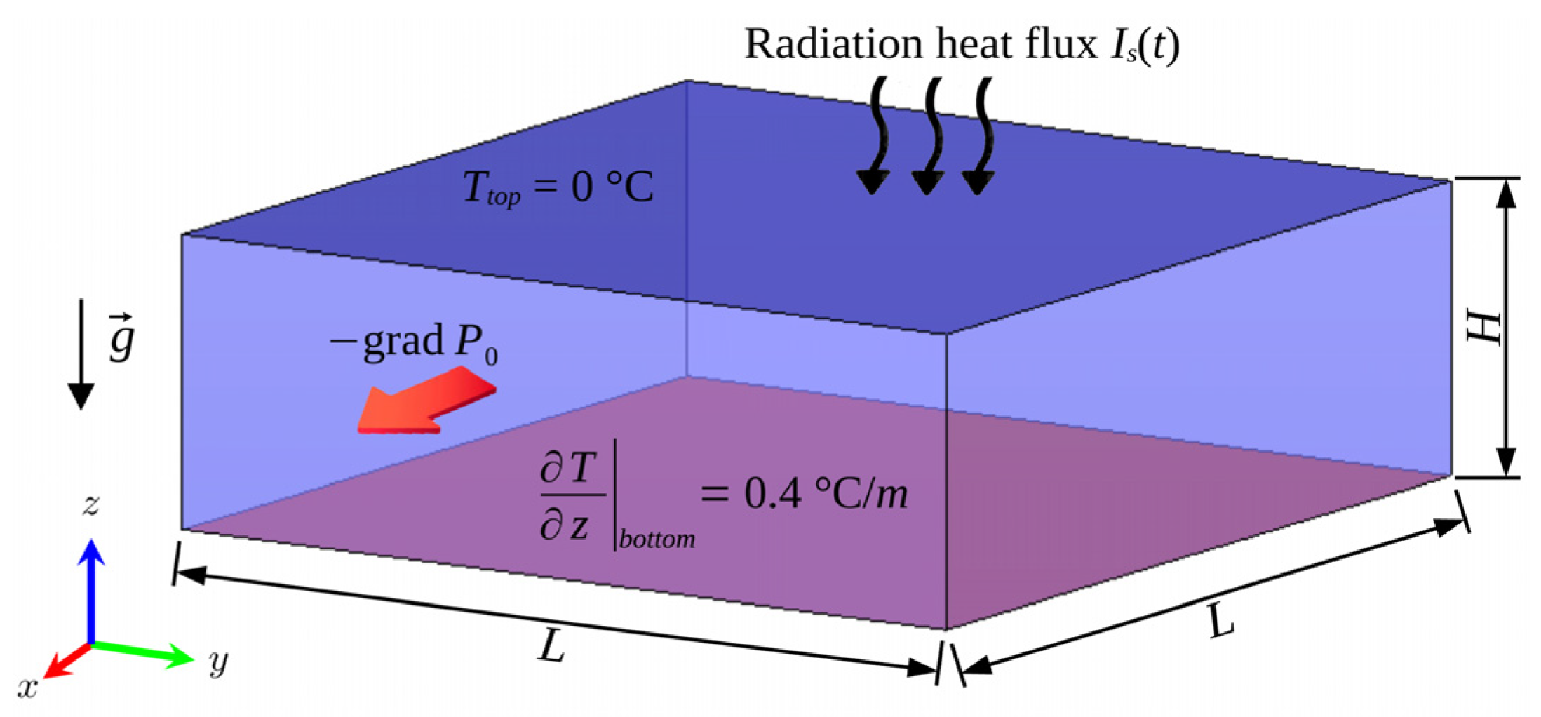
2. Problem Definition and Computational Aspects

The problem definition is very similar to that used in our previous numerical investigations [40,41]. Here, we briefly describe the main features of the problem definition. The computational domain is a rectangular cuboid with dimensions L × L × H, see Figure 1. As shown in the cited papers, a domain of size 9.6 m × 9.6 m × 6.4 m is suitable for obtaining results with acceptable accuracy.

The temperature at the top was fixed at 0 °C. The bottom had a constant heat flow applied (0.4 °C/m). Boundary conditions at the lateral planes of the computation domain were set to periodic conditions, imitating a continuous domain. The top surface was defined as no-slip wall. At the lower boundary, the free-slip condition was specified. The initial conditions reflected an equilibrium state with zero velocity and the linear temperature profile ranging from 0 °C at the top to 2.56 °C at the bottom, matching the boundary conditions.

Turbulent motion and heat transfer were described by Navier-Stokes equations for incompressible fluid in the Boussinesq approximation:

$$\nabla ·\overrightarrow{V}=0$$

(1)

$$\frac{\partial \overrightarrow{V}}{\partial t}+\left(\overrightarrow{V}·\nabla \right)\overrightarrow{V}=-\frac{1}{\rho }\left(\nabla p+\mathrm{grad}{P}_0\right)+\beta \left(T_0-T\right)\overrightarrow{g}+\nu {\nabla }^2\overrightarrow{V}$$

(2)

$$\frac{\partial T}{\partial t}+\left(\overrightarrow{V}·\nabla \right)T=\alpha {\nabla }^{2}T+\frac{\partial I}{\partial z}$$

(3)

where $\overrightarrow{V}=\left(V_x,V_y,V_z\right)$ is the velocity vector, t is the physical time, p is the pressure, T is the water temperature, ρ is the water density, $\overrightarrow{g}$ is the gravity vector, T₀ = T₀(z) is the initial linear temperature profile under hydrostatic equilibrium, α is the thermal diffusivity coefficient, ν is the kinematic viscosity coefficient, β is the thermal expansion coefficient, ∂I/∂z is the volumetric heat source, and gradP₀ is the external pressure gradient oriented along the x-axis.

The thermophysical parameters were taken for pure water at 2 °C. The coefficients a and ν were constant. The thermal expansion coefficient was calculated as β = b₁·(T – T_md), where b₁ = 1.65·10⁻⁵ K⁻², T_md = 3.84 °C.

For radiative heating, a two-band approximation of the attenuation law was used:

I(z, t) = I_s(t) [a₁exp(−γ₁z) + a₂exp(−γ₂z)]

(4)

where I(z, t) is the kinematic flux of penetrating solar radiation, i.e., the heat flux divided by the density and specific heat capacity of water. The volumetric heat source was added to the energy equation (∂I/∂z). The radiation heat flux at the top boundary, I_s, was the prescribed periodic function, formulated according to the experimental data [22,40].

To estimate the effect of the lateral flow on the structure of the convection in the CML, a series of calculations was carried out with a constant pressure gradient oriented along the x-axis. The pressure gradient varied from 3.28·10⁻⁶ Pa/m to 3.28·10⁻⁴ Pa/m. The values of the pressure gradient were calculated by the Darcy–Weisbach equation according to the characteristic mean velocity of the horizontal flow in the fully established turbulent regime of the flow in the 2D channel, whose size is equal to double the computational domain height (for the Darcy friction factor we use approximation $\lambda ={\left(1.8log\mathrm{Re}-1.64\right)}^{-2}$). Thus, the value 3.28·10⁻⁶ Pa/m corresponds to about 1 mm/s, and the value 3.28·10⁻⁴ Pa/m corresponds to several centimeters per second. The pressure gradient in all calculations was set as starting from 6 a.m. of the 4th day when the CML is fully formed, as shown in our previous study [40]. Thus, the calculations for the first 78 h were carried out with the original settings (without external pressure gradient).

Numerical simulations were conducted using the in-house finite-volume CFD-code SINF/Flag-S developed at the Higher School of Applied Mathematics and Computational Physics, Peter the Great St. Petersburg Polytechnic University. The code operates with an unstructured grid using the Finite Volume Method. The Implicit LES (ILES) approach was employed. The SIMPLEC algorithm was used to advance in time. For spatial discretization of convective flows, we used the QUICK scheme, which was nominally of third-order accuracy. The central-difference scheme of second-order accuracy was applied for approximation of the diffusion terms.

The computational grid used here consisted of hexagonal elements. The number of elements was 27 mln cells (300 × 300 × 300 cells). The grid was clustered to the top wall. The time step was 2.5 s. The study of the grid influence on the velocity and temperature fields, as well as changes in pulsations of velocity components, was presented earlier in papers [40,41], and it was shown that the grid with 27 mln cells is enough for obtaining a grid-independent solution both for the mean and RMS flow characteristics.

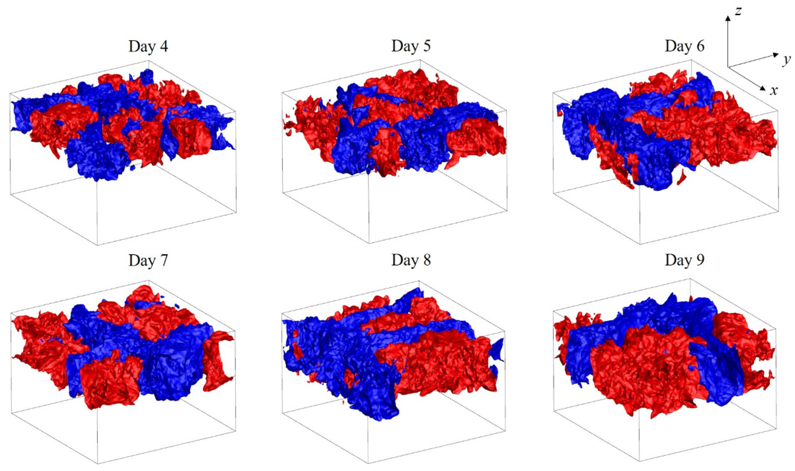
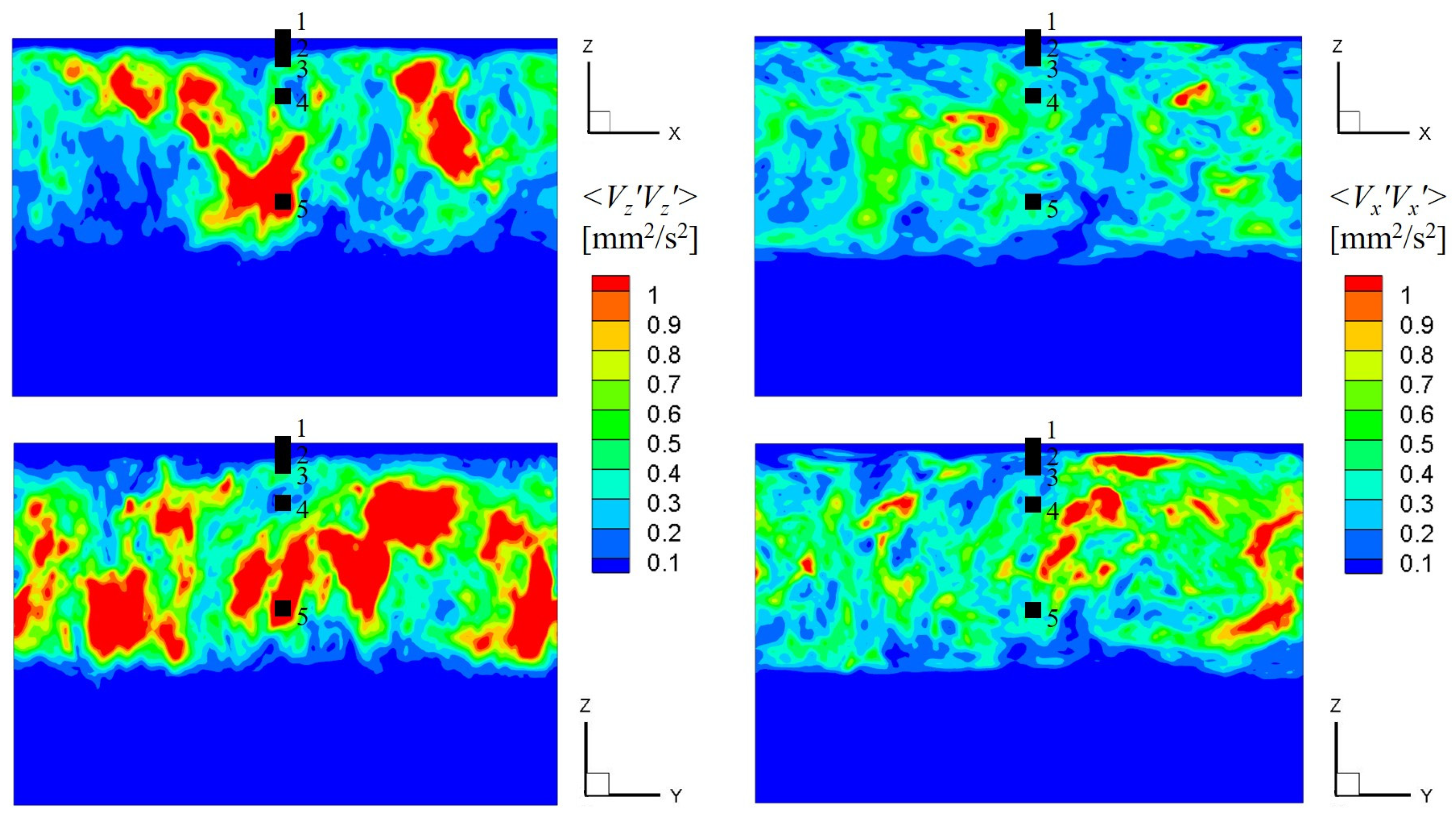
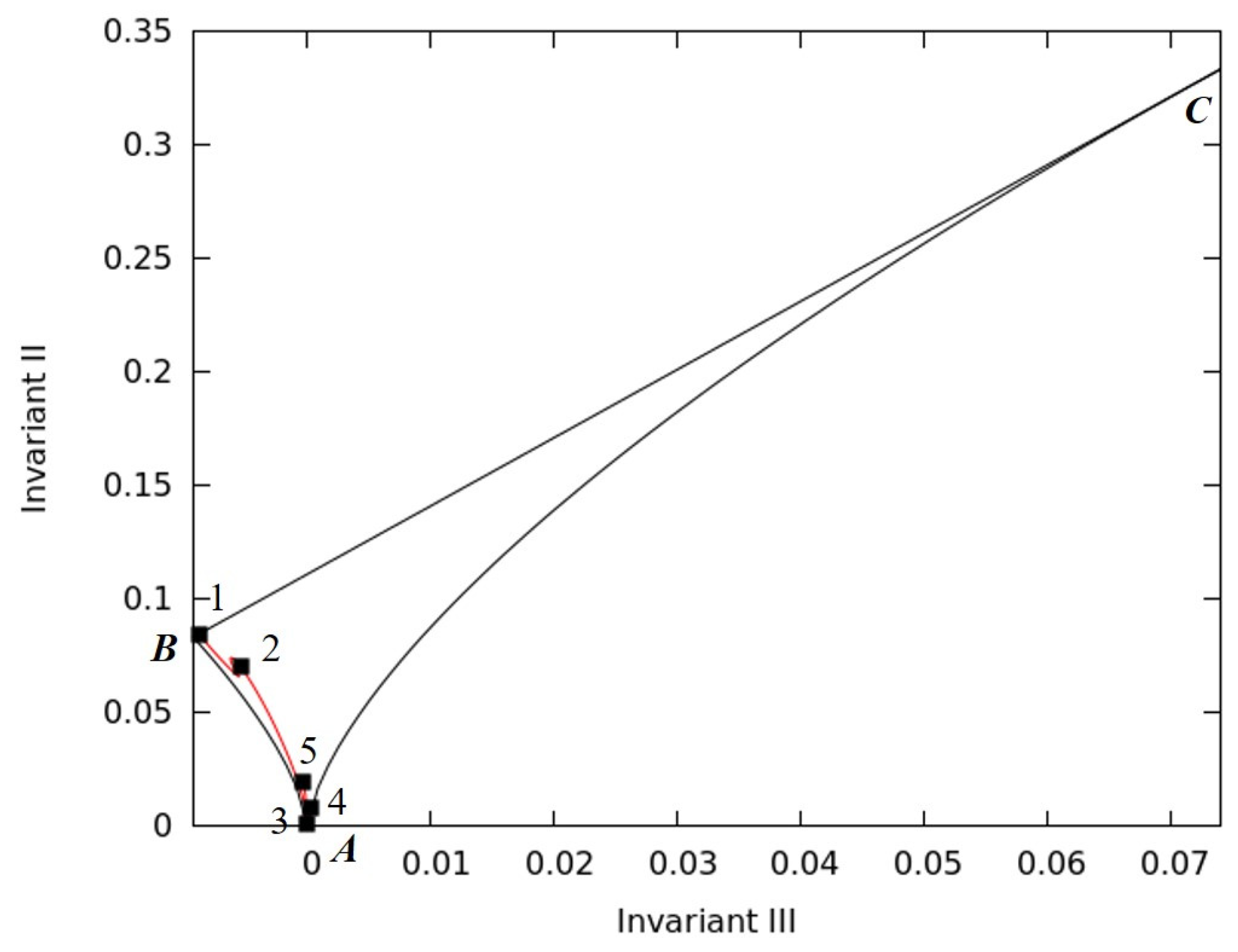
3. Results and Discussion

3.1. Radiatively Driven Convection in the Variant of Zero Lateral Pressure Gradient

In this section, we present the results for the setup with a zero-pressure gradient. These results were widely reported in previous articles [40,41]. We briefly describe the main features of RDC in the absence of lateral flow. The simulation start time is 6 a.m. when the solar radiation flux begins to increase. In the first few hours, the water layer near the top boundary warms up, and convection arises. At this stage, the CML begins to develop.

In our previous study [40], we analyzed the structure of the flow, temporary changes in velocity and temperature in CML, as well as changes in temperature along the depth and the integral characteristics: the rate of deepening of the CML and the increase in its temperature. In this study, firstly we illustrate the evolution of spatial structures within the CML over several days with zero lateral pressure gradient, and then we investigate the evolution of CML with different values of lateral pressure gradient. For a more detailed investigation of spatio-temporal flow heterogeneity and turbulence archetypes, here we also present the results of an invariant analysis (see below).

Our previous LES results [40] revealed that convective cells are an element of the spatial structure of CML, which are formed inside the CML within 3–4 days from the start of the kinematic heat flux at the upper boundary of the computational domain. For better visualization of the spatial structure of CML and its evolution during several days, the isosurfaces of the vertical velocity component corresponding to ascending and descending flows are shown in Figure 2 from the fourth to the ninth day. The width of the computational domain is 9.6 m, so it can be argued that the horizontal size of these cells can reach several meters. As a result of the gradual accumulation of heat entering the system, the temperature and thickness of the CML as well as the intensity of convective motion increase day by day. This, in turn, leads to a growth in the characteristic size of convective cells. In particular, the size of the cells on the ninth day is approximately twice that of the cell size on the fourth day.

Figure 3 presents the fluctuations of the velocity components in different cross-sections in the middle of the eighth day. We see that pulsations take place only in the CML; there is no movement in the underlying stratified layer.

As the thickness of the CML and the size of large-scale structures increase, the fluctuation characteristics also increase. Where lateral flow is absent, vertical fluctuations distinctly prevail over horizontal ones. Their distribution through the entire thickness of the CML is almost homogeneous.

To illustrate the turbulence anisotropy inside the CML, we performed an Anisotropic Invariant Map (AIM) analysis [44,45,46,47], which is based on calculation of the second II = a_ija_ji/2 and third III = a_ija_jla_li/3 invariants of the anisotropy tensor a_ij = ⟨V_i′V_j′⟩/(2k) – δ_ij/3 (V_i′ is the pulsation of the i-th velocity component; angular brackets is time averaging; k is the turbulence kinetic energy; summation on repeated indexes henceforward). Each state of turbulence is represented by a point on the AIM, all physically acceptable states form the so-called Lumley triangle, where the upper bound is described by the equation II = 1/9 + 3III and corresponds to the 2D turbulence, the lateral bounds (described by the equation II = 3(III/2)^2/3) represent the axisymmetric turbulence: “rod-like” or “disk-like” pulsations [48]. The point (0, 0) corresponds to the isotropic turbulence.

Figure 4 shows the AIM in the “II-III invariants” coordinates, obtained by averaging in the horizontal planes of time-averaged invariants on the eighth day from 2 p.m. to 3 p.m.; the red curve corresponds to the change in the invariants along the vertical coordinate, the black symbols correspond to horizontal planes passing through the points shown in Figure 3. Points 1 and 2 are located inside the boundary layer near the top boundary, point 3 is located in the upper part of the CML, point 4 is located near the center of the CML, and point 5 is selected near the lower part of CML. Comparing the corresponding AIM obtained for the convection in the titled cylinder (see Figure 9 in [44]) and the internally heated convection (see Figure 17 in [44]), one can see certain similarities in the behavior of the anisotropy: the AIM lies near the left boundary of the Lumley triangle, so turbulence near the top of the CML is nearly 2D axisymmetric with a predominance of pulsations of the one (vertical) component. Inside the CML, turbulence remains axisymmetric “rod-like” but with a tendency to be isotropic (see Figure 1 in [44]). The similarity of the AIMs for the considered cases (RDC considered in this paper and two cases of Rayleigh–Bénard-type convection, which were analyzed in [44]) corroborates the proximity of the large-scale turbulent structures obtained in both cases; these large-scale structures (convective cells) are typical for Rayleigh–Bénard-type convection.

3.2. Effect of a Lateral Pressure Gradient

The pressure gradient was set in all variants at 6 a.m. on the fourth day, that is, after 72 h of the calculation. A fully developed CML, due to the radiation pumping according to equation (4), had managed to form by this time. Firstly, the calculations were carried out with the relatively high value of gradP₀ equal to 3.28·10⁻⁴ Pa/m, corresponding to the lateral flow velocity of several centimeters per second in an established regime. In the middle of the day (9 h after the start of the gradP₀ setting, at 3 p.m.), a decrease in the expression of large-scale convective cells was observed (Figure 5, Day 1). Here and below, the counting of days begins from the moment the pressure gradient is specified. Thus, 3 p.m. on the first day (see Figure 5) in total corresponds to 81 h of calculations (three days with the initial settings and 9 h with the gradP₀ settings). In the following days, further restructuring of the flow is observed with the formation of elongated “two-dimensional” rolls oriented along the superimposed horizontal flow (Figure 5, Day 2). Further development of convection in the layer, accompanied by an increase in longitudinal velocity, led to the disintegration of large-scale structures and a prevalence of small-scale turbulence (Figure 5, Day 3). The evolution of the flow obtained in the calculations with and without the pressure gradient in similar hours of 4–6 days of calculation can be traced by comparing the results shown in Figure 2 and Figure 5.

Calculations with lower values of the pressure gradient generally illustrate a similar, although longer, transformation of the spatial structure inside the CML. Obviously, the lower the gradP₀, the lower the lateral flow velocity, which leads to a later transition from large-scale cells to elongated “two-dimensional” rolls. For example, with gradP₀ equal to 3.28·10⁻⁵ Pa/m, the transition to elongated structures occurred on the second day, while large-scale structures were still observed on the first day (Figure 6). For even lower values of gradP₀ equal to 6.56·10⁻⁶ Pa/m and 3.28·10⁻⁶ Pa/m, illustrated in Figure 7 and Figure 8, the transition to “two-dimensional” rolls happened on the fifth and ninth days, respectively. In the previous days, due to the relatively low lateral flow velocities, the flow structure in the CML was almost the same as in the case without an external lateral pressure gradient. The structure of the formed elongated rolls is similar to the well-known Langmuir circulation [2]. At this time, we cannot give a specific cause for the transition from the convective cells to the elongated 2D rolls. There are some considerations concerning the numerical formulation of the problem, where the ideal periodic conditions are specified on the lateral bounds: the posed non-uniformity (pressure gradient) leads to the appearance of a preferred direction. Thus, in the formulation under consideration, we expect a transition from cells to two-dimensional rolls even with a very small applied lateral pressure gradient. In real conditions, there should be a critical value of the lateral pressure gradient, below which the transition is not observed. Note that in variants with lower values of the pressure gradient, we did not observe the disintegration of the rolls and transition to small-scale turbulence as in the case with the highest pressure gradient. Perhaps the reason is that the model time was insufficient for variants with smaller pressure gradients, and if the calculation duration was longer, we would see the disintegration of the rolls at some point in time.

Figure 9a,b illustrates the distribution of time-averaged velocity components along the central vertical line at gradP₀ = 3.28·10⁻⁵ Pa/m (fifth day from the setting of the external pressure gradient). We see that the horizontal flow velocity is maximal in the bottom stratified layer, reaching about 12 mm/s. In the CML, convective cells interact with superimposed lateral motion, which leads to a significant decrease in the horizontal velocity component. The vertical flow velocity reaches its maximum inside the CML; in the stratified layer, the vertical component is close to zero.

The instantaneous horizontally averaged temperature profiles are presented in Figure 9c for two variants corresponding to the pressure gradients 3.28·10⁻⁵ Pa/m and 3.28·10⁻⁴ Pa/m. In the case of gradP₀ = 3.28·10⁻⁵ Pa/m and less, the temperature profile has a characteristic form of RDC with distinct CML boundaries. The large pressure gradient leads to significant changes in profile: shear stress between horizontal flow in a stable stratified layer and CML leads to strong turbulent mixing in the lower part of the CML. These changes in flow make it difficult to determine such characteristics of the CML as its depth and temperature. Thus, our simulation shows that at a relatively large pressure gradient, the structure of the flow and CML can significantly transform over time, and such effects need to be studied in detail in the future.

In Figure 10, one can see the “imprints” of elongated structures on the fields of fluctuations of the velocity components in vertical planes. The results are given for the case corresponding to gradP₀ = 3.28·10⁻⁵ Pa/m in the middle of the fifth day after setting the pressure gradient. We see that in the plane oriented along the x-axis (upper row in Figure 10), “two-dimensional” rolls are observed very clearly. The illustrations in the perpendicular plane (bottom row of Figure 10) are more inhomogeneous and show the distribution of elongated rolls (along the x-axis) in the direction of the y-axis.

Since the distribution of fluctuations in the case of setting the pressure gradient is clearly heterogeneous across the CML, it makes sense to compare the evolution of fluctuations for the two variants (initial zero-gradient and taking into account lateral flow) at different depths. Figure 11 and Figure 12 show such comparison at depths of 1.5 and 3.5 m, corresponding to the middle of the CML and its lower boundary. When considering the case with lateral flow, the value of the pressure gradient was taken equal to 3.28·10⁻⁵ Pa/m. It can be seen that the imposition of a pressure gradient leads to an increase in the velocity fluctuations inside the CML for both depths under consideration. However, due to the inhomogeneity of their distributions, the ratio between the horizontal and vertical pulsations can vary significantly across depths. In particular, in the middle of the CML (depth 1.5 m, Figure 11), vertical pulsations prevail over horizontal ones both for the zero-gradient case and with a lateral gradient present. In Figure 12, which shows the distribution of pulsations near the CML lower boundary, we see the opposite correlation and a prevalence of horizontal pulsations for both variants of calculations.

Lateral flows of various nature are often revealed in ice-covered lakes [33,34,49,50], which certainly increases the fluctuations of the horizontal velocity components. As RDC develops, an increase in vertical velocity pulsations can be expected. The problem, however, is that there are very few field measurements of velocity components during RDC that cover the entire mixed layer. Velocity measurements covered the entire thickness of the CML in Petrozavodsk Bay of Lake Onega in mid-March 2016. According to these measurements, the maximum values of horizontal components correspond to the upper and lower boundaries of the CML, while in the middle of this layer horizontal velocity components decrease [33]. The vertical component was smaller than the horizontal ones and showed a pronounced increase in the daytime in correlation with the radiation flux.

On the contrary, in small lakes or ponds without the lateral pressure gradient, the main driving force of mixing during RDC is gravitational instability, and a predominance of vertical velocity pulsations can be expected. In such small lakes and ponds, convective cells remain in a stable horizontal position, which can be indirectly confirmed by the star-shaped structures on the ice surface [22]. A predominance of vertical pulsation is also typical for the Rayleigh-Bénard type convection (e.g., see [44]).

Admittedly, field measurements that would make it possible to understand exactly how the pulsations of horizontal and vertical velocities change across the thickness of the CML are still extremely limited.

The transition from convective cells to 2D rolls can be illustrated by AIM analysis: for the case with external pressure gradient gradP₀ = 3.28·10⁻⁴ Pa/m, we also evaluate horizontally averaged AIMs. In Figure 13, AIMs for different days are presented. One can see that on the first day after involving the pressure gradient, the AIM becomes different from the one shown in Figure 4 for the zero-gradient case, but this difference is minor: in most of the CML, the turbulence anisotropy is similar for both cases. In the next days, however, the AIM differs significantly; the red line corresponds to anisotropy with a prevalence of one (horizontal) pulsation in the middle of the CML and a tendency towards 2D turbulence near the top and bottom of the CML (Figure 13a). A similar pattern of 2D-3D transformation is observed for other values of the pressure gradient (Figure 13b,c). Previously, we discovered changes in the turbulence regime in the CML of Lake Vendyurskoe, when multiple 2D-3D transitions recurred every day [34]. These previous studies, however, did not detect changes in the structure of turbulence in the CML with irreversible transition from cells to rolls. As it was mentioned earlier, such a transition, even in the case of a relatively small pressure gradient, can be associated with an “ideal” numerical problem formulation with the imposition of periodic boundary conditions.

To compare the results of the numerical simulation with field observations, we, as before in [40], calculate the integral parameters of the CML. Cumulative integral heating (Q), temperature (TCML), and depth (HCML) increments are calculated as:

$$Q=I_0\rho C_p{\int }_o^{t}sin\left(2\pi \frac{t}{T^{*}}\right)dt$$

(5)

TCML = <T> − <T_CML,0>

(6)

HCML = h − h_CML,0

(7)

where h_CML,0 and <T_CML,0> are the average depth and temperature of the CML at the time of its formation.

The dependencies of TCML and HCML on cumulative heating Q are illustrated in Figure 14 for variants with zero-pressure gradient and with relatively small pressure gradients. As shown previously in [40], the numerical simulation for the initial case with a zero-pressure gradient demonstrates a good correlation with the observed CML dynamic in Lake Vendyurskoe in different years. For lateral pressure gradients less or equal to 3.28·10⁻⁵ Pa/m, we did not observe significant changes in the evolution of the depth of the lower boundary of the CML and its temperature. As mentioned above, at gradP₀ = 3.28·10⁻⁴ Pa/m there is a noticeable change in the temperature profile, so the CML is not expressed so clearly; therefore, these data are not shown in Figure 14.

Thus, numerical simulation showed that the lateral gradient has a virtually small effect on the deepening of the CML. This result is ambiguous and requires further study. Doubts arise from the fact that the rate of vertical mixing in lakes may be noticeably reduced when lateral currents develop. In some lakes, significant late-winter meltwater influx generates lateral transport that may limit the penetration of convective mixing. This effect was described by Cortés and MacIntyre [49] for the small Arctic Lake Toolik. Also, the influence of lateral transport on the development of RDC was considered for Lake Pääjärvi (Finland) by Salonen et al. [50]: based on nine years of field observations, the authors showed that the contribution of horizontal and vertical mixing varied among years, and in one of the investigated spring seasons, horizontal convection dominated.

4. Conclusions

The results of the numerical simulation of RDC in a small ice-covered lake with and without lateral pressure gradient are presented. Our calculations showed that with a zero-pressure gradient, there is a number of convective cells with zones of ascending and descending flow inside the CML formed 3–4 days after the start of kinematic heat flux at the upper boundary of the computational domain.

Numerical simulations performed with various pressure gradient values show that the presence of even a relatively small lateral pressure gradient leads to a transition from large-scale convective cells to elongated “two-dimensional” rolls. The change in the CML’s turbulence patterns under a lateral pressure gradient is confirmed by the AIM analysis.

These results prove the importance of lateral transport in the formation of the CML structure. However, the simulated patterns of a one-way transition from convective cells to rolls have not yet been verified by field measurements in lakes. To date, we are not aware of any cases of irreversible cell-to-roll transitions observed in the CML of seasonally frozen lakes. Also, the next stage—the break-up of the rolls and the transition to small-scale turbulence—has not yet been registered in field measurements. Such changes in CML structure can be expected in ice-covered lakes with significant lateral transport, for example, in lakes that are part of lake–river systems. In the future, measurements in high-flow lakes will be carried out in order to identify such a transformation of the CML structure.

The dependence of the temperature and depth increments of the CML on cumulative heating in the calculations with a zero-pressure gradient correlated well with the field observations. The results of the numerical simulation with a pressure gradient setting barely differed from the initial, zero-gradient variant for a gradP₀ value less than or equal to 3.28·10⁻⁵ Pa/m. As the pressure gradient increases and, as a consequence, the horizontal velocity increases, large-scale rolls are suppressed, and the CML changes, which leads to difficulties in detecting its lower boundary.

Important future research directions include further integration of field observations and numerical simulation for evaluating CML parameters and structure evolution under changing external and internal factors.

References

1. Farmer, D.M.; Carmack, E. Wind mixing and restratification in a lake near the temperature of maximum density. J. Phys. Oceanogr. 1981, 11, 1516–1533. [Google Scholar] [CrossRef]
2. Wüest, A.; Lorke, A. Small-scale hydrodynamics in lakes. Annu. Rev. Fluid Mech. 2003, 35, 373–412. [Google Scholar] [CrossRef]
3. Bouffard, D.; Wüest, A. Convection in lakes. Annu. Rev. Fluid Mech. 2019, 51, 189–215. [Google Scholar] [CrossRef]
4. Weiss, R.; Carmack, E.; Koropalov, V. Deep-water renewal and biological production in Lake Baikal. Nature 1991, 349, 665–669. [Google Scholar] [CrossRef]
5. González-Salgado, D.; Noya, E.G.; Lomba, E. Simulation and theoretical analysis of the origin of the temperature of maximum density of water. Fluid Phase Equilibria 2022, 560, 113515. [Google Scholar] [CrossRef]
6. Jonas, T.; Stips, A.; Eugster, W.; Wüest, A. Observations of a quasi shear-free lacustrine convective boundary layer: Stratification and its implications on turbulence. J. Geophys. Res. 2003, 108, 3328. [Google Scholar] [CrossRef]
7. Ghane, A.; Boegman, L. Turnover in a small Canadian shield lake. Limnol. Oceanogr. 2021, 66, 3356–3373. [Google Scholar] [CrossRef]
8. Farmer, D.M. Penetrative convection in the absence of mean shear. Q. J. R. Meteorol. Soc. 1975, 101, 869–891. [Google Scholar] [CrossRef]
9. Jonas, T.; Terzhevik, A.Y.; Mironov, D.V.; Wüest, A. Radiatively driven convection in an ice-covered lake investigated by using temperature microstructure technique. J. Geophys. Res. 2003, 108, 3183. [Google Scholar] [CrossRef]
10. Austin, J.A. Observations of radiatively driven convection in a deep lake. Limnol. Oceanogr. 2019, 64, 2152–2160. [Google Scholar] [CrossRef]
11. Cannon, D.J.; Troy, C.D.; Liao, Q.; Bootsma, H.A. Ice-Free Radiative Convection Drives Spring Mixing in a Large Lake. GRL 2019, 46, 6811–6820. [Google Scholar] [CrossRef]
12. Carmack, E.C.; Weiss, R.F. Convection in Lake Baikal: An Example of Thermobaric Instability; Chu, P.C., Gascard, J.C., Eds.; Elsevier Oceanography Series; Elsevier: Amsterdam, The Netherlands, 1991; Volume 57, pp. 215–228. [Google Scholar] [CrossRef]
13. Boehrer, B.; Golmen, L.; Løvik, J.E.; Rahn, K.; Klaveness, D. Thermobaric stratification in very deep Norwegian freshwater lakes. J. Great Lakes Res. 2013, 39, 690–695. [Google Scholar] [CrossRef]
14. Carmack, E.; Vagle, S. Thermobaric processes both drive and constrain seasonal ventilation in deep Great Slave Lake, Canada. J. Geophys. Res. Earth Surf. 2021, 126, e2021JF006288. [Google Scholar] [CrossRef]
15. Austin, J.; Hill, C.; Fredrickson, J.; Weber, G.; Weiss, K. Characterizing temporal and spatial scales of radiatively driven convection in a deep, ice-free lake. Limnol. Oceanogr. 2022, 67, 2296–2308. [Google Scholar] [CrossRef]
16. Kelley, D. Convection in ice-covered lakes: Effects on algal suspension. J. Plankton Res. 1997, 19, 1859–1880. [Google Scholar] [CrossRef]
17. Pernica, P.; North, R.L.; Baulch, H.M. In the cold light of day: The potential importance of under-ice convective mixed layers to primary producers. Inland Waters 2017, 7, 138–150. [Google Scholar] [CrossRef]
18. Huang, W.; Zhang, Z.; Li, Z.; Lepparanta, M.; Arvola, L.; Song, S.; Huotari, J.; Lin, Z. Under-ice dissolved oxygen and metabolism dynamics in a shallow lake: The critical role of ice and snow. Water Resour. Res. 2021, 57, e2020WR027990. [Google Scholar] [CrossRef]
19. Bouffard, D.; Zdorovennova, G.; Bogdanov, S.; Efremova, T.; Lavanchy, S.; Palshin, N.; Terzhevik, A.; Vinnå, L.R.; Volkov, S.; Wüest, A.; et al. Under-ice convection dynamics in a boreal lake. Inland Waters 2019, 9, 142–161. [Google Scholar] [CrossRef]
20. Suarez, E.L.; Tiffay, M.-C.; Kalinkina, N.; Tchekryzheva, T.; Sharov, A.; Tekanova, E.; Syarki, M.; Zdorovennov, R.E.; Makarova, E.; Mantzouki, E.; et al. Diurnal variation in the convection-driven vertical distribution of phytoplankton under ice and after ice-off in large Lake Onego (Russia). Inland Waters 2019, 9, 193–204. [Google Scholar] [CrossRef]
21. Yang, B.; Wells, M.G.; Li, J.; Young, J. Mixing, stratification, and plankton under lake-ice during winter in a large lake: Implications for spring dissolved oxygen levels. Limnol. Oceanogr. 2020, 65, 2713–2729. [Google Scholar] [CrossRef]
22. Mironov, D.; Terzhevik, A.; Kirillin, G.; Jonas, T.; Malm, J.; Farmer, D. Radiatively driven convection in ice-covered lakes: Observations, scaling, and a mixed layer model. J. Geophys. Res. 2002, 107, 1–16. [Google Scholar] [CrossRef]
23. Kirillin, G.; Terzhevik, A. Thermal instability in freshwater lakes under ice: Effect of salt gradients or solar radiation? Cold Reg. Sci. Tech. 2011, 65, 184–190. [Google Scholar] [CrossRef]
24. Mironov, D.V.; Terzhevik, A.Y. Spring Convection in Ice-Covered Freshwater Lakes. Izv. Atmos. Ocean. Phys. 2000, 36, 627–634. [Google Scholar]
25. Mironov, D.V.; Danilov, S.D.; Olbers, D.J. Large-eddy simulation of radiatively-driven convection in ice covered lakes. In Proceedings of the Sixth Workshop on Physical Processes in Natural Waters, Girona, Spain, 27–29 June 2001; Casamitjana, X., Ed.; University of Girona: Girona, Spain, 2001; pp. 71–75. [Google Scholar]
26. Ulloa, H.N.; Winters, K.B.; Wüest, A.; Bouffard, D. Differential heating drives downslope flows that accelerate mixed-layer warming in ice-covered waters. Geophys. Res. Lett. 2019, 46, 13872–13882. [Google Scholar] [CrossRef]
27. Ramón, C.L.; Ulloa, H.N.; Doda, T.; Winters, K.B.; Bouffard, D. Bathymetry and latitude modify lake warming under ice. Hydrol. Earth Syst. Sci. 2021, 25, 1813–1825. [Google Scholar] [CrossRef]
28. Kirillin, G.; Aslamov, I.; Leppäranta, M.; Lindgren, E. Turbulent mixing and heat fluxes under lake ice: The role of seiche oscillations. Hydrol. Earth Syst. Sci. 2018, 22, 6493–6504. [Google Scholar] [CrossRef]
29. Kiili, M.; Pulkkanen, M.; Salonen, K. Distribution and development of under-ice phytoplankton in 90-m deep water column of Lake Päijänne (Finland) during spring convection. Aquat. Ecol. 2009, 43, 707–713. [Google Scholar] [CrossRef]
30. Vehmaa, A.; Salonen, K. Development of phytoplankton in Lake Pääjärvi (Finland) during under-ice convective mixing period. Aquat. Ecol. 2009, 43, 693–705. [Google Scholar] [CrossRef]
31. Jansen, J.; MacIntyre, S.; Barrett, D.C.; Chin, Y.-P.; Cortés, A.; Forrest, A.L.; Hrycik, A.R.; Martin, R.; McMeans, B.C.; Rautio, M.; et al. Winter limnology: How do hydrodynamics and biogeochemistry shape ecosystems under ice? J. Geophys. Res. Biogeosci. 2021, 126, e2020JG006237. [Google Scholar] [CrossRef]
32. Wüest, A.; Pasche, N.; Ibelings, B.; Sharma, S.; Filatov, N. Life under ice in Lake Onego (Russia)—An interdisciplinary winter limnology study. Inland Waters 2019, 9, 125–129. [Google Scholar] [CrossRef]
33. Bogdanov, S.; Zdorovennova, G.; Volkov, S.; Zdorovennov, R.; Palshin, N.; Efremova, T.; Terzhevik, A.; Bouffard, D. Structure and dynamics of convective mixing in Lake Onego under ice-covered conditions. Inland Waters 2019, 9, 177–192. [Google Scholar] [CrossRef]
34. Bogdanov, S.; Maksimov, I.; Zdorovennov, R.; Palshin, N.; Zdorovennova, G.; Smirnovsky, A.; Smirnov, S.; Efremova, T.; Terzhevik, A. Anisotropic Turbulence in the Radiatively Driven Convective Layer in a Small Shallow Ice-Covered Lake: An Observational Study. Bound.-Layer Meteorol. 2023, 187, 295–310. [Google Scholar] [CrossRef]
35. Martinat, G.; Xu, Y.; Grosch, C.E.; Tejada-Martínez, A.E. LES of turbulent surface shear stress and pressure-gradient-driven flow on shallow continental shelves. Ocean Dyn. 2011, 61, 1369–1390. [Google Scholar] [CrossRef]
36. Crosman, E.T.; Horel, J.D. Idealized Large-Eddy Simulations of Sea and Lake Breezes: Sensitivity to Lake Diameter, Heat Flux and Stability. Bound.-Lay. Meteorol. 2012, 144, 309–328. [Google Scholar] [CrossRef]
37. Santo, M.A.; Toffolon, M.; Zanier, G.; Giovannini, L.; Armenio, V. Large eddy simulation (LES) of wind-driven circulation in a peri-alpine lake: Detection of turbulent structures and implications of a complex surrounding orography. J. Geophys. Res. Oceans 2017, 122, 4704–4722. [Google Scholar] [CrossRef]
38. Zhang, Y.; Huang, Q.; Ma, Y.; Luo, J.; Wang, C.; Li, Z.; Chou, Y. Large eddy simulation of boundary-layer turbulence over the heterogeneous surface in the source region of the Yellow River. Atmos. Chem. Phys. 2021, 21, 15949–15968. [Google Scholar] [CrossRef]
39. Grace, A.P.; Stastna, M.; Lamb, K.G.; Scott, K.A. Numerical simulations of the three-dimensionalization of a shear flow in radiatively forced cold water below the density maximum. Phys. Rev. Fluids 2022, 7, 023501. [Google Scholar] [CrossRef]
40. Smirnov, S.; Smirnovsky, A.; Zdorovennova, G.; Zdorovennov, R.; Palshin, N.; Novikova, I.; Terzhevik, A.; Bogdanov, S. Water Temperature Evolution Driven by Solar Radiation in an Ice-Covered Lake: A Numerical Study and Observational Data. Water 2022, 14, 4078. [Google Scholar] [CrossRef]
41. Smirnovsky, A.A.; Smirnov, S.I.; Bogdanov, S.R.; Palshin, N.I.; Zdorovennov, R.E.; Zdorovennova, G.E. Numerical Simulation of Turbulent Mixing in a Shallow Lake for Periods of Under-Ice Convection. Water Resour. 2023, 50, 622–632. [Google Scholar] [CrossRef]
42. Chang, Y.; Scotti, A. Characteristic scales during the onset of radiatively driven convection: Linear analysis and simulations. J. Fluid Mech. 2023, 973, A14. [Google Scholar] [CrossRef]
43. Noto, D.; Ulloa, H.; Yanagisawa, T.; Tasaka, Y. Stratified horizontal convection. J. Fluid Mech. 2023, 970, A21. [Google Scholar] [CrossRef]
44. Smirnov, S.; Smirnovsky, A.; Bogdanov, S. The Emergence and Identification of Large-Scale Coherent Structures in Free Convective Flows of the Rayleigh-Bénard Type. Fluids 2021, 6, 431. [Google Scholar] [CrossRef]
45. Lumley, J.L. Computational modeling of turbulent flows. Adv. Appl. Mech. 1978, 18, 123–176. [Google Scholar] [CrossRef]
46. Choi, K.-S.; Lumley, J.L. The return to isotropy of homogeneous turbulence. J. Fluid Mech. 2001, 436, 59–84. [Google Scholar] [CrossRef]
47. Penna, N.; Coscarella, F.; D’Ippolito, A.; Gaudio, R. Anisotropy in the Free Stream Region of Turbulent Flows through Emergent Rigid Vegetation on Rough Beds. Water 2020, 12, 2464. [Google Scholar] [CrossRef]
48. Simonsen, A.J.; Krogstad, P.-A. Turbulent stress invariant analysis: Clarification of existing terminology. Phys. Fluids 2005, 17, 088103. [Google Scholar] [CrossRef]
49. Cortés, A.; MacIntyre, S. Mixing processes in small arctic lakes during spring. Limnol. Oceanogr. 2020, 65, 260–288. [Google Scholar] [CrossRef]
50. Salonen, K.; Pulkkanen, M.; Salmi, P.; Griffiths, R.W. Interannual variability of circulation under spring ice in a boreal lake. Limnol. Oceanogr. 2014, 56, 2121–2132. [Google Scholar] [CrossRef]
Figure 1. Scheme of the computational domain and temperature boundary conditions.
Water 15 03953 g001
Figure 2. Isosurfaces of the time-averaged vertical velocity component presented for six consecutive days for variant of zero lateral pressure gradient (|<Vz>| = 0.6 mm/s, blue structures correspond to descending currents, red structures correspond to ascending ones), the averaging was carried out from 2 p.m. to 3 p.m. of each day.
Water 15 03953 g002
Figure 3. The fields of pulsation of the velocity components in the central vertical sections: the top and the bottom rows correspond to planes xz and yz respectively; the averaging was carried out on the eighth day from 2 p.m. to 3 p.m. The points indicated by black rectangles represent the corresponding states on AIM in Figure 4.
Water 15 03953 g003
Figure 4. AIM: distribution at vertical coordinates averaged over the horizontal sections (eighth day, 3 p.m.). The black points correspond to the different depths presented in Figure 3; the point A corresponds isotropic turbulence, B—two component axisymmetric, C—“1D” turbulence; the black line BC corresponds “2D” turbulence, AC—axisymmetric “rod-like”, AB—axisymmetric “disk-like”.
Water 15 03953 g004
Figure 5. Isosurfaces of the time-averaged vertical velocity component presented for three consecutive days (|<Vz>| = 0.4 mm/s, blue structures correspond to descending currents, yellow structures correspond to ascending ones); gradP0 = 3.28·10−4 Pa/m. Here and in Figure 6, Figure 7 and Figure 8 the averaging was carried out from 2 p.m. to 3 p.m. of each day.
Water 15 03953 g005
Figure 6. Isosurfaces of the time-averaged vertical velocity component presented for three consecutive days (|<Vz>| = 0.6 mm/s); gradP0 = 3.28·10−5 Pa/m. Here and in Figure 7 and Figure 8 blue structures correspond to descending currents, red structures correspond to ascending ones.
Water 15 03953 g006
Figure 7. Isosurfaces of the time-averaged vertical velocity component presented for three consecutive days (|<Vz>| = 0.6 mm/s); gradP0 = 6.56·10−6 Pa/m.
Water 15 03953 g007
Figure 8. Isosurfaces of the time-averaged vertical velocity component presented for three consecutive days (|<Vz>| = 0.6 mm/s); gradP0 = 3.28·10−6 Pa/m.
Water 15 03953 g008
Figure 9. Time-averaged horizontal velocity (a) and vertical velocity (b) profiles along the central vertical line (averaging was carried out on the fifth day from 2 p.m. to 3 p.m.); (c) instantaneous horizontally averaged temperature profile on the fifth day at 3 p.m.; the black curves correspond to gradP0 = 3.28·10−5 Pa/m, the red curve corresponds to gradP0 = 3.28·10−4 Pa/m.
Water 15 03953 g009
Figure 10. The fields of the pulsations of the velocity components in the central vertical sections: the top and the bottom rows correspond to planes xz and yz respectively; gradP0 = 3.28·10−5 Pa/m, averaging was carried out on the fifth day from 2 p.m. to 3 p.m. The points indicated by black rectangles represent the corresponding states on AIM in Figure 13.
Water 15 03953 g010
Figure 11. Evolution of horizontal and vertical turbulent pulsations at a depth of 1.5 m; the averaging was carried out over time within 1 h and over space in horizontal directions. The color tab corresponds to the fields of the pulsations shown in Figure 3 and Figure 10 (the averaging was carried out from 176 to 177 h).
Water 15 03953 g011
Figure 12. Evolution of horizontal and vertical turbulent pulsations at a depth of 3.5 m; the averaging was carried out over time within 1 h and over space in horizontal directions. The color tab corresponds to the fields of the pulsations shown in Figure 3 and Figure 10 (the averaging was carried out from 176 to 177 h).
Water 15 03953 g012
Figure 13. AIM: distribution at vertical coordinates averaged over the horizontal sections: (a) gradP0 = 3.28·104 Pa/m (day 1–3), (b) gradP0 = 3.28·105 Pa/m (fifth day; black points correspond to the different cross-sections in Figure 10), (c) gradP0 = 6.56·106 Pa/m (fifth day); the averaging was carried out from 2 p.m. to 3 p.m. on the corresponding day. The meaning of the black lines is the same as in Figure 4.
Water 15 03953 g013aWater 15 03953 g013b
Figure 14. The CML temperature (a) and depth (b) increments vs. cumulative heating.
Water 15 03953 g014
Disclaimer/Publisher’s Note: The statements, opinions and data contained in all publications are solely those of the individual author(s) and contributor(s) and not of MDPI and/or the editor(s). MDPI and/or the editor(s) disclaim responsibility for any injury to people or property resulting from any ideas, methods, instructions or products referred to in the content.