Abstract
Acquisition of continuous drift ice characteristic parameters such as ice size, shape, concentration, and drift velocity are of great importance for understanding river freezing and thawing processes. This study acquired hourly oblique images captured by a shore-based camera in the winter of 2021–2022 on the Yellow River, China. The pixel point scale method for correcting oblique images is provided. The 61 lines were measured at the calibration site and the absolute error between the measured value and the calculated value was in the range of 0.009–0.850 m, with a mean error of 0.236 m. After the correction of oblique images, the true equivalent diameter of drift ice during the freezing period ranged from 0.52–13.10 m with a mean size of 3.36 m, which was larger than that of 2.30 m during the thawing period which ranged from 0.20–12.54 m. It was found that the size of drift ice increased with time during the freezing period and decreased with time during the thawing period. The fractal dimension and roundness were used to represent drift ice shape. The fractal dimension ranged from 1.0–1.3 and the roundness ranged from 0.1–1.0. A Gaussian distribution was used to estimate drift ice size and shape distributions. There is a nonlinear relationship between ice concentration and drift velocity, which can be well expressed by the logistic function. In the future, drift ice parameters for more years and hydrometeorological data for the same time need to be accumulated, which helps to analyze the freezing and thawing patterns of river ice.
1. Introduction
River ice plays an important role in the physical, biological, and human systems in regions [1]. Drift ice is usually found in rivers during the freezing and thawing processes in the winter. In mid-November, with the arrival of cold air, the water column is supercooled, and frazil ice is generated and begins to flocculate together, rising to the water surface. As pieces of frazil ice gather around each other under freezing air temperature, drift ice is observed on the river surface [2,3,4]. In mid-March of the following year, the ice cover breaks up with increasing air and water temperature or increasing flow and water level, and the broken ice cover flows downstream by the water flow [5].
Monitoring drift ice characteristics (i.e., ice size, shape, concentration, and drift velocity) is essential for a better understanding of river ice freezing and thawing [6]. The quantitative ice feature data can help validate the results of river ice model calculations. For example, the CRISSP2D model [7,8] and the RIVICE model [9] can simulate dynamic transport (ice concertation and drift velocity) of surface ice and ice jam evolution [10] during the freezing period and mechanical breakup conditions during the thawing period. Moreover, the measured true drift ice size and shape can also be used as input for upstream boundary conditions [11] for the river ice model. Previous simulations of river ice transport used the hypothetical drift ice of one size and shape and have not considered the true distribution of drift ice in nature. Therefore, the validated model with true boundary conditions can be used to predict ice transport and ice jams in the future [12].
Understanding river freezing and thawing processes contributes to river management and climate change research. Effective river management benefits ice flood safety and social stability. In the initial freezing period, large pieces of drift ice rub against and push the riverbanks as they run around bends, potentially taking away stones that protect the bank, which causes bank erosion and instability [13,14,15,16]. Once the drift ice concentration is high enough, a juxtaposed ice cover or ice jam can begin to form at a point of river constriction where drift ice bridge and become immobile [17,18]. When the ice cover or ice jam forms, changes in river hydraulics are characterized by a doubling of wetted perimeter [15] of flow in a channel, a change in the vertical velocity distribution from a single logarithmic to a double logarithmic [19], and an increase in boundary resistance exerted on the flow. If the flow release from the upstream dam is not controlled, the water level rapidly rises or ice jam may break up, causing an ice jam flood hazard [20,21,22,23]. During the thawing period, ice cover breaks up under the thermal and hydrodynamic forces. The initial broken drift ice size is relatively large and can damage embankments during movement and may also form a short-lived ice jam in the narrows channel. Therefore, ice size, concentration, and drift velocity can be a potential influential factor in river management such as ice flood risk assessment [24] and dam flow regulation in the winter. In addition, climate change can be studied through long-term monitoring of river ice phenology [24,25,26,27] such as freeze-up start, freeze-up end, break-up start, break-up end, and total duration of the ice age. However, this paper has only collected monitoring data for one winter season and cannot be applied to climate change study. In the future, more years of data need to be collected and accumulated.
Previous studies have provided some filed methods for investigating river ice. Firstly, remote sensing is mostly used to monitor ice phenology, ice thickness, and ice dams on a large scale [28,29,30,31]. In general, common high-resolution images from satellites such as Sentinel-2A/B (10 m) and Landsat (30 m) only show the range of the drift ice belt and cannot distinguish the size and shape of the individual ice block, unless higher resolution (0.5 m) commercial satellite images are used. Optical satellite images are susceptible to cloud effects. Low temporal resolution of satellites is also a drawback, and continuous data cannot be obtained. Secondly, the unmanned aerial vehicle (UAV) and shore-based video images not only provide drift ice boundary but also are used to measure ice drift velocity in the river channel [32,33,34,35]. Das et al. [36] used time-lapse imagery to observe frazil ice generation and ice cover breakup in the Slave River. Zhang et al. [37,38] proposed a UAV image segmentation algorithm called ICENET and ICENET v2 to classify the ice, water, and land. Ansari et al. [39] improved the Mask R-CNN algorithm called IceMaskNet to segment open water, broken ice, frazil pan, frazil slush, border ice, and ice cover in oblique UAV pictures. Kalke and Loewen [17] used the support vector machines (SVM) algorithm to automatically compute ice concentration and distinguish between frazil and floating anchor ice pans taken on the bridge and UAV images. Pei et al. [40] utilized the deep learning method to calculate ice concentration and ice pans properties and applied this method to the images analysis in five freeze-up periods. For the infrared surface ice image, Emond et al. [41] obtained the drift ice area and deduced drift ice thickness based on the numerical analysis of the ice surface temperature and near surface air temperature. Daigle et al. [42] measured river ice drift velocity based on the particle image velocimetry (PIV) method after orthorectification of the shore-based oblique image. Wang et al. [34] combined the SIFT and RANSAC algorithms to track ice feature points and obtained velocity vector of drift ice in Heilongjiang River, China. Finally, the sonar method can allow continuous measurement of ice concentration, ice pan drafts, and lengths. Morse et al. [43] measured ice parameters (size, concentration, and drift velocity) using the Acoustic Doppler Current Profiler (ADCP) and ice-profiling sonar (IPS) deployed on the riverbed. Ghobrial et al. [44] used upward looking sonar data to analyze surface ice characteristics based on the improved algorithm. However, the sonar needs to be laid out on the riverbed using a properly equipped boat, and it can only provide measurement data from this point site. As mentioned above, many of the survey methods combining instruments with platforms have been applied and each has specific advantages and shortcomings.
In this study, we used the shore-based camera to obtain drift ice images within one-hour intervals during the freezing and thawing periods in the winter of 2021–2022 on the Yellow River, China. The aims were (1) to apply the pixel scale method to correct oblique images and verify accuracy, (2) to quantify drift ice, (3) to obtain time series data on drift ice characteristics (ice size, ice shape, concentration, and drift velocity), and (4) to discuss the relationship between ice concentration and drift velocity and future work on modelling the freezing and thawing process of river ice.
2. Drift Ice Survey
2.1. Study Area and Monitoring Device
Figure 1a shows the Yellow River mainstream, China. The study area is the Shisifenzi bend (111°2′53″ E, 40°17′39″ N) in the Inner Mongolia reach of the Yellow River, which is over a river length of 820 km [45], as shown in Figure 1b. This bend (Figure 1c) is a typical funnel bend characterized by a wide entrance and a narrow exit [46]. The angle of the bend is about 120°, the hydraulic slope is about 0.1%, the average altitude is 991.8 m, the river width is 250–600 m, and the average water depth is 8 m [46]. The 3100 m downstream of this bend is the Toudaoguai hydrological station, which measured flow discharge and air temperature.
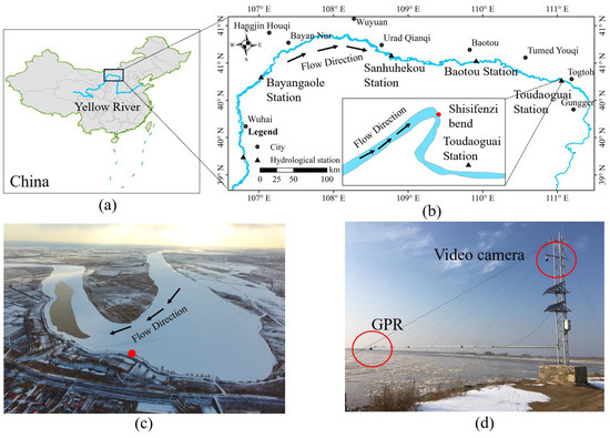
Figure 1.
(a) Yellow River mainstream, China; (b) Inner Mongolia reach of the Yellow River; (c) Shisifenzi bend of the Yellow River captured by UAV on 1 March 2022; (d) ice monitoring device mainly including video camera and ground penetrating radar (GPR) on the field. The video camera view is set to face the downstream of this bend. In (b,c), the red dot represents the location of ice monitoring device. The black triangle represents the location of hydrological station.
The ice monitoring device (Figure 1d) is located in the concave bank of Shisifenzi bend. Li et al. [47] introduces this device in detail, which includes mainly a video camera and a ground generating radar (GPR). The video camera, with infrared function, faces the downstream of this bend and automatically takes a 30 s video every hour to record drift ice on the bend during the freezing period and thawing period. The GPR could automatically and simultaneously measure ice thickness and water level each hour. Figure 2 shows a typical video image in which the near view is the concave bank and the far view is the convex bank.
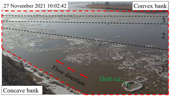
Figure 2.
A typical video image on 27 November 2021. The red dotted box is the area where the ice concentration is calculated. The black dotted line is the boundary for calculating ice drift velocity in zone 1, zone 2, and zone 3, which is from the concave bank to the convex bank.
2.2. Image Acquisition
During the freezing period in the winter of 2021–2022, the video camera first captured drift ice at 0:00 on 22 November 2021, when the air temperature was −8 °C. By 9:00 on 18 December 2021, the drift ice was not moving, and this bend was completely frozen-up. A total of 27 days of video images including drift ice were obtained, with a 30 s video every hour (at the beginning of the hour).
During the thawing period, due to the increase in air temperature, there was meltwater formation on the surface of the ice cover at the boundary of the concave bank on 11 March 2022. The ice cover of the main channel was broken up and drift ice flowed downstream on 13 March 2022. By 19:00 on 17 March 2022, there was no drift ice on the bend of the water surface. A total of 7 days of video images including drift ice were obtained, with a 30 s video per hour (at the beginning of the hour).
Although the video camera has infrared capability, it could only capture drift ice within a range of 50 m of the camera at night and did not cover the full view of the bend. Therefore, the images taken at night were not used to calculate ice concentration of the bend. These images could be used to calculate drift ice size, shape, and drift velocity near the concave bank.
3. Oblique Image Orthorectification Method and Calculation of Drift Ice Parameters
3.1. Basics of Photographic Images
Figure 3 shows a schematic diagram of the image coordinate system conversion method. The , are the camera point, the pixel point of image, and the true point on the ground, respectively. These three points are on a straight line. Equation (1) shows that the coordinate of point transfers from the image plane space to the ground plane space. Equation (2) is the transformation matrix () in Equation (1). Because are on a straight line, . Equation (3) shows the relationship between point and ground point . We bring Equation (3) into Equation (1) and eliminate the coefficient , getting Equation (4). Equation (4) shows another expression of the relationship between pixel point and ground point .
where from Equation (1) to Equation (2), ( is the coordinate of point in the image; is the distance from camera point to image center; ( is the coordinate of point in the ground; is the transformation matrix; is the tilt angle of the image; is the rotation angle of the image.
where from Equation (3) to Equation (4), ( is the coordinate of ground point ; is the distance from camera to ground point A in Figure 3; the other symbols are the same as in Equations (1) and (2).
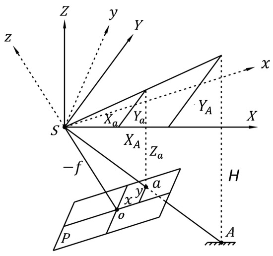
Figure 3.
Image coordinate system conversion. is the camera point; is the pixel point of image; is the true point on the ground; is the image plane; is the distance from camera point to image center; is the image center point; is the image coordinate system; is the ground coordinate system; ( is the coordinate of point in the image; ( is the coordinate of point in the ground; is the distance from camera to ground point A; ( is the coordinate of point in the ground.
3.2. Pixel Point Scale Method
In order to obtain the true size of the drift ice, this paper uses the pixel point scale method for orthorectification of the images. Equation (5) is this method expression, i.e., the ratio () of the length of the infinitesimal line ( in the image to the length of the corresponding ground line (. The infinitesimal line and corresponding ground line can be projected into the x and y directions, as shown in Equation (6) and Figure 4.
where from Equation (5) to Equation (6), is the scale from image to ground; is the length of the certain line in the image; is the length of the certain line in the corresponding ground; is the length of the infinitesimal line in the image; is the length of the infinitesimal line in the corresponding ground; and are the components of on the -axis and -axis; and are the components of on the -axis and -axis.
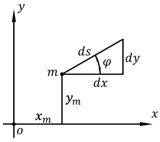
Figure 4.
The schematic diagram of the pixel point scale. is a pixel point; () is the coordinate of point ; is the angle between and axis.
To convert and to and , respectively, we bring Equation (4) into Equation (7). The conversion calculation process is given from Equations (8)–(11). Equation (11) is brought into Equation (6), getting Equation (12). Next, Equation (12) is brought into Equation (5), getting the pixel point scale without , as shown in Equation (13). Figure 4 shows the relationship between , and , as shown in Equation (14). Equations (14) and (15) are brought into Equation (13), getting the final pixel point scale () without and , as shown in Equation (16).
where from Equation (7) to Equation (16), are the hypothesized bridge variable; the other symbols are the same as in Equation (2) and Equation (4).
In Equation (16), there is the tilt angle (, the rotation angle (), direction angle (, the distance from camera to image center (, the distance from camera to ice surface (), and the image coordinate (,). Since the parameters () could not be obtained accurately, Equation (16) is simplified to Equation (17). In Equation (17), the parameters () need to be fitted through in-site calibration:
where is the pixel scale; is the distance from camera and ice surface; represent the horizontal and vertical pixel positions in the image, respectively. are the parameters that need to be fitted.
3.3. In-Site Calibration and Parameters Fitting
On 1 January 2022, we carried out in-situ calibrations on the stable ice cover. Two researchers walked on the ice cover with a 10 m length ( of rope tied around their waists, both keeping the rope always pulled tight. The third researcher directed them to walk from near view (concave bank) to far view (convex bank) by remote video, in case they walk out of video view.
Figure 5 shows all valid walking paths superimposed on one image, in which the 40 red lines represent the horizontal direction and the 21 blue lines represent non-horizontal direction. In addition, the ice surface altitude on this day was 989.02 m and the camera altitude was 1000.81 m, so the relative height between the ice surface and camera was 11.79 m.
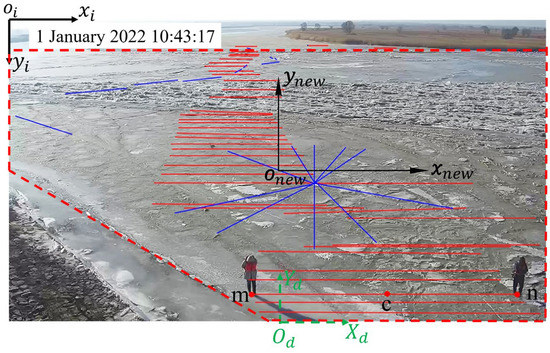
Figure 5.
In-situ calibrations [48]. The 40 red lines represent walk paths in the horizontal direction and the 21 blue lines represent the non-horizontal direction. The true distance of each line is 10 m. and represent the position of two researchers in the image. represents the midpoint of line . represents the default coordinate origin of the image. represents the center of the image. The green coordinate system is used to the corrected image display. is the midpoint of the lower edge of the image. The red dotted box is the sampling area where the drift ice is chosen to calculate ice size and shape.
In general, the upper left corner of the image is the default coordinate origin, as shown in in Figure 5. To apply the corrected method, the pixel coordinate origin of the image needs to be converted to the center of the image, to the right in the -positive direction and to the up in the -positive direction, as shown in Figure 5 for the coordinate system. The pixel coordinates of , , are extracted based on the new coordinate system. Because all images have a resolution of 72 dpi (pixels per inch), the side length () of each pixel is 3.528 × 10⁻⁴ m (Equation (18)); namely there are 2.8 pixels per millimeter. The pixel distance of Line (Figure 5) is calculated by Equation (19).
where is the side length of each pixel; is the absolute value of pixel distance of Line in Figure 5; and are the horizontal coordinates of point and point , respectively.
The ratio of the pixel distance to the true distance 10 m is approximated as the pixel scale of midpoint of the Line . In other words, Equation (20) is the expression of the above calculation when brought into Equation (17). The 40 red horizontal lines are first used to fit the -direction scale . The 21 non-horizontal lines are processed as the -direction line according to the Pythagorean theorem for triangles. After that, they are used to fit the y direction scale . Since the vertical distance between ice surface and camera varies with water level and the camera altitude is constant of 1000.81 m, the ice surface altitude is introduced, as shown in Equation (21). Equations (22) and (23) are the fitted results of the and directions, respectively.
Data for with an interval of 1 h can be obtained from the GPR [40] hanging over the river, as shown in Figure 1d. However, the waves in the river and the altitude difference between the ice top and the water surface were not considered. In the future, we will install a vertical video to monitor whether there is drift ice or water under the GPR when it is detecting. Moreover, we will do a continuous detection not hourly to find the altitude difference between the ice top and the water surface.
where is the pixel distance of Line in Figure 5; is the pixel scale of point c; and are the horizontal and vertical coordinates of point . is the vertical distance between ice surface and the camera; and are the pixel scale of horizontal and vertical position, respectively; is the ice or water surface altitude which is from GPR in the Figure 1d.
3.4. Image Correction Steps
In practical application, the oblique image becomes the orthographic image, requiring the following steps.
- Drift ice segmentation. Initially, we automatically used the thresholding method to segment drift ice in the original image (Figure 6a). However, some drift ice cannot be segmented because their grey is similar to the grey of water due to light at different time and drift ice thickness. The thinner drift ice is similar in grey to the water. In order to segment completely drift ice, we use Photoshop software (version: CS5) to draw all the drift ice marked in red, as shown in Figure 6b.
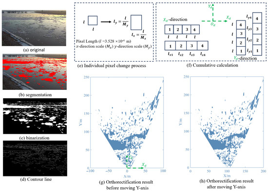 Figure 6. (a) original image; (b) segmentation image; (c) binarization image; (d) contour line; (e) diagram of the individual pixel correction process; (f) diagram of cumulative calculation; (g) orthorectified result before moving Y-axis; (h) orthorectified result after moving Y-axis. In (e), l is pixel length of 3.528 × 10⁻⁴ m in this paper. Mx and My represent the pixel scale in the x and y directions, respectively. x and y represent pixel position in the image. In (f), lx1, lx2, lx3, lx4 are the true length for pixel 1, 2, 3, 4, respectively, in Xd-direction; ly1, ly2, ly3, ly4 are the true length for pixel 1, 2, 3, 4, respectively, in Yd-direction; the green Xd-Yd coordinate system is used to the corrected image display, which is same as (g) and Figure 5.
 - Image binarization. Based on the red drift ice, we use the global threshold method in MATLAB software (version: R2021a) to convert images to binarization, as shown in Figure 6c.
- Based on the binarization image, the pixel coordinates of the contour line of each drift ice are extracted based on the binarization image, as shown in Figure 6d.
- These pixel coordinates are converted to the new coordinate system where the coordinate origin is the center of image (Figure 5). The original image is 1280 pixels wide and 720 pixels high. The side length () of each pixel is 3.528 × 10⁻⁴ m. Equation (24) is the conversion method for the new coordinate system.where ) is the default original coordinate; ) is the transformed coordinate, as shown in Figure 5.
- The calculation of the pixel point scale and . Each is brought into Equations (22) and (23) to calculate the pixel scale and in the direction and direction, respectively.
- The true length of individual pixels need be calculated by Equation (25), as shown in Figure 6e.where is the true length after correction in the -direction; is the true length after correction in -direction; is individual pixel length; and are the pixel scale.
- Orthorectification result. Figure 6g shows the orthorectification result of cumulation calculation. In order to avoid negative value, the Y-axis is moved to the left edge of the image, i.e., all pixels are added by 100 m in X-axis, as shown in Figure 6h. The final orthorectification image is shown in Figure 6h.
3.5. Calculation of Drift Ice Parameters
After oblique image correction, the true drift ice parameters (ice size, shape, movement) can be calculated. The size parameters include area (), perimeter (), equivalent diameter (). The shape parameters include roundness () and fractal dimension (). The motion parameters include ice concentration () and drift velocity (). These parameters are calculated as follows.
- Area (). In order to accurately calculate the parameter of individual drift ice, the separate and well-defined drift ice are manually selected and painted red in the Photoshop software. After image orthorectification, each drift ice is segmented and numbered, and the area is calculated in the Image J software (version: 1.1), which is also used to automatically calculate , , , and .
- Perimeter (). Counting the length of the pixel paths around the edge of drift ice.
- Equivalent diameter (). This equivalent diameter is known as the average Ferret diameter or average caliper diameter. Rothrock and Thorndike [49] and Lu et al. [50] introduced the measurements, namely measuring the distance between two parallel lines that are set against the drift ice’s sidewall. It can be directly calculated in the Image J software.
- Roundness (). Equation (26) is its calculation formula. When = 1, drift ice is circular. The closer is to 1, the more circular the drift ice.
- Fractal dimension (). Since pieces of drift ice can collide with each other, the fractal dimension is used to characterize the complexity and roughness of drift ice. This paper used the box-counting method [51,52] to calculate fractal dimension. It can be directly calculated in the Image J software. The larger the , the more curved the drift ice boundary [53].
- Drift velocity (). The video image is screenshotted every 5 s. The easily identifiable feature point of drift ice is selected, and its pixel coordinate is recorded and converted to the true position by Equations (22) and (23). In the image 5 s later, the pixel coordinate of the same feature points of the same drift ice is recorded and converted to the true position. The velocity is the ratio of the distance between the two true positions to 5 s. According to the division of the black dotted line in Figure 2, ice drift velocity of zone 1, zone 2, and zone 3 are calculated from the concave bank to the convex bank. Zone 1 is less than 30 m from the concave bank. Zone 2 is greater than 30 m and less than 80 m from the concave bank. Zone 3 is greater than 80 m and less than 120 m from the concave bank.
4. Results and Discussions
4.1. Calibration Accuracy Analysis
In-site calibration, we measure 61 data including 40 horizontal lines and 21 non-horizontal lines. The true length () of each line is 10 m. Based on corrected method, these lines of the oblique image is calculated to the actual length (. Their absolute error is calculated by Equation (27).
Figure 7a shows the 61 absolute error values range from 0.009 m to 0.850 m, with the average value of 0.236 m. The error is mainly distributed in 0–0.30 m with a total share of 69% (23% + 25% + 21%), as shown in Figure 7b.
where is the absolute error; is the calculated length based on the corrected method; is the true length of 10 m in-site calibration.
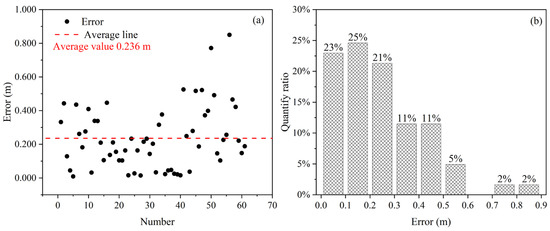
Figure 7.
(a) absolute error value for 61 data in-site calibration; (b) error distribution.
4.2. Drift Ice Size (Area, Perimeter, and Equivalent Diameter)
In the winter of 2021–2022, we chose 5–15 independent and well-defined drift ices in each hourly image. During the freezing period, we chose a total of 1527 drift ices. During the thawing period, we chose a total of 253 drift ices. These drift ices have been corrected to true size, as shown in Table 1.

Table 1.
The characteristic values of drift ice during the freezing and thawing period for area, perimeter, and equivalent diameter.
During the freezing period, the average area, perimeter, and equivalent diameter of drift ice are 6.50 m2, 10.00 m, and 3.36 m, respectively. During the thawing period, the average area, perimeter, and equivalent diameter of drift ice are 3.53 m2, 6.43 m, and 2.30 m, respectively. The values of parameters during the freezing period are greater than those during the thawing period. Table 1 also shows the range of observed values at the different period.
The area, perimeter and equivalent diameter are counted with quantify ratio at 1 m2, 5 m and 1 m intervals, respectively, as shown in Figure 8. Moreover, these distributions are fitted to the Gaussian function (Equation (28)), with the confidence of 95%. All fits are performed with the Origin software (version: 2023b). These fitted functions can be used as input parameters to the river ice process model in the future [14]. The fitted results are as shown in Table 2.
where is the drift ice size; is the quantity ratio of distribution. are the coefficients that need to be fitted.
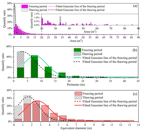
Figure 8.
Quantify ratio distribution of (a) area, (b) perimeter, and (c) equivalent diameter of drift ice during the freezing and thawing period.
Table 2.
The fitted result of Gaussian function of area, perimeter, and equivalent diameter.
Figure 8 shows the quantify ratio distribution of area, perimeter, and equivalent diameter of drift ice at the different period. During the freezing period, the drift ice area distribution ranges from 0 m2 to 90 m2 and is mainly in the range of 0–0.5 m2 and covers 41.5%. During the thawing period, the drift ice area distribution ranges from 0 m2 to 60 m2 and is mainly in the range of 0.5–1.0 m2 and covers 16.20% (Figure 5a). The larger drift ice (≥35 m2) is less than 1.9%. The perimeter distribution of the freezing period ranges from 0m to 45 m and is mainly in the range of 5–10 m and covers 42.93%. However, during the thawing period, the perimeter distribution ranges from 0 m to 35 m and is mainly in the range of 0–5 m and covers 50.20% (Figure 8b). During the freezing period, the equivalent diameter distribution ranges from 0 m to 14 m and is mainly in the range of 2–3 m (25.79%). During the thawing period, it ranges from 0 m to 13 m and is mainly in the range of 1–2 m (33.60%) during the thawing period (Figure 8c).
This paper focuses on the analysis of drift ice size characteristics and variability as a proxy for equivalent diameter. As shown in Table 2, the mathematical expectation () of the equivalent diameter for the freezing period is focused toward 2.656 m, while the expectation () is 1.611 m for the thawing period. Their mathematical standard deviations () are not very different, being 2.677 and 2.408, respectively. The above analysis shows that drift ice size is larger during the freezing period than during the thawing period. This is because more frazil ice is gathering toward drift ice when it moves downstream, making it larger. However, during the thawing period, drift ice is of low strength and becomes smaller when pieces of drift ice collide with each other as they move downstream.
Figure 9a shows the drift ice size (equivalent diameter) is on an increasing trend during the freezing period. This may be related to negative air temperature. The lower the air temperature, the earlier frazil ice is produced and the larger the accumulation. Figure 9b shows the drift ice size is on a decreasing trend during the thawing period. This may be related to the distance of drift ice movement. Ice blocks are initially large when they break up but become smaller as the distance travelled increases and they collide with the embankment or with each other.
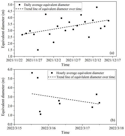
Figure 9.
Equivalent diameter over time during the (a) freezing period and (b) thawing period.
4.3. Drift Ice Shape (Fractal Dimension and Roundness)
Table 3 shows the average value and the range of observed values for the fractal dimension and roundness. For the fractal dimension, the range of observations is from 1.000 to 1.298, with a mean value of 1.107 during the freezing period. During the thawing period, the range of observations is from 1.001 to 1.295, with a mean value of 1.110. For the roundness, the range of observations is from 0.179 to 0.946, with a mean value of 0.660 during the freezing period. During the thawing period, the range of observations is from 0.263 to 0.988, with a mean value of 0.697.
Table 3.
The characteristic values of drift ice during freezing and thawing period for the fractal dimension and roundness.
The fractal dimension and roundness are counted with the quantify ratio at 0.02 and 0.1 intervals, respectively, as shown in Figure 10. Moreover, these distributions are fitted to Gaussian function (Equation (28)), with the confidence of 95%. All fits are performed with the Origin software. These fitted functions can also be used to as input parameters to the river ice process model in the future [14]. The fitted results are as shown in Table 4.
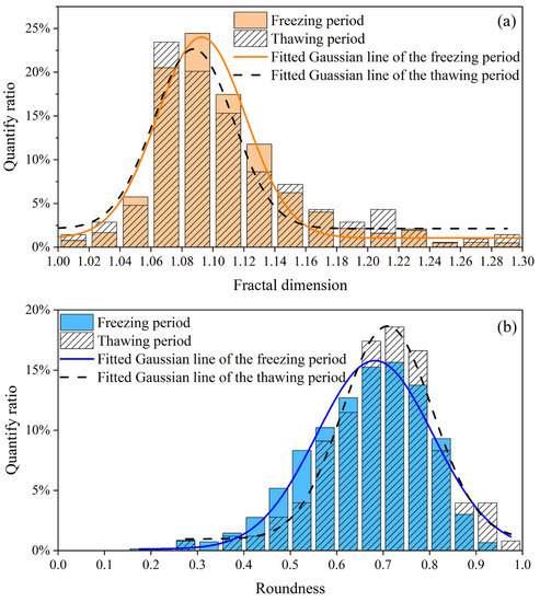
Figure 10.
Quantify ratio distribution of the (a) fractal dimension and (b) roundness of drift ice at the different period.
Table 4.
The fitted result of Gaussian function of the fractal dimension and roundness.
Figure 10a shows the fractal dimension of drift ice is mainly distributed in the range of 1.0–1.3, with the highest quantify ratio of 24.45% at 1.08–1.10 during the freezing period and 23.44% at 1.06–1.08 during the thawing period. As shown in Table 4, the mathematical expectation () of the fractal dimension is 1.093, which is slightly higher than that for the thawing period, which is 1.087. Their mathematical standard deviations () are in the same order of magnitude, being 0.057 and 0.051, respectively, indicating that they have the same degree of dispersion at the distribution of fractal dimension.
Figure 10b shows the roundness of drift ice is mainly distributed in the range of 0.1–1.0, with the maximum quantify ratio of 15.64% at 0.70–0.75 during the freezing period and 18.58% at 0.70–0.75 during the thawing period. Table 2 shows the Gaussian distribution fit for the roundness also has a high goodness fit, with = 0.956 and = 0.969 for the freezing period and thawing period, respectively. The mathematical expectation () of 0.682 for roundness during the freezing period is less than that of 0.709 during the thawing period, indicating that drift ice during the thawing period is closer to circular. The mathematical standard deviation () of 0.251 during the freezing period is larger than that of 0.193 during the thawing period, indicating the distribution of roundness during the freezing period is more dispersed.
During the freezing period, the fractal dimension and roundness of the daily average are calculated and plotted in Figure 11a. Since the thawing period is short, the fractal dimension and roundness hourly average are calculated and plotted in Figure 11b. Figure 11a shows the fractal dimension is on the increasing trend and the roundness is on the decreasing trend, indicating the drift ice edge is becoming more complex and less rounded. During the thawing period, as shown in Figure 11b, the trend of fractal dimension and roundness is opposite to that of the freezing period. The drift ice is becoming more rounded. Because judging from the ice cover cracks, initially broken drift ice is similar to a square, and the drift ice gradually tends to round as the ice blocks move and rub against each other.
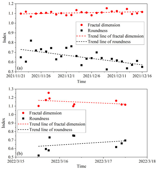
Figure 11.
The average fractal dimension and roundness over time during the (a) freezing period and (b) thawing period.
4.4. Ice Concentration and Drift Velocity
After the image orthorectification, the process of the ice concentration and drift velocity during the freezing period and thawing period are plotted in Figure 12 and Figure 13. Meanwhile, we also collect the air temperature at the same time.
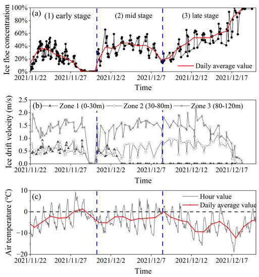
Figure 12.
Time variation of the (a) ice concentration, (b) ice drift velocity, and (c) air temperature during the freezing period. In (b), zone 1, zone 2, and zone 3 are located from the concave bank to the convex bank in the Shisifenzi bend, as shown in Figure 2.
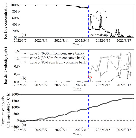
Figure 13.
Time variation of the (a) ice concentration, (b) ice drift velocity, and (c) cumulative hourly positive air temperature during the thawing period. In (b), zone 1, zone 2, and zone 3 are located from the concave bank to the convex bank in the Shisifenzi bend, as shown in Figure 2. The red and black dotted circle represent surge points.
Analyzing the relationship between air temperature and ice concentration is important for the forecasting of river ice conditions during the freezing and thawing processes. Changes in the ice concentration determine when the river is freezing and thawing. In the future, changes in river freezing and thawing could be predicted by the air temperature, so that the flow released from upstream dams can be adjusted in time to avoid ice flooding. In addition, understanding the relationship between ice concentration and drift velocity should not be neglected. In general, ice drift velocity is affected by hydrodynamic conditions, e.g., discharge, water, speed, and slope. This knowledge can lead to a lack of ice concentration considerations when modelling ice drift velocity, especially at a high ice concentration.
Figure 12a shows that the change of ice concentration has gone through three stages (early stage, mid stage and late stage) from 22 November 2021 to 18 December 2021. In the early stage, the ice concentration firstly increases to around 50% and then decreases to 0 (not drift ice). In this stage, the air temperature (Figure 12c) is rising, reaching the highest temperature of 9.3 °C at 15:00 on 27 November 2021. This may be because the higher the air temperature, the less frazil ice is produced and the lower the ice concentration. Moreover, as shown in Figure 12b, the ice drift velocity of zone 1 and zone 2 fluctuates in the range of 0.38–0.92 m/s. The drift velocity of zone 3 fluctuates in the range of 1.01–1.96 m/s, which is greater than that of zone 1 and zone 2. This is because zones 1 and 2 are areas of slow flow in the concave bank.
In the mid stage, as air temperature drops to −9.9 °C at 5:00 on 1 December 2021, the ice concentration rises rapidly to around 65.8%. After that, the ice concentration remains at around 40.3% when the daily average air temperature remains at around −2.9 °C. At the end of this stage, the ice concentration drops rapidly to 17.8% as the average air temperature increases to 0 °C. Furthermore, the ice drift velocity of zone 1 drops to 0 m/s at 7:00 on 3 December 2021, since the drift ice of zone 1 has fully frozen to form fixed shore ice.
In the late stage, from 8 December 2021 to 18 December 2021, the ice concentration rises from 17.8% to 100%. This is because the air temperature is continuing to fall, with the lowest of −18.5 °C at 7:00 on 17 December 2021. In addition, on 16 December 2021, the ice drift velocity drops rapidly, indicating the formation of ice jam at the bend.
Figure 13a shows the variation of ice concentration during the thawing period. Before ice cover breaks up, the ice concentration is slowly decreasing from 11 March 2022. This is due to the melting of the ice cover surface closer to the concave bank, which the images show as water. At 14:00 on 14 March 2022, the ice concentration reduced to 27.2% very quickly, because ice cover in zone 3 (mainstream region) suddenly breaks up and flowed downstream. This is because the cumulative positive air temperature causes the ice temperature to increase, the ice strength to decrease and ice cover breaks up. At this time, the cumulation hourly positive air temperature reaches 920.4 °C·h (Figure 13c).
After ice cover breaks up, the ice concentration gradually decreases, but has two high values, as shown in the black dotted circle of Figure 13a. This is because ice cover upstream also breaks up and a large number of drift ice suddenly entered this bend.
Figure 13b shows the variation of ice drift velocity at the different zone. The drift ice of zone 3 move first, followed by zone 2 and finally zone 1, because zone 3 is the mainstream region. As shown in the red dotted circle in Figure 13b, there is a high velocity value in zone 2. This is because the ice cover slides under the dragging force of the water, but without breaking up.
Figure 14 shows the relationship between ice concentration and drift velocity. During the freezing period (Figure 14a), when the ice concentration is less than 40%, the ice drift velocity fluctuates in the range of 0.55–1.11 m/s. When the ice concentration is larger than 40% and less than 90%, the ice drift velocity drops rapidly. When it is greater than 90%, the ice drift velocity levels off to near 0.05 m/s. This is because at a low ice concentration pieces of drift ice are relatively independent and do not interact with each other. However, when the ice concentration increases to a certain level, pieces of drift ice will collide with each other and pile up, making the ice drift velocity slow down. It is inappropriate to use ice drift velocity as a proxy for water surface velocity to measure discharge when the ice concentration is greater than 40%.
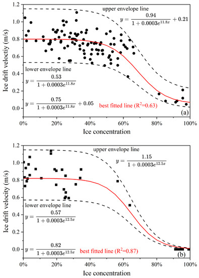
Figure 14.
The relationship between ice concentration and drift velocity during the (a) freezing period and (b) thawing period.
During the thawing period (Figure 14b), the change between ice concentration and drift velocity is similar to the change during the freezing period. The difference is that when ice concentration is less than 40%, ice drift velocity fluctuates in the range of 0.59–1.14 m/s. Moreover, when it is larger than 90%, ice drift velocity is 0 m/s. This is because the ice cover near the bank melts first, but the ice cover does not break up and move.
The Logistic function (Equation (29)) is used to fit the relationship between ice concentration and ice drift velocity. We give not only the best fitted line but also the upper envelop line and the lower envelop line. Table 5 gives the fitted parameters.
where represents ice concentration; represents ice drift velocity; need to be fitted.
Table 5.
Logistic function parameters for the relationship between ice concentration and drift velocity.
For the above analyses, we have briefly analysed the effect of air temperature on changes in the ice concentration process during the freezing and thawing period. However, these ice parameters’ change processes would be influenced by a variety of factors such as air temperature, water temperature, temperature gradient, wind speed and direction, solar radiation, discharge, water level, current speed, etc.
In addition, the statistics and estimates of the ice parameters may be different from year to year. It is necessary to accumulate ice parameters from many winter seasons and collect all the meteorological and hydrological data at the same time. In the future, by statistically analysing data from many years of winters, we will attempt to establish patterns of the freezing and thawing of river ice.
5. Conclusions
This study introduces a survey method of drift ice in the Yellow River, China. In the winter of 2021–2022, shore-based oblique hourly images are acquired during the freezing and thawing periods. Because the images are oblique, the image scale is different from near view to far view. To obtain the true size of drift ice, the pixel point scale method is presented which gives the scale of each pixel position of the oblique image. By using in-situ calibration on the stable ice cover, the unknown parameters of pixel point scale equation are fitted. Based on the corrected method, the length of 61 measured lines were compared with the corresponding calculated length to obtain the absolute error. The absolute error ranges from 0.009 m to 0.850 m, with the average value of 0.236 m. In comparison with UAV and satellite remote sensing monitoring, this survey method allows for continuous drift ice parameters. Compared to staff monitoring, this survey method increases accuracy for the true drift ice parameters. The method can also be extended to other rivers or lakes in cold regions.
After the correction of oblique images, the true drift ice parameters, e.g., ice area, perimeter, equivalent diameter, fractal dimension, roundness, concentration, and drift velocity, can be obtained. In the winter of 2021–2022, the observed drift ice area ranges from 0.11 m2 to 85.60 m2, with a mean value of 6.50 m2 during the freezing period. When it is the thawing period, the drift ice area ranges from 0.02 m2 to 55.22 m2, with a mean value of 3.53 m2. The observed drift ice perimeter ranges from 1.32 m to 46.18 m, with a mean value of 10.00 m during the freezing period. When it is the thawing period, the drift ice perimeter ranges from 0.48 m to 32.12 m, with a mean value of 6.43 m. The observed drift ice equivalent diameter ranges from 0.52 m to 13.10 m, with a mean value of 3.36 m during the freezing period. When it is the thawing period, the drift ice equivalent diameter ranges from 0.20 m to 12.54 m, with a mean value of 2.30 m. Compared with the above data, the average size of the drift ice during the freezing period is larger than that during the thawing period. Plotting their time series data, the drift ice size increases during the freezing period; however, it is decreasing during the thawing period.
For the fractal dimension and roundness, the observed drift ice fractal dimension is in the range of 1.000–1.298, with a mean value of 1.107 during the freezing period. When it is the thawing period, the fractal dimension is in the range of 1.001–1.295, with a mean value of 1.110. The observed drift ice roundness is in the range of 0.179–0.946, with a mean value of 0.660 during the freezing period. When it is the thawing period, the roundness is in the range of 0.263–0.988, with a mean value of 0.697. Plotting their time series data, during the freezing period, the fractal dimension is increasing, and the roundness is decreasing, indicating the drift ice is becoming less rounded. However, during the thawing period, the fractal dimension is decreasing, and the roundness is increasing, indicating the drift ice is becoming more rounded.
In addition, the distributions of ice area, perimeter, equivalent diameter, fractal dimension and roundness are estimated using the Gaussian function with the confidence of 95%. These distributions can be used as a boundary condition for the river ice process model in the future.
The time series of the corrected ice concentration and drift velocity are also obtained. By observing the variation of ice drift velocity of zone 1, zone 2, and zone 3, the sequence of the freezing and thawing of the river bend is obtained, which is from the concave bank to the convex bank during the freezing, and during the thawing period it is reversed. There is a non-linear relationship between ice concentration and drift velocity. The inflection point exists at 40% and 90% for the ice concentration. The relationship between ice concentration and drift velocity is potentially expressed as a Logistic function.
Author Contributions
Conceptualization, C.L.; methodology, C.L. and Z.L.; validation, H.Z., S.W., B.Z. and Y.D.; formal analysis, C.L., H.Z. and S.W.; investigation, C.L.; resources, B.Z. and Y.D.; data curation, B.Z.; writing—original draft preparation, C.L.; writing—review and editing, Z.L., C.L., H.Z., S.W. and Y.D.; visualization, C.L.; project administration, Z.L. and Y.D.; funding acquisition, Y.D. and Z.L. All authors have read and agreed to the published version of the manuscript.
Funding
This research was funded by the National Natural Science Foundation of China (51979024), the Special Funds for Basic Scientific Research of the Yellow River Institute of Hydraulic Research (HKY-JBYW-2022-08).
Data Availability Statement
Not applicable.
Conflicts of Interest
The authors declare no conflict of interest. The funders had no role in the design of the study; in the collection, analyses, or interpretation of data; in the writing of the manuscript; or in the decision to publish the results.
References
- Chu, T.; Lindenschmidt, K. Integration of space-borne and air-borne data in monitoring river ice processes in the Slave River, Canada. Remote Sens. Environ. 2016, 181, 65–81. [Google Scholar] [CrossRef]
- McFarlane, V.; Loewen, M.; Hicks, F. Field measurements of suspended frazil ice—Part II: Observations and analyses of frazil ice properties during the principal and residual supercooling phases. Cold Reg. Sci. Technol. 2019, 165, 102796. [Google Scholar] [CrossRef]
- Zhang, Y.; Li, Z.; Xiu, Y.; Li, C.; Zhang, B.; Deng, Y. Microstructural characteristics of frazil particles and the physical properties of frazil ice in the Yellow River, China. Crystals 2021, 11, 617. [Google Scholar] [CrossRef]
- Kempema, E.W.; Ettema, R. Anchor ice rafting: Observations from the Laramie River. River Res. Appl. 2011, 27, 1126–1135. [Google Scholar] [CrossRef]
- Beltaos, S. Threshold between mechanical and thermal breakup of river ice cover. Cold Reg. Sci. Technol. 2003, 37, 1–13. [Google Scholar] [CrossRef]
- Ashton, G.D. River ice. Annu. Rev. Fluid Mech. 1978, 10, 369–392. [Google Scholar] [CrossRef]
- Liu, L.; Li, H.; Shen, H. A two-dimensional comprehensive river ice model. In Proceeding of the 18th IAHR International Symposium on Ice, Sapporo, Japan, 28 August–1 September 2006. [Google Scholar]
- Shen, H.T. Mathematical modeling of river ice processes. Cold Reg. Sci. Technol. 2010, 62, 3–13. [Google Scholar] [CrossRef]
- Lindenschmidt, K. RIVICE-A non-proprietary, open-source, one-dimensional river-ice model. Water 2017, 9, 314. [Google Scholar] [CrossRef]
- Knack, I.M.; Shen, H.T. Numerical modeling of ice transport in channels with river restoration structures. Can. J. Civ. Eng. 2017, 44, 813–819. [Google Scholar] [CrossRef]
- Zhai, B.; Liu, L.; Shen, H.T.; Ji, S. A numerical model for river ice dynamics based on discrete element method. J. Hydraul. Res. 2022, 60, 543–556. [Google Scholar] [CrossRef]
- Blackburn, J.; She, Y. A comprehensive public-domain river ice process model and its application to a complex natural river. Cold Reg. Sci. Technol. 2019, 163, 44–58. [Google Scholar] [CrossRef]
- Chassiot, L.; Lajeunesse, P.; Bernier, J. Riverbank erosion in cold environments: Review and outlook. Earth-Sci. Rev. 2020, 207, 103231. [Google Scholar] [CrossRef]
- Vandermause, R.; Harvey, M.; Zevenbergen, L.; Ettema, R. River-ice effects on bank erosion along the middle segment of the Susitna river, Alaska. Cold Reg. Sci. Technol. 2021, 185, 103239. [Google Scholar] [CrossRef]
- Ettema, R.; Zabilansky, L. Ice influences on channel stability: Insights from Missouri’s Fort Peck reach. J. Hydraul. Eng. 2004, 130, 279–292. [Google Scholar] [CrossRef]
- Beltaos, S.; Burrell, B.C. Transport of suspended sediment during the breakup of the ice cover, Saint John River, Canada. Cold Reg. Sci. Technol. 2016, 129, 1–13. [Google Scholar] [CrossRef]
- Kalke, H.; Loewen, M. Support vector machine learning applied to digital images of river ice conditions. Cold Reg. Sci. Technol. 2018, 155, 225–236. [Google Scholar] [CrossRef]
- Chen, P.; Cheng, T.; Wang, J.; Cao, G. Accumulation and evolution of ice jams influenced by different ice discharge: An experimental analysis. Front. Earth Sci. 2023, 10, 1054040. [Google Scholar] [CrossRef]
- Luo, H.; Ji, H.; Gao, G.; Zhang, B.; Mou, X. Study on the characteristics of flow and ice jam in Shisifenzi bend in the Yellow River during the freeze-up period. J. Hydraul. Eng. 2020, 51, 1089–1100. (In Chinese) [Google Scholar] [CrossRef]
- Fu, H.; Guo, X.; Wu, P.; Wang, T.; Guo, Y.; Li, J. River-ice blasting, and explosive weight optimization for ice-flooding mitigation: A case study. Cold Reg. Sci. Technol. 2020, 177, 103103. [Google Scholar] [CrossRef]
- Beltaos, S.; Bonsal, B. Climate change impacts on Peace River ice thickness and implications to ice-jam flooding of Peace-Athabasca Delta, Canada. Cold Reg. Sci. Technol. 2021, 186, 103279. [Google Scholar] [CrossRef]
- Beltaos, S. The role of waves in ice-jam flooding of the Peace—Athabasca Delta. Hydrol. Process. 2007, 21, 2548–2559. [Google Scholar] [CrossRef]
- Beltaos, S. Ice-jam flood regime of the Peace-Athabasca Delta: Update in light of the 2014 event. Cold Reg. Sci. Technol. 2019, 165, 102791. [Google Scholar] [CrossRef]
- Luo, D. Yellow River Ice Disaster Risk Management Based on Grey Prediction and Decision Method. In Emerging Studies and Applications of Grey Systems; Yang, Y., Liu, S., Eds.; Springer: Singapore, 2023; pp. 183–219. [Google Scholar] [CrossRef]
- Zakharova, E.; Agafonova, S.; Duguay, C.; Frolova, N.; Kouraev, A. River ice phenology and thickness from satellite altimetry: Potential for ice bridge road operation and climate studies. Cryosphere 2021, 15, 5387–5407. [Google Scholar] [CrossRef]
- Yang, Q.; Song, K.; Hao, X.; Wen, Z.; Tan, Y.; Li, W. Investigation of spatial and temporal variability of river ice phenology and thickness across Songhua River Basin, northeast China. Cryosphere 2020, 14, 3581–3593. [Google Scholar] [CrossRef]
- Rokaya, P.; Morales-Marín, L.; Bonsal, B.; Wheater, H.; Lindenschmidt, K. Climatic effects on ice phenology and ice-jam flooding of the Athabasca River in western Canada. Hydrol. Sci. J. 2019, 64, 1265–1278. [Google Scholar] [CrossRef]
- Liu, B.; Ji, H.; Zhai, Y.; Luo, H. Estimation of river ice thickness in the Shisifenzi reach of the Yellow River with remote sensing and air temperature data. IEEE J. Sel. Top. Appl. Earth Obs. Remote Sens. 2023, 16, 5645–5659. [Google Scholar] [CrossRef]
- Li, H.; Li, H.; Wang, J.; Hao, X. Monitoring high-altitude river ice distribution at the basin scale in the northeastern Tibetan Plateau from a Landsat time-series spanning 1999–2018. Remote Sens. Environ. 2020, 247, 111915. [Google Scholar] [CrossRef]
- Li, H.; Li, H.; Wang, J.; Hao, X. Revealing the river ice phenology on the Tibetan Plateau using Sentinel-2 and Landsat 8 overlapping orbit imagery. J. Hydrol. 2023, 619, 129285. [Google Scholar] [CrossRef]
- Zhang, F.; Mosaffa, M.; Chu, T.; Lindenschmidt, K.-E. Using remote sensing data to parameterize ice jam modeling for a northern inland delta. Water 2017, 9, 306. [Google Scholar] [CrossRef]
- Bourgault, D. Shore-based photogrammetry of river ice. Can. J. Civil Eng. 2008, 35, 80–86. [Google Scholar] [CrossRef][Green Version]
- Ansari, S.; Rennie, C.D.; Seidou, O.; Malenchak, J.; Zare, S.G. Automated monitoring of river ice processes using shore-based imagery. Cold Reg. Sci. Technol. 2017, 142, 1–16. [Google Scholar] [CrossRef]
- Deng, Y.; Li, C.; Li, Z.; Zhang, B. Dynamic and full-time acquisition technology and method of ice data of Yellow River. Sensors 2021, 22, 176. [Google Scholar] [CrossRef]
- Wang, E.; Hu, S.; Han, H.; Li, Y.; Ren, Z.; Du, S. Ice velocity in upstream of Heilongjiang Based on UAV low-altitude remote sensing and the SIFT algorithm. Water 2022, 14, 1957. [Google Scholar] [CrossRef]
- Das, A.; Sagin, J.; Sanden, J.; Evans, E.; Mckay, H.; Lindenschmidt, K. Monitoring the freeze-up and ice cover progression of the Slave River. Can. J. Civ. Eng. 2015, 42, 609–621. [Google Scholar] [CrossRef]
- Zhang, X.; Jin, J.; Lan, Z.; Li, C.; Fan, M.; Wang, Y.; Yu, X.; Zhang, Y. ICENET: A Semantic Segmentation Deep Network for River Ice by Fusing Positional and Channel-Wise Attentive Features. Remote Sens. 2020, 12, 221. [Google Scholar] [CrossRef]
- Zhang, X.; Zhou, Y.; Jin, J.; Wang, Y.; Fan, M.; Wang, N.; Zhang, Y. ICENETv2: A Fine-Grained River Ice Semantic Segmentation Network Based on UAV Images. Remote Sens. 2021, 13, 633. [Google Scholar] [CrossRef]
- Ansari, S.; Rennie, C.D.; Clark, S.P.; Seidou, O. IceMaskNet: River ice detection and characterization using deep learning algorithms applied to aerial photography. Cold Reg. Sci. Technol. 2021, 189, 103324. [Google Scholar] [CrossRef]
- Pei, C.; She, Y.; Loewen, M. Deep learning-based river surface ice quantification using a distant and oblique-viewed public camera. Cold Reg. Sci. Technol. 2023, 206, 103736. [Google Scholar] [CrossRef]
- Emond, J.; Morse, B.; Richard, M.; Stander, E.; Viau, A.A. Surface ice observations on the St. Lawrence River using infrared thermography. River Res. Appl. 2011, 27, 1090–1105. [Google Scholar] [CrossRef]
- Daigle, A.; Bérubé, F.; Bergeron, N.; Matte, P. A methodology based on Particle image velocimetry for river ice velocity measurement. Cold Reg. Sci. Technol. 2013, 89, 36–47. [Google Scholar] [CrossRef]
- Morse, B.; Hessami, M.; Bourel, C. Characteristics of ice in the St. Lawrence River. Can. J. Civ. Eng. 2003, 30, 766–774. [Google Scholar] [CrossRef]
- Ghobrial, T.R.; Loewen, M.R.; Hicks, F.E. Continuous monitoring of river surface ice during freeze-up using upward looking sonar. Cold Reg. Sci. Technol. 2013, 86, 69–85. [Google Scholar] [CrossRef]
- Li, C.; Li, Z.; Yang, Y.; Wang, Q.; Zhang, B.; Deng, Y. Theory and application of ice thermodynamic and mechanics for the natural sinking of gabion mattresses on a floating ice cover. Cold Reg. Sci. Technol. 2023, 213, 103925. [Google Scholar] [CrossRef]
- Li, C.; Li, Z.; Huang, W.; Zhang, B.; Deng, Y.; Li, G. Morphology dynamics of ice cover in a river bend revealed by the UAV-GPR and sentinel-2. Remote Sens. 2023, 15, 3180. [Google Scholar] [CrossRef]
- Li, Z.; Li, C.; Yang, Y.; Zhang, B.; Deng, Y.; Li, G. Physical Mechanism and Parameterization for Correcting Radar Wave Velocity in Yellow River Ice with Air Temperature and Ice Thickness. Remote Sens. 2023, 15, 1121. [Google Scholar] [CrossRef]
- Wu, S.; Li, C.; Li, Z.; Zhang, L.; Zhang, B.; Deng, Y. Theoretical basis, and practice of improving the accuracy of identifying river slope ice run image. Yellow River 2023, 45, 115–120,125. (In Chinese) [Google Scholar] [CrossRef]
- Rothrock, D.A.; Thorndike, A.S. Measuring the sea ice floe size distribution. J. Geophys. Res. Ocean. 1984, 89, 6477–6486. [Google Scholar] [CrossRef]
- Lu, P.; Li, Z.; Zhang, Z.; Dong, X. Aerial observations of floe size distribution in the marginal ice zone of summer Prydz Bay. J. Geophys. Res. Ocean. 2008, 113, C02011. [Google Scholar] [CrossRef]
- Weiss, J. Fracture and fragmentation of ice: A fractal analysis of scale invariance. Eng. Fract. Mech. 2001, 68, 1975–2012. [Google Scholar] [CrossRef]
- Ai, T.; Zhang, R.; Zhou, H.W.; Pei, J.L. Box-counting methods to directly estimate the fractal dimension of a rock surface. Appl. Surf. Sci. 2014, 314, 610–621. [Google Scholar] [CrossRef]
- Allen, M.; Brown, G.J.; Miles, N.J. Measurement of boundary fractal dimensions: Review of current techniques. Powder Technol. 1995, 84, 1–14. [Google Scholar] [CrossRef]
Disclaimer/Publisher’s Note: The statements, opinions and data contained in all publications are solely those of the individual author(s) and contributor(s) and not of MDPI and/or the editor(s). MDPI and/or the editor(s) disclaim responsibility for any injury to people or property resulting from any ideas, methods, instructions or products referred to in the content. |
© 2023 by the authors. Licensee MDPI, Basel, Switzerland. This article is an open access article distributed under the terms and conditions of the Creative Commons Attribution (CC BY) license (https://creativecommons.org/licenses/by/4.0/).