Drought Hazard Analysis in the Jilin Province Based on a Three-Dimensional Copula Method

Abstract

Based on the precipitation and potential evapotranspiration at 23 stations in the Jilin Province, the standardized precipitation evapotranspiration index (SPEI) was calculated. Based on run theory and combined with previous research in Jilin Province, we redefine the drought threshold, with three characteristics, that is, drought duration, intensity, and severity, were identified and extracted. Two- and three-dimensional copula functions were selected to fit and combine drought variables to calculate the joint recurrence period. In order to make the alternative copula model more complete, 25 representative copula functions are selected for the first time to construct the Joint probability distribution function. The Mann–Kendall test was used to examine abrupt changes in Meihekou County. SPEI trends and the joint cumulative probability of drought variables in the Changbai area were analyzed. The results show that: (1) the SPEI in the Meihekou area was unstable around 2000 and 2010, with abrupt change points; (2) the trend of the SPEI in the Changbai Mountains area indicates that the drought occurrence is similar at various timescales; the drought range and duration increase with increasing timescale; and (3) the correlation between the three drought variables is strong and the fit is good. The results of two- and three-dimensional joint recurrence period calculations are similar, with a high probability of recurrence within three years.

1. Introduction

Drought is one of the largest and most destructive natural disasters globally, accounting for 45% of all deaths since 1970. Ninety percent of deaths occur in developing countries. Drought has also become an important factor impeding China’s economic development because of national circumstances, the specificities of China’s geographical situation, and meteorological characteristics. Drought disasters have occurred in China over the past 20 years. Precipitation has been relatively low in most parts of northeastern China since the autumn of 2002, with 3–8% less rainfall than usual in both the winter and spring of 2003, especially from January–May 2003 when the average precipitation was even lower, marking the third year of low rainfall since 1954 [1]. Over the past 30 years, drought has been the main type of agricultural disaster in the Jilin Province and its development is generally consistent with the overall disaster trend, with droughts occurring in the western regions of Jilin, Baicheng, and Songyuan, and increasing in the mid-1990s in Changchun, Siping, and Tonghua in the east [2]. Droughts in the Jilin Province are characterized by a “wave” pattern of change, with an increase in the overall drought conditions and a gradual regional extension from the most drought-prone western plains to the central and eastern parts of the province. Agriculture in the Jilin Province faces serious challenges. To mitigate the effects of drought on local areas and facilitate the development of drought prevention and control measures and emergency plans by local authorities, the risk of drought occurrences in the Jilin Province must be analyzed [3].

Currently, many scholars are conducting drought research; however, most traditional drought studies are based on frequency characteristics to portray drought events. However, drought occurrence depends on various factors and single drought variables cannot objectively and comprehensively describe drought events. Therefore, most scholars utilize multivariate drought analysis. The main method that is currently used to construct multivariate joint distribution is the copula function method [4]. The copula function is a statistical tool used to study the dependence between multiple variables without focusing on their marginal distributions. It is widely used in the fields of climatology and environmental sciences, and is particularly suited to the study of extreme weather events such as droughts. By introducing the copula function, we are able to achieve more specific and accurate results in drought risk assessment. This will help to deepen the understanding of drought events and provide a more effective basis for decision-making in the areas of drought monitoring, water resource management, and climate change adaptation. For example, Yang et al. [5]. selected a standardized evapotranspiration index and analyzed the recurrence period of drought events in different regions using a two-dimensional copula function. Wang et al. [6]. extracted the frequency and intensity of drought events from a standardized precipitation index based on tour theory and used the copula function with the best fit to fit the drought characteristic variables to analyze the joint cumulative probability of drought characteristic variables and the joint recurrence period of drought events. Zhu et al. [7]. used the SPEI to identify drought events. They isolated three drought characteristic variables, that is, the drought ephemeris, drought intensity, and drought intensity peak, and selected two- and three-dimensional copula functions to fit and combine the drought characteristic variables to calculate the joint and concurrent recurrence periods. Biniyam et al. [8]. selected the best-fit copula function to construct a joint probability distribution (JPD) of the standardized precipitation index (SPI) and standardized soil moisture index (SSMI) to analyze meteorological drought in the upper reaches of the Tekeze River Basin in northern Ethiopia. In this study, we use the copula function to analyze the joint distribution of drought variables and risk assessment.

In this study, the Jilin Province was chosen as the study region [9]. The importance of using the Standardized Precipitation Evapotranspiration Index (SPEI) in drought analysis lies in its comprehensive consideration of both precipitation and evapotranspiration effects, thereby providing a more holistic reflection of drought conditions. Compared with single indices such as the Standardized Precipitation Index (SPI) or Evapotranspiration Index (ETI), SPEI incorporates the influence of temperature on water utilization, enabling a more accurate characterization of the water supply–demand balance and revealing the true occurrence and persistence of drought events.

The application of copula models in calculating drought recurrence periods enhances the precision and accuracy of drought analysis. By combining multiple drought variables through joint probability density functions and copula functions, this approach enables a better exploration of the interrelationships and dependencies among drought variables, leading to a more comprehensive assessment of drought risk. In contrast, traditional single index methods can only provide partial information on drought, failing to capture the complexity of drought events.

Through the use of SPEI and copula models, we can obtain joint probability distributions and recurrence periods of drought events, facilitating more precise estimations of the probabilities and return periods of various drought severities. This has significant implications for drought risk assessment, water resource management, and disaster preparedness, empowering decision-makers to formulate more effective strategies and measures to address drought challenges. Consequently, the application of SPEI and copula models enhances the reliability and practicality of drought analysis, contributing to a better understanding and mitigation of drought phenomena. Therefore, utilizing the monthly scale SPEI data from 1960 to 2012, we extracted three drought characteristic variables, namely drought intensity, duration, and severity, using the run theory method. Subsequently, we employed the copula approach to analyze the multidimensional joint distribution and recurrence periods of drought variables in Jilin Province.

2. Materials and Data

2.1. Overview of the Study Region

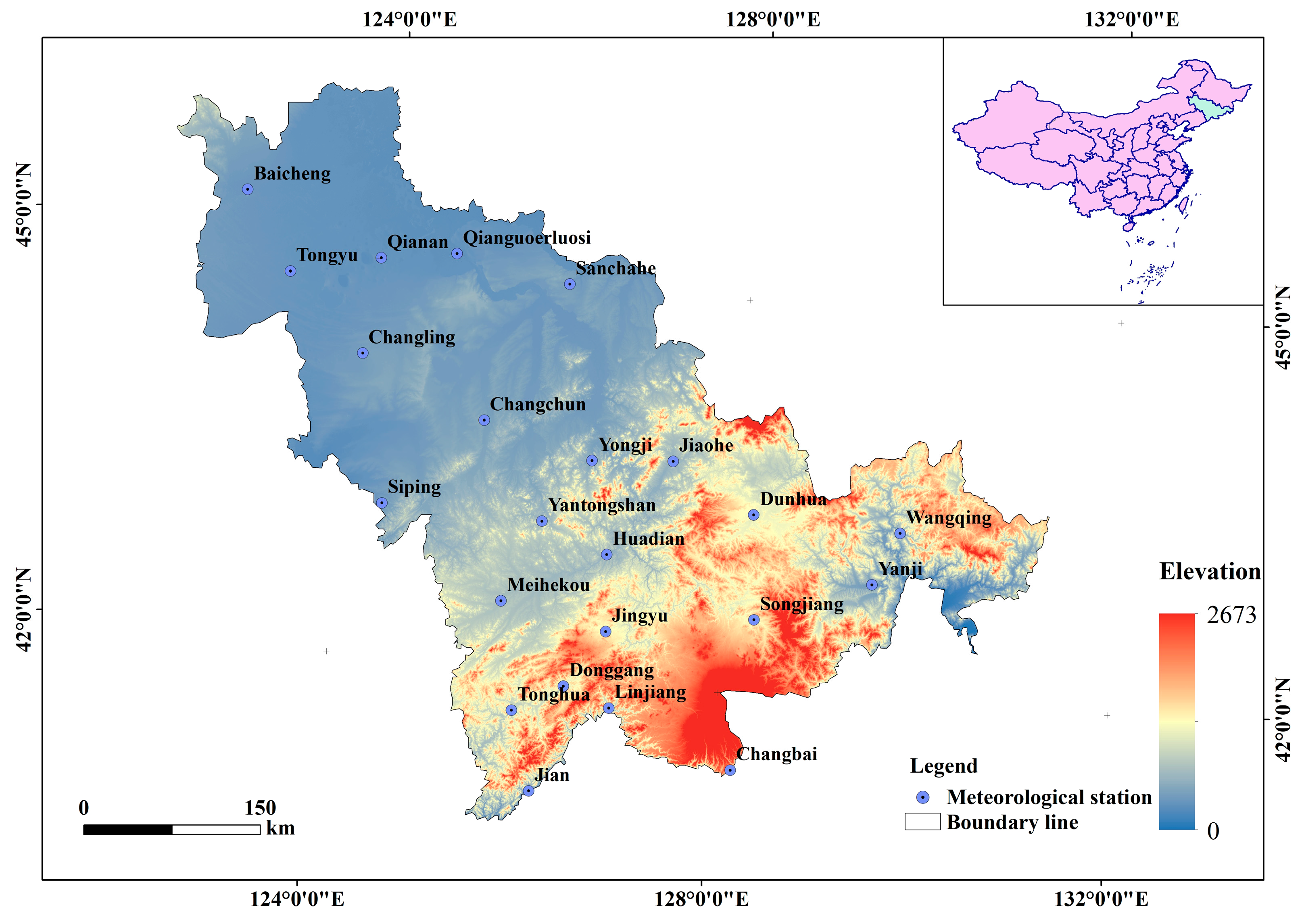
The Jilin Province is situated in the central part of Northeast China, with geographic coordinates of 40°52″–46°18″ N and 121°38″–131°19″ E. It occupies a strategic location in Northeast Asia and is surrounded by Russia, Japan, North Korea, Mongolia, South Korea, and Northeast China. Its neighboring provinces include Heilongjiang to the north and Liaoning to the south, whereas the Inner Mongolia Autonomous Region borders the province to the west. Russia lies to its east and the Tumen and Yalu rivers form its south-eastern border with the Democratic People’s Republic of Korea located across the sea. The province extends ~650 km from east to west and 300 km from north to south. The Jilin Province is characterized by two distinct landform types; the Great Black Mountains in its center divide the province into mountainous terrain to the east and plains to the west [10]. The province is located in the northern temperate zone and has an average annual precipitation ranging from 550 to 910 mm, 2200 to 3000 h of sunshine throughout the year, an annual active accumulated temperature of 2700–3600 °C, and frost-free period of 110–160 days.

The main land use types are agricultural land, forest, grassland, and construction land. The western Songliao Plain area is mainly a plain with sandy loam and sandy soils, which are loose and sandy, have poor water and fertility retention, and are prone to droughts (Figure 1).

2.2. Data

Data were obtained from the daily meteorological data series of the National Meteorological Science Data Center’s daily value dataset of China’s terrestrial climate [11]. Data include precipitation, maximum air pressure, minimum air pressure, daily average air pressure, average air temperature, minimum relative humidity, maximum air temperature, minimum air temperature, average relative humidity, maximum wind speed and wind direction, sunshine hours, maximum wind speed and direction, and average wind speed [12]. In total, 23 basic meteorological observation stations in the Jilin Province were selected and data obtained from 1960 to 2012 at the selected stations underwent strict quality control and were of good quality. To ensure the integrity of the meteorological station data series, missing data were interpolated by establishing linear relationships with data from neighboring meteorological stations.

3. Research Methodology

3.1. SPEI Calculation

SPEI is calculated as the difference between precipitation and potential evapotranspiration using a water balance equation [13]. In this study, the SPEI series was calculated on a monthly basis (SPEI-1), three-month timescale (SPEI-3), six-month timescale (SPEI-6), twelve-month timescale (SPEI-12), twenty-four-month timescale (SPEI-24), and sixty-month timescale (SPEI-60) from 1960 to 2012. The most commonly used methods are the Penman–Monteith [14] and Thornthwaite methods. Because the Penman–Monteith method is better than Thornthwaite in calculating the SPEI and is currently the most accurate method for estimating evapotranspiration [15], the Penman–Monteith method was used in this study, as recommended by the Food and Agriculture Organization of the United Nations (FAO). In this paper, the potential evapotranspiration of each site is calculated by substituting the temperature and humidity data obtained from the National Weather Science Data Center into the formula, and then the SPEI of each site is derived from the difference between the month-by-month precipitation and evapotranspiration at each site, which is calculated as follows:

(1)

Calculate the difference between monthly precipitation and potential evapotranspiration:

$$E{T}_{0i}=\frac{0.408\nabla \left(R_n-G\right)+\epsilon \frac{900}{T+273}{U}_2\left(e_c-e_d\right)}{\nabla +\epsilon \left(1+0.34U_2\right)}$$

(1)

$$D_i=P_i-E{T}_{0i},$$

(2)

where $i$ is the month, $E{T}_{0i}$ is the potential evapotranspiration (mm) $P_i$ is the monthly precipitation, $\nabla$ is the slope of the variation in temperature with the slope of the change in saturated water vapor pressure $\left(\mathrm{kPa}·{℃}^{-1}\right)$, $U_2$ is the wind speed at 2 m above the ground Wind speed at the height $\left(\mathrm{m}·{\mathrm{s}}^{-1}\right)$, $e_c$ is the saturated vapor pressure$\left(\mathrm{kPa}\right)$, $e_d$ is actual vapor pressure$\left(\mathrm{kPa}\right)$, $T$ is the average temperature $\left(℃\right)$, $\epsilon$ is the humidity Table constant $\left(\mathrm{kPa}·{℃}^{-1}\right)$, and $G$ is the soil heat flux density $\left(\mathrm{MJ}·{\mathrm{m}}^{-2}·{\mathrm{d}}^{-1}\right)$.

(2)

Aggregation and normalization of $D_i$ based on the chosen timescale:

$$\begin{gathered} D_{u,v}^k={{\displaystyle \sum }}_{m=13+v-k}^{12}{D}_{u-1,m}+{{\displaystyle \sum }}_{m=1}^v{D}_{u,m} v<k \\ {D}_{u,v}^k={{\displaystyle \sum }}_{m=v-k+1}^j{D}_{u,m}, v\ge k \end{gathered}$$

(3)

where $D_{u,v}^k$ is the cumulative precipitation evapotranspiration difference over $k$ months starting from month $v$ of year $u$.

(3)

A log-logistic distribution was used to fit a function to the $D_i$data series [16]:

$$f\left(x\right)=\frac{\mu }{\sigma }{\left(\frac{x-\gamma }{\sigma }\right)}^{\mu -1}{\left[1+{\left(\frac{x-\gamma }{\sigma }\right)}^{\mu }\right]}^{-2}$$

(4)

where $\sigma$ is the scale factor, $\mu$ is the shape factor, and $\gamma$ is the origin parameter.

$$\sigma =\frac{\left(W_0-2W_1\right)\mu }{\Gamma \left(1+\frac{1}{\mu }\right)\Gamma \left(1-\frac{1}{\mu }\right)}$$

(5)

$$\mu =\frac{\left(2W_1-W_0\right)}{6W_1-2W_0-6W_2}$$

(6)

$$\gamma =W_0-\sigma \Gamma \left(1+\frac{1}{\mu }\right)\Gamma \left(1-\frac{1}{\mu }\right),$$

(7)

where $\Gamma$ is a Gamma function on $\mu$ such that the cumulative probability for a given timescale is:

$$F\left(t\right)={\left[{\left(\frac{\sigma }{t-\gamma }\right)}^{\mu }+1\right]}^{-1}$$

(8)

Normalize the given cumulative probability distribution function. The probability of exceeding a certain timescale is $P=1-F\left(t\right)$ and the probability-weighted distance is $\omega =\sqrt{-2\ln \left(P\right)}$:

$$\left\{\begin{array}{c}SPEI=\omega -\frac{c_0+c_1\omega +c_2{\omega }^2}{1+d_1\omega +d_2{\omega }^2+d_3{\omega }^3}, p\le 0.5\\ SPEI=-\left(\omega -\frac{c_0+c_1\omega +c_2{\omega }^2}{1+d_1\omega +d_2{\omega }^2+d_3{\omega }^3}\right), p>0.5\end{array}\right.$$

(9)

where $c_0$ = 2.515517; $c_1$ = 0.802853; $c_2$ = 0.010328; $d_1$ = 1.432788; $d_2$ = 0.189269; and $d_3$ = 0.001308.

3.2. Timescale Selection

Because different timescales can represent different drought conditions, a 1-month timescale reflects short-term drought, and a 3-month timescale reflects seasonal drought conditions. SPEI values of 3, 5, 8, and 11 months were selected to represent spring, summer, autumn, and winter to study seasonal drought conditions. The SPEI values of the 12-month timescale were selected to reflect interannual drought conditions. Based on relevant studies [17] and combining with the actual drought situation in Jilin Province. The SPEI drought classifications are listed in

Table 1. SPEI drought classification.

SPEI	Grade
$\ge -0.55$	No drought
$\le -0.55$	Light drought
$\le -1.0$	Moderate drought
$\le -1.5$	Severe drought
$\le -2.0$	Extraordinary drought

.

3.3. Identification of Drought Variables

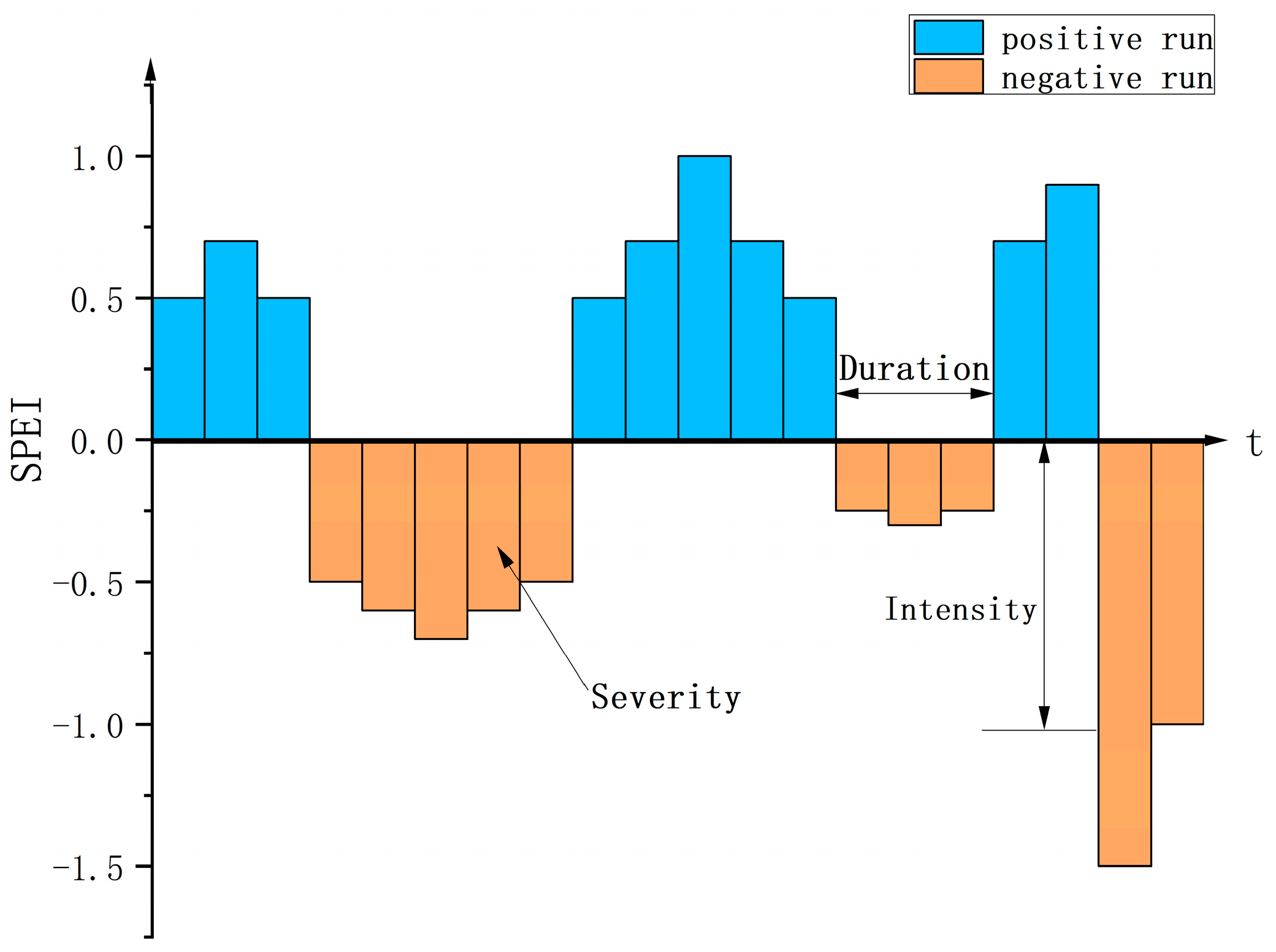
It is generally accepted that run theory (Figure 2) can be used for drought event identification, where drought duration, severity, and intensity are used as drought variables for drought risk analysis. To reduce the effect of a minor drought duration on the drought identification, the accuracy of the drought identification can be improved as follows [18]:

(1)

Drought duration (Dd): number of consecutive months in which the SPEI value is below a threshold of −0.55;

(2)

Drought severity(Ds): sum of all events within the drought duration [19];

(3)

Drought intensity (Di): absolute maximum value of the SPEI over the drought duration;

(4)

Based on the above-mentioned definitions, a drought can be judged as present when the drought index is below −0.55. If the drought event lasts for only one month and the drought index is above −0.85, the event is excluded. If the time interval between two adjacent drought events is only one month and the drought index for that month is less than zero, it is regarded as one drought event; otherwise, these two drought events are regarded as two independent drought processes [4].

3.4. Construction of Edge Distribution Functions

To construct a joint distribution function using the copula function for the three characteristics of drought duration, intensity, and severity in pairs [20], it is essential to provide definitions for the exponential, beta, extreme value, gamma, logarithmic, Weibull, and generalized extreme value distributions [21]. In addition, the Kendall and Spearman rank correlation coefficients were employed to assess the correlation between the characteristic variables, determining whether the drought variables are suitable for constructing the joint distribution function [22].

3.5. Copula Function

The copula function theory, first proposed by Sklar [23], can be used for binary or multivariate drought frequency analyses, which can be combined with a multivariate joint distribution in the interval [0,1]. Four main types of copula functions are commonly used today: Archimedean (Frank, Clayton, Gumbel), elliptic (t, Gaussian), extreme value (Husler–Reiss, t-EV), and hybrid (Plackett), each of which has its own characteristics that can be illustrated in different ways.

When any two of the variables, that is, drought duration, intensity, and severity, are selected for the analysis of the drought characteristics [24], it is necessary to measure these two variables to construct a correlation function between them. Copula functions are widely used in hydrology. The Archimedes and elliptic copula series are widely used today [25].

To make the alternative copula model more complete, 25 representative copula functions were selected to construct a joint distribution function. The parameters θ were estimated using the maximum likelihood method. The 25 kinds of copula functions including t, Gaussian 2 kinds of elliptic copula functions, Gumbel, Clayton, Frank, Tawn, Independence, Roch–Alegre, AMH, FGM, Joe, Plackett, BB1, BB5, Raftery, Cuadras–Auge, Linear–Spearman, Cubic, Shih–Louis, Burr, Galambos, Marshal–Olkin, Fischer–Kock, Nelsen, Fischer–Hinzmann, and 23 Archimedean copula functions. The range of parameter θ and joint distribution function are shown in

Table 2. Parameters of the copula function.

Copula	Equation	Parameter
Gumbel Copula	$\exp \left\{-{\left[{\left(-ln{u}_1\right)}^{\theta }+{\left(-ln{u}_2\right)}^{\theta }+{\left(-ln{u}_3\right)}^{\theta }\right]}^{\frac{1}{\theta }}\right\}$	$\theta \in \left[-1,\infty \right]$
Clayton Copula	${\left({u_1}^{-\theta }+{u_2}^{-\theta }+{u_3}^{-\theta }-3\right)}^{\frac{-1}{\theta }}$	$\theta \in \left[-1,\infty \right]$
Frank Copula	$-\frac{1}{\theta }ln\left[1+\frac{\left(e^{-\theta u_1}-1\right)\left(e^{-\theta u_2}-1\right)\left(e^{-\theta u_3}-1\right)}{{\left(e^{-\theta }-1\right)}^2}\right]$	R
Gaussian Copula	${{\displaystyle \int }}_{-\infty }^{{\varphi }^{-1\left(u\right)}}{{\displaystyle \int }}_{-\infty }^{{\varphi }^{-1\left(v\right)}}\frac{1}{2\pi \sqrt{1-{\theta }^2}}\exp (\frac{2\theta xy-x^2-y^2}{2\left(1-{\theta }^2\right)})dxd{y}^2$	$\theta \in \left[-1,1\right]$
independence	$uv$	$\theta \in \left[-1,1)\right.$
AMH	$\frac{uv}{1-\theta \left(1-u\right)\left(1-v\right)}$	$\theta \in \left[-1,\infty )\right.$
Joe	$1-{\left[{\left(1-u\right)}^{\theta }+{\left(1-v\right)}^{\theta }-{\left(1-u\right)}^{\theta }{\left(1-v\right)}^{\theta }\right]}^{\frac{1}{\theta }}$	$\theta \in \left[-1,\infty )\right.$
FGM	$uv\left[1+\theta \left(1-u\right)\left(1-v\right)\right]$	$\theta \in \left[-1,1\right]$
plackett	$\frac{1+\left(\theta -1\right)\left(u+v\right)-\sqrt{{\left[1+\left(\theta -1\right)\left(u+v\right)\right]}^2-4\theta \left(\theta -1\right)uv}}{2\left(\theta -1\right)}$	$\theta \in \left(0,\infty \right)$
Cuadras–Auge	${\left[\min \left(u,v\right)\right]}^{\theta }{\left(uv\right)}^{1-\theta }$	$\theta \in \left[0,1\right]$
Raftery	$\left\{\begin{array}{c}u-\frac{1-\theta }{1+\theta }{u}^{\frac{1}{1-\theta }\left(v^{\frac{-\theta }{1-\theta }}-v^{\frac{1}{1-\theta }}\right), if u\le v}\\ u-\frac{1-\theta }{1+\theta }{v}^{\frac{1}{1-\theta }\left(u^{\frac{-\theta }{1-\theta }}-u^{\frac{1}{1-\theta }}\right), if v\le u}\end{array}\right.$	$\theta \in \left[0,1)\right.$
Shih-Louis	$\left\{\begin{array}{c}\left(1-\theta \right)uv+\theta \min \left(u,v\right),if \theta \in \left[0,1\right]\\ \left(1-\theta \right)uv+\theta n\left(u+v-1\right)\psi \left(u+v-1\right),if \theta ϵ\left(-\infty ,\left.0\right]\right.\end{array}\right.$ $\psi \left(a\right)=1 if a\ge 0 if\psi \left(a\right)=0 if a<0$	$\theta \in \left[0,1\right]$
Cubic	$uv\left[1+\theta \left(u-1\right)\left(v-1\right)\left(2u-1\right)\left(2v-1\right)\right]$	$\theta \in \left[-1,2\right]$
Burr	$uv\exp {\left\{{\left(-\ln \left(u\right)\right)}^{-\theta }+{\left(-\ln \left(v\right)\right)}^{-\theta }\right\}}^{\frac{-1}{\theta }}$	$\theta \in \left(0,\infty \right)$
Nelsen	$\frac{-1}{\theta }log\left\{1+\frac{\left[\exp \left(-\theta u\right)-1\right]\left[\exp \left(-\theta v\right)-1\right]}{\exp \left(-\theta \right)-1}\right\}$	$\theta \in \left(0,\infty \right)$
Galambos	$uv\exp {\left\{{\left(-\ln \left(u\right)\right)}^{-\theta }+{\left(-\ln \left(v\right)\right)}^{-\theta }\right\}}^{\frac{-1}{\theta }}$	$\theta \in \left[0,\infty )\right.$
Marshall–Olkin	$\min \left[u^{\left(1-{\theta }_1\right)}v,u{v}^{\left(1-{\theta }_2\right))}\right]$	${\theta }_1,{\theta }_2\in \left[0,\infty )\right.$
Fischer–Hinzmann	$uv\left[1+{\theta }_2\left(1-u^{\frac{1}{{\theta }_1}}\right)\left(1-v^{\frac{1}{{\theta }_1}}\right)\right]$	${\theta }_1\in \left(0,\infty \right),{\theta }_2\in R$
Roch–Alegre	$\exp \left\{{\left[{({(1-\ln \left(u\right))}^{{\theta }_1}-1)}^{{\theta }_2}+{\left({(1-\ln \left(v\right))}^{{\theta }_1}-1\right)}^{{\theta }_2}{}^{\frac{1}{{\theta }_2}}+1\right]}^{\frac{1}{{\theta }_1}}\right\}$	${\theta }_1\in \left(0,\infty \right)$, ${\theta }_2\in \left[1,\infty )\right.$
Fischer–Kock	$uv{\left[1+{\theta }_2(1-u^{\frac{1}{{\theta }_1}})(1-v^{\frac{1}{{\theta }_1}})\right]}^{{\theta }_1}$	${\theta }_1\in \left[1,\infty )\right.,{\theta }_2\in \left(0,\infty \right)$
BB1	${\left\{1+{\left(u^{-{\theta }_1}-1\right)}^{{\theta }_2}+{\left(u^{-{\theta }_1}-1\right)}^{\frac{1}{{\theta }_2}}\right\}}^{\frac{-1}{{\theta }_1}}$	${\theta }_1\in \left(0,\infty \right),{\theta }_2\in \left(1,\infty \right)$
BB5	$\exp \left\{-{\left[(-\ln {\left(u\right)}^{{\theta }_1}+(-\ln {\left(v)\right)}^{{\theta }_1}-{(-\ln {\left(u\right)}^{-{\theta }_1{\theta }_2})}^{\frac{-1}{{\theta }_2}}\right]}^{\frac{1}{{\theta }_1}}\right\}$	${\theta }_1\in \left[1,\infty )\right.,{\theta }_2\in \left(0,\infty \right)$
Tawn	$\exp \left\{\ln \left(u^{1-{\theta }_1}\right)+\ln \left(v^{1-{\theta }_2}\right)-{[{\left(-{\theta }_1\ln \left(u\right)\right)}^{{\theta }_3}+{\left(-{\theta }_2\ln \left(v\right)\right)}^{{\theta }_3}]}^{\frac{1}{{\theta }_3}}\right\}$	${\theta }_1,{\theta }_2\in \left[0,1\right],{\theta }_3\in \left[1,\infty )\right.$
t	${{\displaystyle \int }}_{-\infty }^{t_{{\theta }_2}^{-1}\left(u\right)}{{\displaystyle \int }}_{-\infty }^{t_{{\theta }_2}^{-1}\left(v\right)}\frac{\mathsf{\Gamma }\left(\frac{{\theta }_2+2}{2}\right)}{\mathsf{\Gamma }\left({\theta }_2+2\right)\pi {\theta }_2\sqrt{1-{\theta }_1^2}}{\left(1+\frac{x^2-2xy{\theta }_1+y^2}{{\theta }_2}\right)}^{\frac{({\theta }_2+2)}{2}}dxd{y}^c$	${\theta }_1\in \left[-1,1\right]and{\theta }_2\in \left[0,\infty \right]$
Linear-Spearman	$\left\{\begin{array}{c}\begin{array}{c}\left[u+\theta \left(1-u\right)\right]v, if v\le u and \theta \in \left[0,1\right]\\ \left[v+\theta \left(1-v\right)\right]u, if u<v and \theta \in \left[0,1\right]\end{array}\\ \begin{array}{c}\left(1+\theta \right)uv, if u+v<1 and \theta \in \left[-1,0\right]\\ uv+\theta \left(1-u\right)\left(1-v\right), if u+v\ge 1 and \theta \in \left[-1,0\right]\end{array}\end{array}\right.$	$\theta \in \left[-1,1\right]$

[26].

3.5.1. Estimation of parameters

The copula parameters are calculated using parametric and nonparametric estimation methods such as the maximum likelihood function method, correlation index method, and marginal inference function estimation method. The latter is the nonparametric method used in this paper. It is mainly related to the copula parameters θ correlation, θ and τ (Kendall correlation coefficient), as shown in the following equation in

Table 3. Parameters of the copula function.

Copula Function	Relation between θ and τ	Scope of Use
Gumbel Copula	$\tau =1-\frac{1}{\theta }$	Positive correlation
Clayton Copula	$\tau =\frac{\theta }{\left(\theta +2\right)}$	Positive correlation
Frank Copula	$\tau =1+\frac{4}{\theta }({{\displaystyle \int }}_0^{\theta }\frac{t}{e^t-1}dt-1)$	Positive/negative correlation

. After calculating τ from the data, we can derive the parameters of the joint distribution.

3.5.2. Validation and Evaluation

The degree of fit is an important criterion for choosing the joint probability distribution of the copula function. Common evaluation methods include the Akaike information criterion (AIC) and the Bayesian information criterion (BIC), Nash–Sutcliffe efficiency (NSE), root-mean-square error, and graphical evaluation analysis [27]. In this study, the root-mean-square error method, NSE coefficient method, and AIC were chosen as the best-fit tests to assess the fit and select the appropriate copula function [28].

$$MSE=\frac{1}{a-b}{\displaystyle \sum }_{i=1}^b{\left[p_c\left(i\right)-p_0\left(i\right)\right]}^2$$

(10)

$$RMSE=\sqrt{\frac{1}{b}{\displaystyle \sum }_{i=1}^b{\left[p_c\left(i\right)-p_0\left(i\right)\right]}^2}$$

(11)

$$AIC=blnMSE+2a$$

(12)

$$NSE=1-\frac{{{\displaystyle \sum }}_{i=1}^b{\left[p_c\left(i\right)-p_0\left(i\right)\right]}^2}{{{\displaystyle \sum }}_{i=1}^b{\left[p_c\left(i\right)-\overline{p_c\left(i\right)}\right]}^2},$$

(13)

where $b$ is the number of drought epochs or intensities in the calculated data, $MSE$ is the mean squared error, $AIC$ is the criterion for the amount of information in the red pool, $RMSE$ is the root-mean-square error, $p_0\left(i\right)$ is the empirical value of the multivariate joint probability distribution of the copula function, $p_c\left(i\right)$ is the calculated value of the multivariate joint probability distribution of the copula function, and $a$ is the number of model parameters. The smaller the value of the objective function $AIC$ is, the closer is the $RMSE$ to zero. The closer the $NSE$ value is to one, the better is the copula function simulation effect.

3.5.3. Drought Event Recurrence Period

The use of return periods to describe the time period of catastrophic events has been limited to a single factor; however, the analysis of the return period of a single factor often leads to errors in the evaluation of catastrophic events, making them potentially dangerous. Many natural phenomena are the result of a combination of factors and the occurrence of droughts is also the result of a combination of factors. A binary return period was used to characterize the drought severity [29].

$$T_{c2}=\frac{M}{mP\left(D\ge d\cap S\ge s\right)}=\frac{M}{m\left[1-e-f+C\left(e,f\right)\right]},$$

(14)

where $T_{c2}$ is the joint recurrence period of the bivariate ($D\ge d$ or $S\ge s$); $m$ is the number of drought occurrences in the time period; $M$ is the series length; and $C\left(e,f\right)$ represents the joint probability of the two-dimensional set of variables [30].

If the severity of the drought is portrayed according to the trivariate recurrence period:

$$T_{c3}=\frac{M}{mP\left(D\ge d\cup S\ge s\cup I\ge i\right)}=\frac{M}{m\left[1-C\left(e,f,g\right)\right]},$$

(15)

where $T_{c3}$ is the joint recurrence period of the three variables, and $C\left(e,f,g\right)$ represents the joint probability of the three-dimensional set of variables.

4. Results

4.1. Mann–Kendall Trend Test for Drought Events in the Study Area

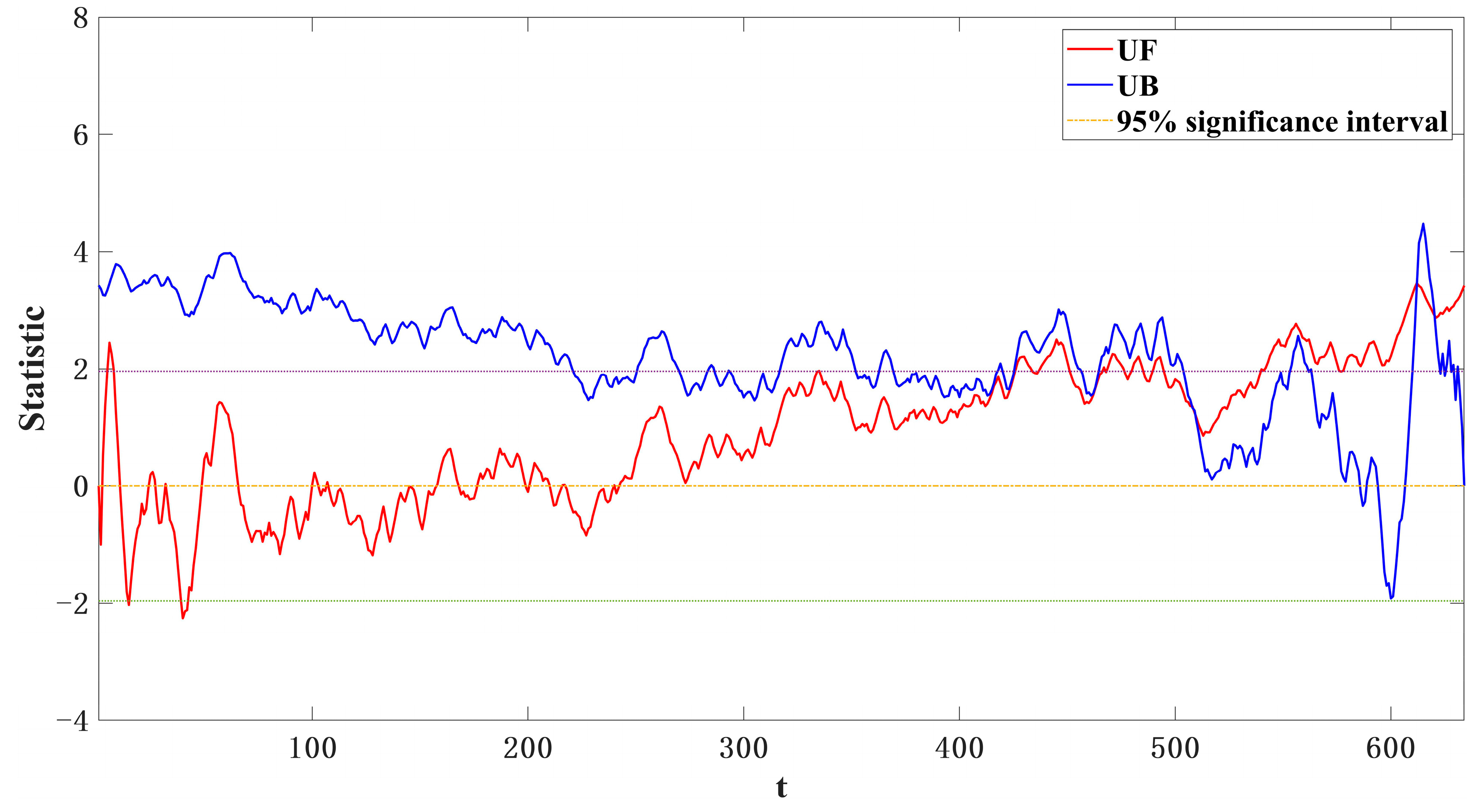
Through the comprehensive analysis of the data from several meteorological stations in Jilin Province (Figure 3), we derived the overall trend and sudden change in the SPEI-3 index in Jilin Province, and carefully verified and compared the data from other meteorological stations in Jilin Province, whose trend test results basically remained the same with that of the Meihekou station, and in addition, the Meihekou station has a more representative climatic and geographic condition due to its location in the core area of Jilin Province, as well as a more complete historical observation record [31]. The mutation results are shown below. A Standard Normal Distribution Statistics (UF) above zero represents an upward trend in the series; a UF below zero represents a downward trend in the series [32]; and a UF exceeding the yellow dotted line shown represents an upward or downward trend at a level of 0.05. The intersection of the UK and UB curves indicates the location of the mutation point. The intersection of the UK and UB curves represents the point of abrupt change [31]. The graph shows that the SPEI for the Meihekou area was unstable around 2000 and 2010, with abrupt changes.

4.2. SPEI Trends at Different Timescales

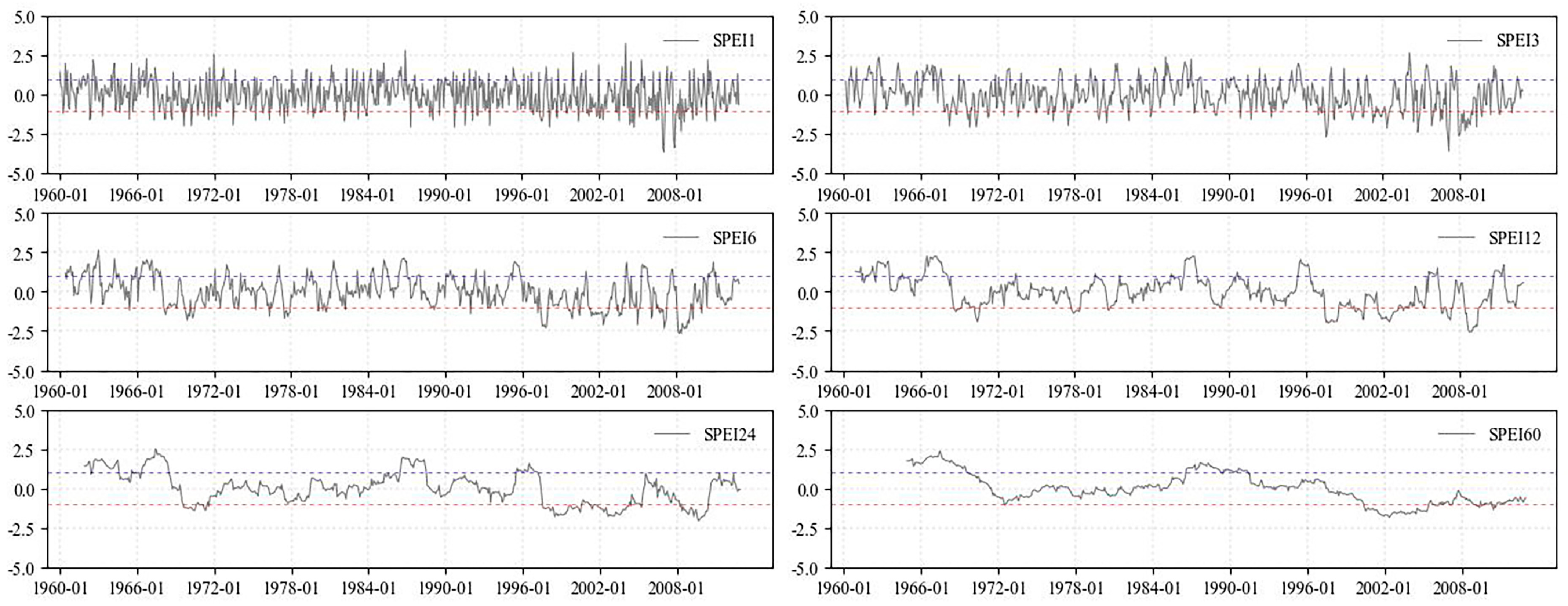
The SPEI at different timescales better reflects drought characteristics. Due to the large number of study sites, the timescale of the Changbai region was chosen for the analysis (Figure 4). The graph shows some similarities in the changes at different time scales: the SPEI values at each timescale are mostly negative. At the timescale of one month, a high frequency of fluctuations was observed, with a very short period. It can be speculated that these phenomena were caused by various drought influences and that the period of the drought fluctuation becomes longer at different timescales, such as three, six, and twelve months, and the frequency and severity of occurrence decreases. However, the drought duration extends, with several droughts occurring between 1968 and 1970 on the one-month timescale and to some extent at ~1990. The 2006–2008 was the most severe drought period [33]. At other timescales, droughts occurred over the same period, all around 2008. From the above, it can be concluded that climate change was stable between 1972 and 1984, with significant changes occurring between 1968 and 1972 and between 1996 and 2002. Overall, the timing of the drought occurrence is similar across the different timescales; as the timescale increases, the drought range and duration increase [34], the frequency of drought events declines while the drought duration increases.

Because short timescales are not sufficient for the determination of drought-influencing factors and timescales that are too long cannot explain changes within a certain period, in this study, a three-month SPEI timescale was used for the analysis of drought conditions.

4.3. Drought Frequency Map

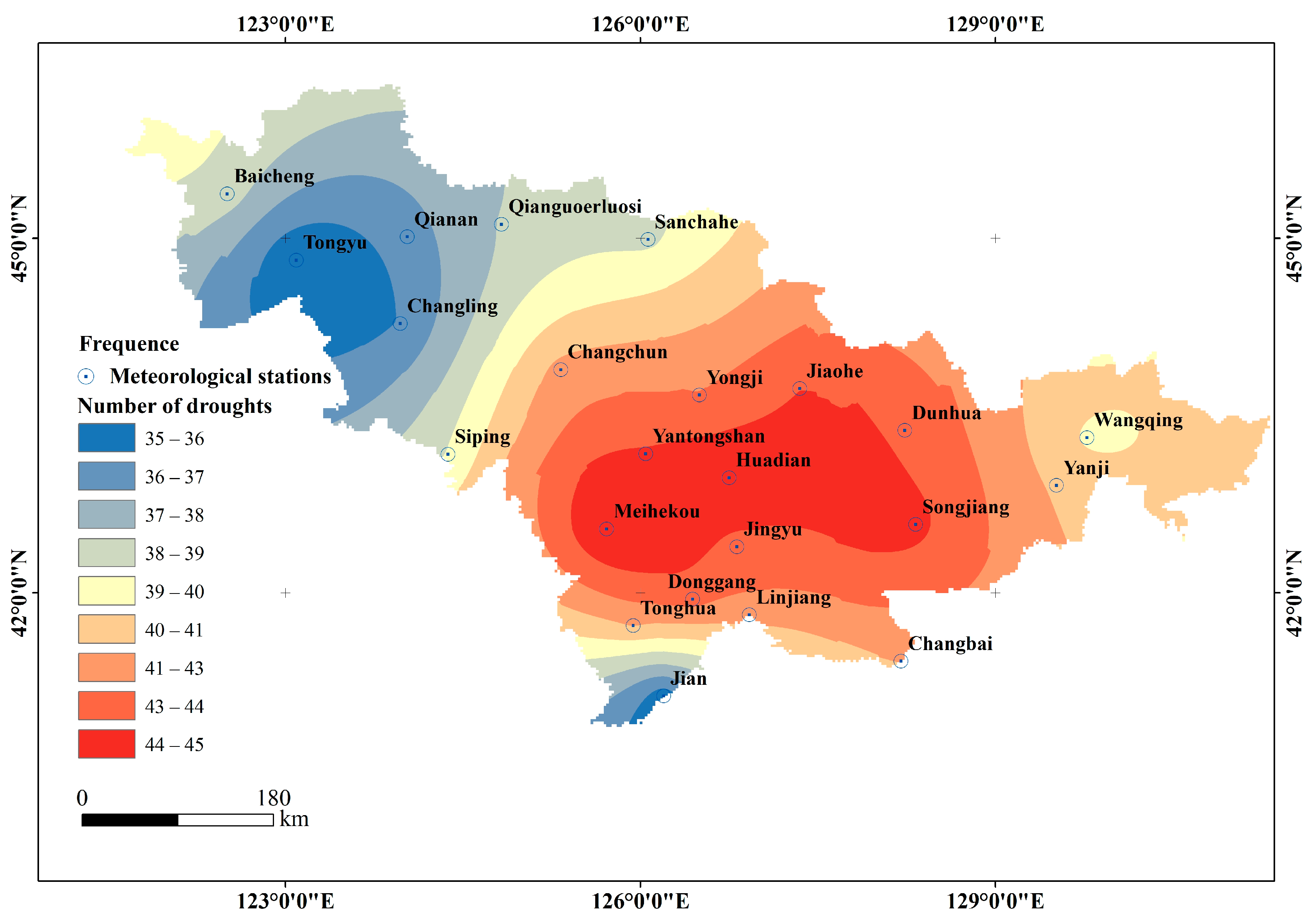
The number of droughts occurring in each region was obtained from theoretical results for the Jilin Province. The kriging interpolation method in ArcGIS was used to spatially interpolate drought events occurring at each station (Figure 5). The color blue indicates that the number of droughts is low, and the color red indicates that the number of droughts is high. The graph shows that the number of droughts occurring in the northwestern and southwestern Jilin Province is low, averaging 36 times, whereas the number of droughts occurring in the southcentral Jilin Province is high [35], averaging 43 times. Therefore, such factors must be considered when formulating relevant drought prevention and relief strategies and measures should be implemented in drought-prone areas.

4.4. Correlation Analysis of Drought Characteristic Variables

After identifying the drought characteristic variables using run theory, the Kendall, Spearman, and Pearson product–moment correlation coefficients between the two variables were analyzed to determine the correlations between the variables. When the coefficient of the two variables approaches 1, the correlation strengthens. The results of the study are shown in

Table 4. Correlation coefficients for drought variables.

Sites	Variables	Kendall	Spearman	Pearson
Baicheng	Ds-Dd	−0.7717	−0.8983	−0.9209
	Ds-Di	−0.5075	−0.5787	−0.4884
	Dd-Di	0.4927	0.6436	0.6719
Donggang	Ds-Dd	−0.7400	−0.8621	−0.8671
	Ds-Di	−0.5893	−0.5169	−0.6838
	Dd-Di	0.5981	0.7828	0.5430
Dunhua	Ds-Dd	−0.7771	−0.8962	−0.9507
	Ds-Di	−0.5589	−0.4078	−0.5789
	Dd-Di	0.5693	0.5965	0.6306
Huadian	Ds-Dd	−0.7897	−0.9194	−0.8585
	Ds-Di	−0.6609	−0.5145	−0.6684
	Dd-Di	0.6394	0.5498	0.5302
Jian	Ds-Dd	−0.9149	−0.9806	−0.9899
	Ds-Di	−0.6254	−0.6792	−0.5812
	Dd-Di	0.6256	0.7966	0.6594

Notes: Dd represents the duration of the drought event, Ds represents the severity of the drought, Di is the intensity of the drought.

. Because of the large number of study sites, only some results are listed in the table.

4.5. Determination of Marginal Functions

Before constructing the copula function, an appropriate marginal distribution function was selected for each variable and a fitting method was used to fit the drought variables to obtain the optimal marginal distribution function and its parameter values. The marginal distribution function and variables are listed in

Table 5. Marginal distribution functions and parameter values corresponding to drought variables.

Sites	Variables	Functions	Parameters	Parameter Values
Baicheng	Ds	Generalized Pareto	k	25.6490
			sigma	0
			theta	2.0000
	Dd	Generalized Pareto	k	−1.6897
			sigma	29.9207
			theta	−18.8192
	Di	Extreme value	mu	−0.9606
			sigma	0.2529
Donggang	Ds	Generalized Pareto	k	25.3034
			sigma	0
			theta	2.0000
	Dd	Generalized Pareto	k	−1.4288
			sigma	15.7230
			theta	−12.2377
	Di	Extreme value	mu	−0.9585
			sigma	0.2708
Dunhua	Ds	Generalized Pareto	k	21.1151
			sigma	0
			theta	2.0000
	Dd	Generalized extreme value	k	−1.0240
			sigma	3.3502
			mu	−4.4327
	Di	Normal	mu	−1.1935
			sigma	0.3151
Huadian	Ds	Generalized extreme value	k	4.9863
			sigma	0.4323
			mu	2.0867
	Dd	Generalized pareto	k	−1.3016
			sigma	14.9391
			mu	−12.6568
	Di	Extreme value	mu	−0.9728
			sigma	0.2406
Jian	Ds	Generalized pareto	k	−0.0179
			sigma	5.1249
			theta	2.0000
	Dd	Generalized pareto	k	−1.5899
			sigma	43.2421
			theta	−28.3157
	Di	Generalized pareto	k	−0.7778
			sigma	0.6494
			theta	−1.3801

Notes: Dd represents the duration of the drought event, Ds represents the severity of the drought, Di is the intensity of the drought.

[36].

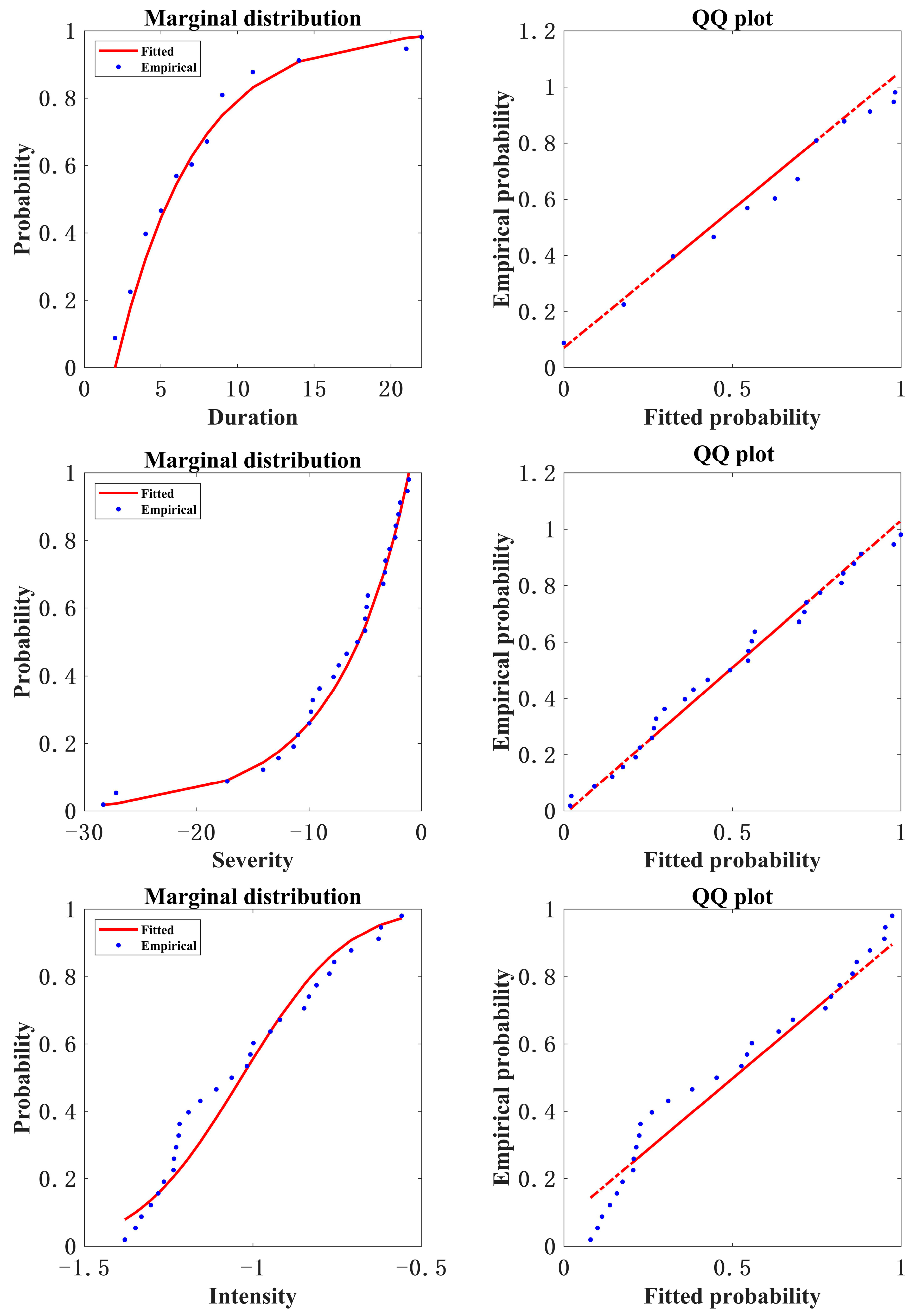
The graph below shows the fitted curve of the marginal distribution function and the quantile (Q–Q) curve for the three drought indicators in the Ji’an area (Figure 6). Based on the graph, the curve is well-fitted [37].

4.6. Selection of the Optimal Copula

The fitting effect of the copula function was tested by calculating the RMSE and NSE values of the three drought variables [38]. The closer the NSE value of the objective function is to 1 and the closer the RMSE value is to 0, the better the copula function can be simulated [39]. The results are listed in

Table 6. Selection of two-dimensional copula functions.

	Variables	Copula Function	RMSE	NSE
Jian	Ds-Dd	Gaussian	0.1975	0.4897
		t	0.1977	0.4885
		Clayton	0.6425	−4.3995
		Frank	0.1916	0.5199
		Gumbel	0.6426	−4.4008
		Independence	0.6424	−4.3988
		AMH	0.4836	−2.0586
		Joe	0.6424	−4.3988
		FGM	0.4473	−1.6171
		Plackett	0.1942	0.5065
		Cuadras–Auge	0.6425	−4.3990
		Raftery	0.6424	−4.3988
		Shih-Louis	0.3042	−0.2102
		Linear-Spearman	0.2041	0.4549
		Cubic	0.6033	−3.7611
		Burr	0.4948	−2.2023
		Nelsen	0.1916	0.5199
		Galambos	0.6424	−4.3988
		Marshal–Olkin	0.6424	−4.3988
		Fischer–Hinzmann	0.6424	−4.3988
		Roch–Alegre	0.3311	−0.4337
		Fischer–Kock	0.4501	−1.6500
		BB1	0.4528	−1.6824
		BB5	0.6430	−4.4085
		Tawn	0.6424	−4.3988
Jian	Ds-Di	Gaussian	0.2257	0.8616
		t	0.2262	0.8609
		Clayton	0.2888	0.7734
		Frank	0.2244	0.8631
		Gumbel	0.2888	0.7733
		Independence	0.2888	0.7734
		AMH	0.2260	0.8612
		Joe	0.2887	0.7734
		FGM	0.2222	0.8659
		Plackett	0.2258	0.8615
		Cuadras–Auge	0.2887	0.7734
		Raftery	0.2887	0.7734
		Shih-Louis	0.2379	0.8462
		Linear-Spearman	0.2398	0.8436
		Cubic	0.2887	0.7734
		Burr	0.2957	0.7623
		Nelsen	0.2244	0.8631
		Galambos	0.2887	0.7734
		Marshal–Olkin	0.2887	0.7734
		Fischer–Hinzmann	0.2887	0.7734
		Roch–Alegre	0.2257	0.8615
		Fischer–Kock	0.2222	0.8659
		BB1	0.2895	0.7723
		BB5	0.2887	0.7734
		Tawn	0.2887	0.7734
Jian	Dd-Di	Gaussian	0.2935	0.9673
		t	0.2943	0.9672
		Clayton	0.3056	0.9646
		Frank	0.2974	0.9665
		Gumbel	0.2965	0.9667
		Independence	0.3961	0.9405
		AMH	0.3038	0.9650
		Joe	0.3018	0.9655
		FGM	0.3009	0.9657
		Plackett	0.3002	0.9658
		Cuadras–Auge	0.3195	0.9613
		Raftery	0.3137	0.9627
		Shih-Louis	0.3219	0.9607
		Linear-Spearman	0.3219	0.9607
		Cubic	0.3942	0.9411
		Burr	0.2980	0.9663
		Nelsen	0.2974	0.9665
		Galambos	0.2948	0.9670
		Marshal–Olkin	0.2357	0.9789
		Fischer–Hinzmann	0.3185	0.9615
		Roch–Alegre	0.2956	0.9669
		Fischer–Kock	0.3031	0.9656
		BB1	0.2957	0.9668
		BB5	0.2948	0.9670
		Tawn	0.2516	0.9670

Notes: Dd represents the duration of the drought event, Ds represents the severity of the drought, Di is the intensity of the drought.

(only a portion of the results is displayed in the restricted space).

4.7. Drought Risk Assessment

4.7.1. Two-Dimensional Copula Distribution

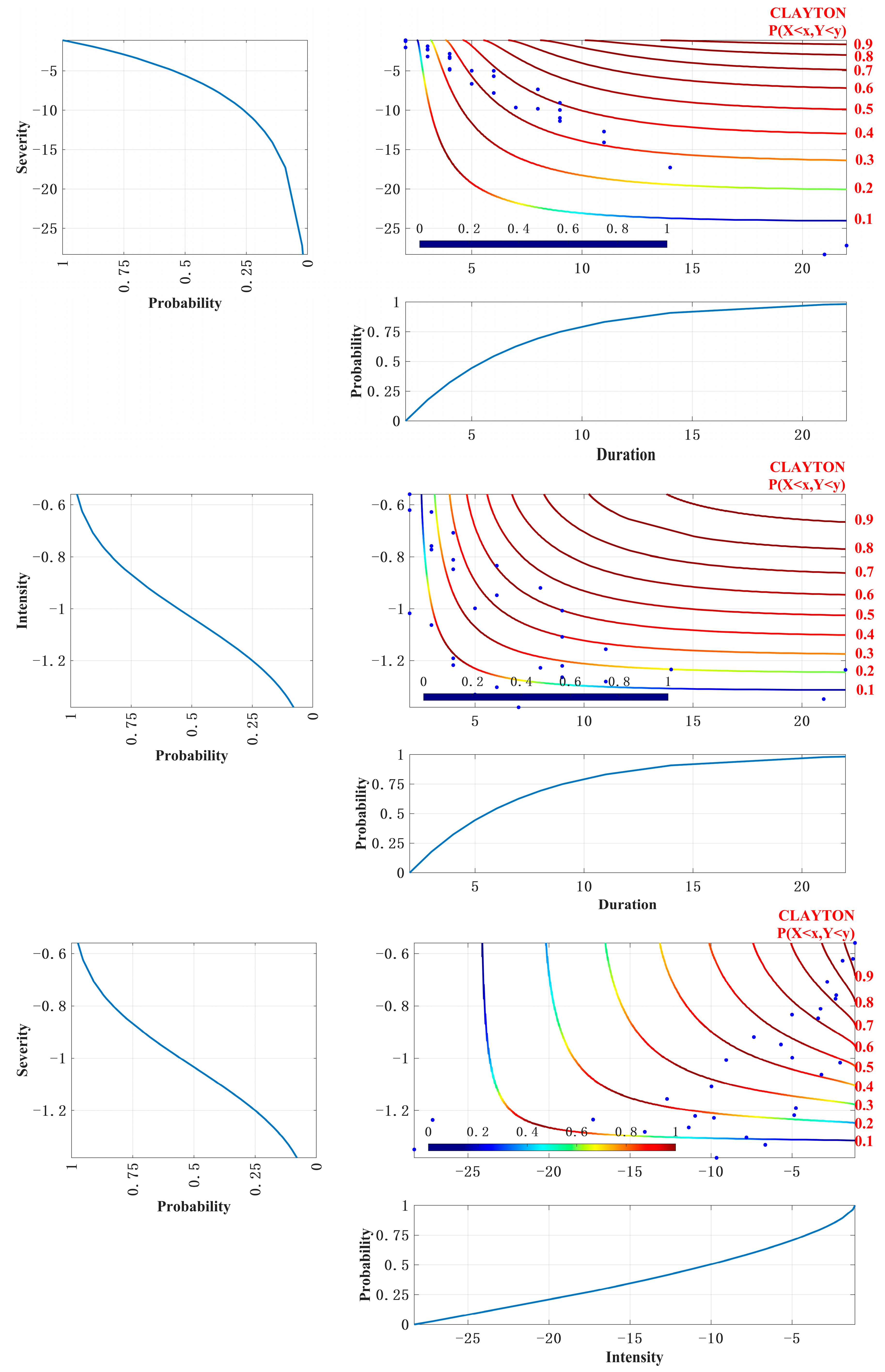
To understand the distribution characteristics of the two-dimensional joint probability, Jian drought characteristic variables (duration–severity, duration–intensity, and severity–intensity) were used as examples in this study (Figure 7). Figure 7 shows that the three groups of variables have their own distribution characteristics, where the duration–severity is uniformly distributed between 0.3 and 0.9, duration–intensity is mainly concentrated between 0.1 and 0.5, and severity–intensity is above 0.1. The joint cumulative probability of drought increases as the value of the drought variable increases. Contours are less dense when the value of the drought variable is small than when the drought variable is large. A few long-duration droughts have a high drought severity. Long-duration droughts with a high drought intensity were not observed. It is easier to have shorter-duration droughts with high or low intensity as well as shorter-duration droughts with high severity. The joint probability of the occurrence of higher intensity and severity is high.

4.7.2. Three-Dimensional Copula Distribution

In most current drought studies, a two-dimensional joint distribution is established between drought duration and drought intensity or severity; however, a three-dimensional copula model better reflects drought characteristics. A three-dimensional copula of Gumbel, Frank, and Joe and Clayton was used to construct a joint distribution of drought variables for each region of the Jilin Province to ensure the comprehensiveness of the study results.

Table 7. Choice of 3D copula functions.

Variables	Region	Copula Function	Parameter Values	AIC
Ds-Dd-Di	Baicheng	Frank	3.4317	344.7343
		Gumbel	1.8256	−61.3494
		Clayton	0.4865	191.4069
		Joe	1.1032	119.7317
	Donggang	Frank	2.8241	463.8857
		Gumbel	1.2660	−71.1607
		Clayton	0.4328	295.4420
		Joe	0.9858	219.6670
	Dunhua	Frank	2.6529	632.0213
		Gumbel	2.1977	−10.6531
		Clayton	0.4666	462.9585
		Joe	2.0011	417.7176
	Huadian	Frank	2.6432	549.5227
		Gumbel	2.2216	−21.7342
		Clayton	0.5112	369.1368
		Joe	0.8468	305.8285
	Jian	Frank	1.3527	280.2043
		Gumbel	0.6340	8.7043
		Clayton	0.8147	165.6284
		Joe	0.6424	125.7899

Notes: Dd represents the duration of the drought event, Ds represents the severity of the drought, Di is the intensity of the drought.

shows that the AIC test value of the Gumbel copula function is the smallest of the four copula functions [40]; therefore, this function fits the joint distribution of the drought characteristic variables for each region of the Jilin Province very well.

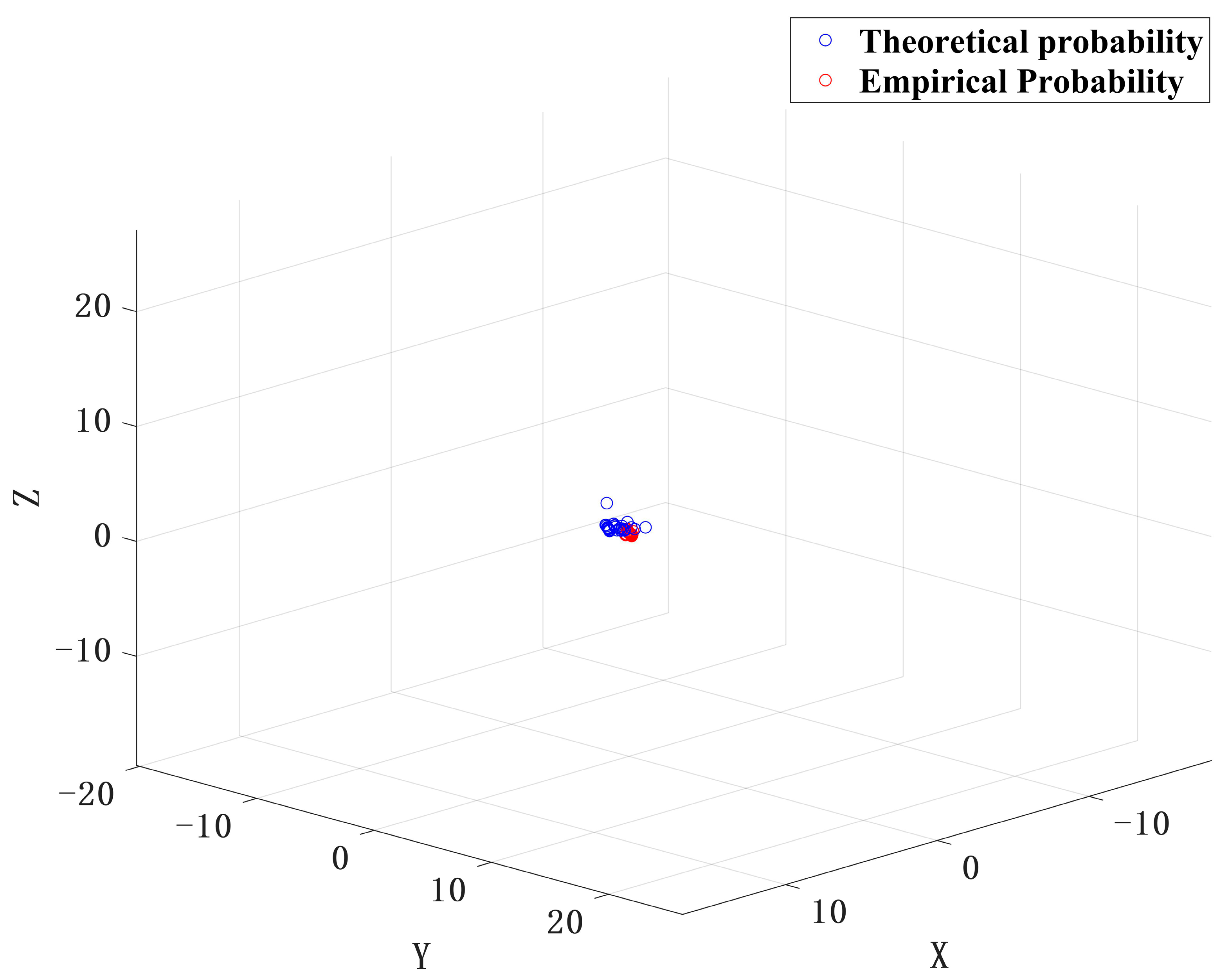
The Gumbel copula function was chosen to create a three-dimensional joint distribution, which was plotted as a comparison of the theoretical and empirical probabilities of the three-dimensional joint distribution, as seen in the following plots, which fit the model relatively well [41] (Figure 8).

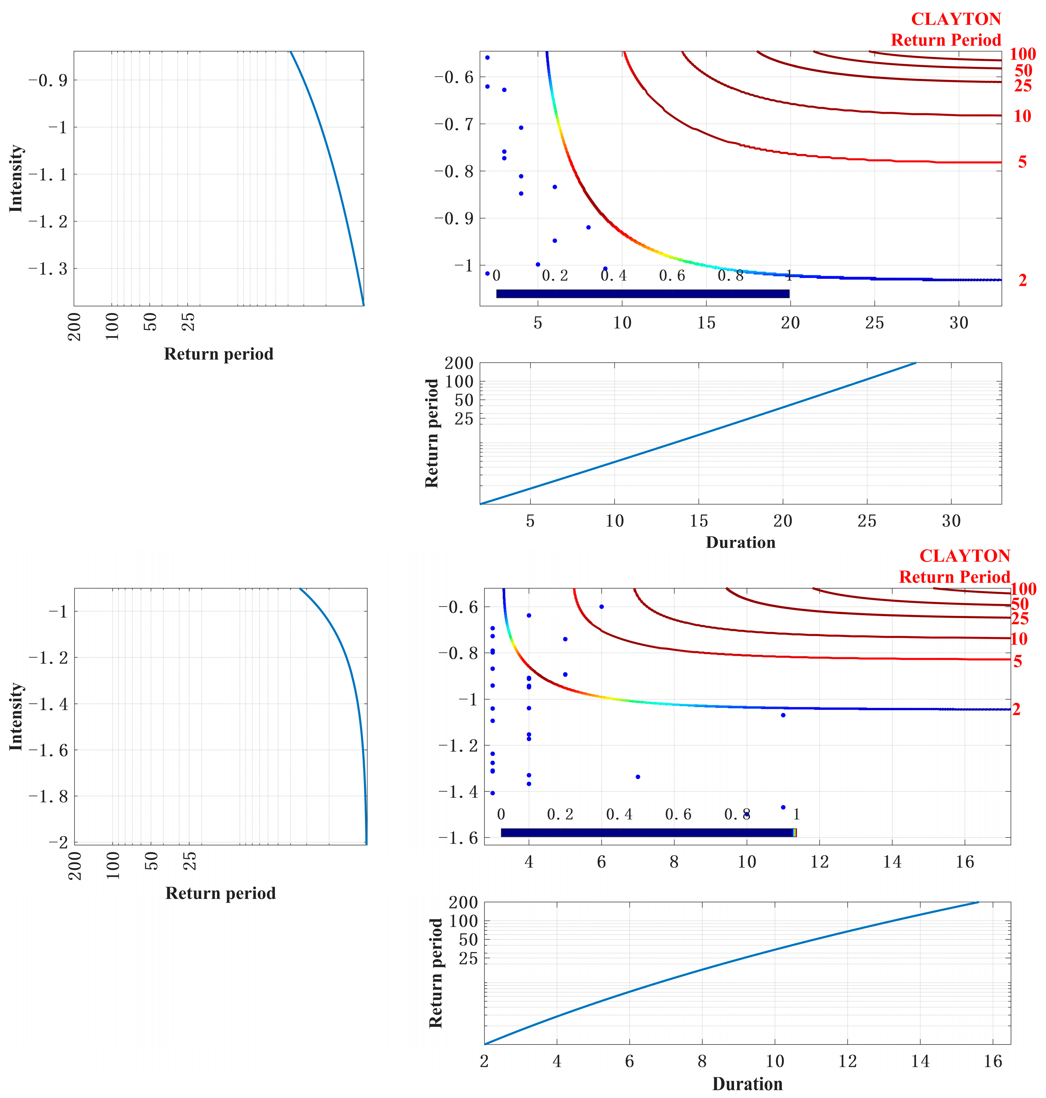
4.8. Drought Event Recurrence Period

A more detailed analysis of drought can be performed by calculating the recurrence period of drought. Firstly, the two-dimensional joint return period is calculated [42]. Figure 9 shows the time and intensity of droughts in Jian City and Jingyu County. The figure shows that the regional joint return period increases with increasing drought duration and intensity, but most of the return periods are relatively short [43]. For example, the return period in Jian City is generally less than or equal to two years, whereas the return period in Jingyu County is mostly within two years, with a maximum of ten years, indicating a lower probability of long, high-intensity droughts in both areas within the same recurrence period.

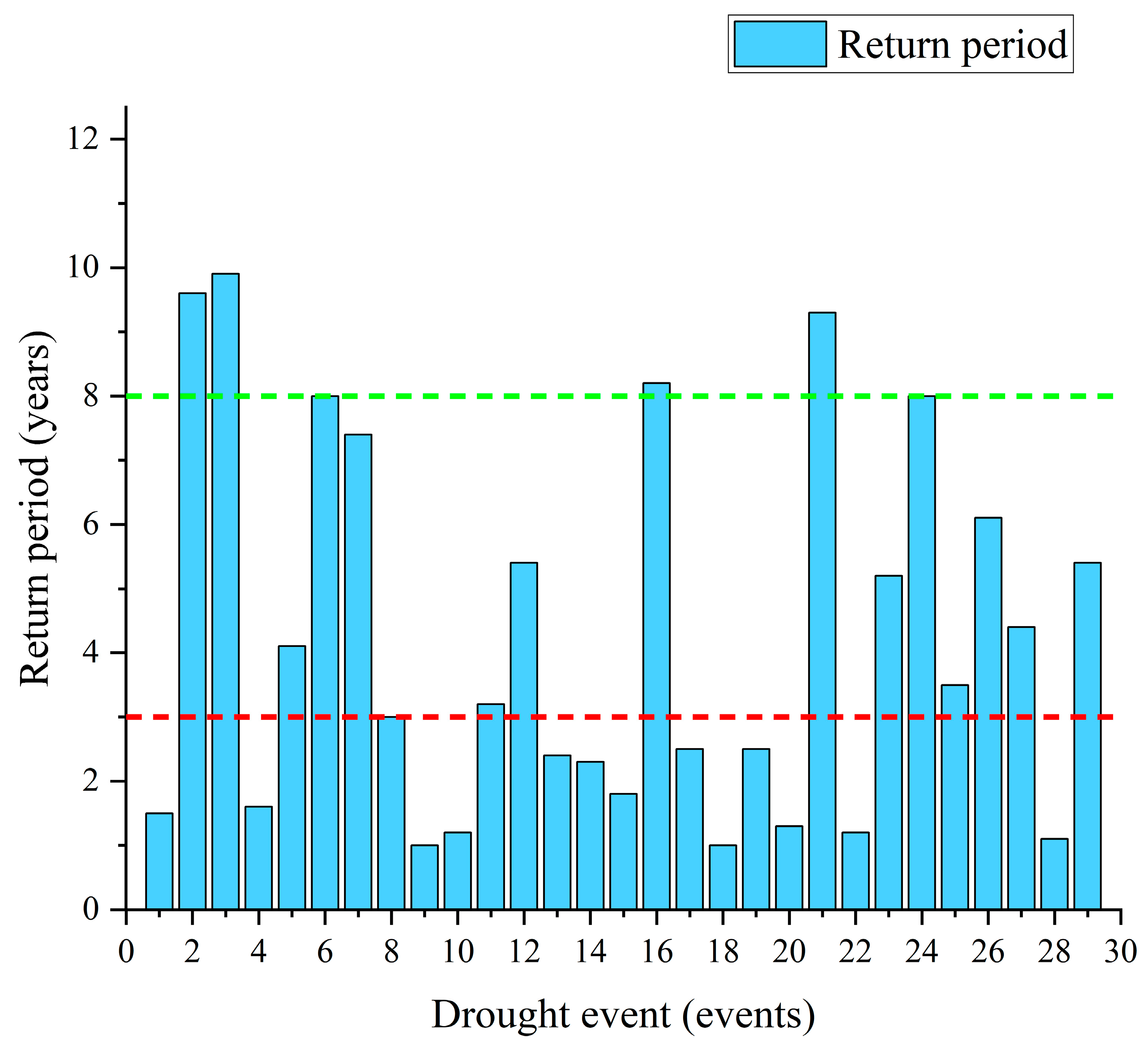
The three-dimensional joint return period was calculated for each type of drought event [44]. The results are shown in Figure 10. The figure shows that the return periods for all types of drought events defined by the drought intensity, duration, and severity are mostly below three years, with fewer periods between three and eight years and nearly no return period above ten years.

5. Discussion

Our study is consistent with the two-dimensional joint distribution analysis of drought variables in China, but we compared 25 copula functions in selecting the optimal drought variables, which enhanced the reliability of our study. In addition, we introduced a three-dimensional copula function to comprehensively assess drought risk, combining drought intensity, duration, and severity. This approach fits with the idea of using a hybrid machine learning–copula approach to estimate the probability of drought propagation in recent studies [45], which further enriches our understanding of drought dynamics [46].

In this study, SPEI values for one, three, six, twelve, twenty-four, and sixty months were calculated based on relevant data from various meteorological stations in the Jilin Province. SPEI-3 was selected to identify travel theory drought variables. In different studies, different cutoff levels were set when using run theory for drought variable identification. In this study, a single threshold was used as the cutoff level, which may cause an increase in the inaccuracy of drought event identification. Therefore, multiple threshold levels should be set in the future to enhance the precision of extracting drought features and identifying drought events. Different timescales define different drought events; SPEI-1, SPEI-3, and SPEI-12 indicate short-term, seasonal, and annual drought, respectively. Therefore, one can choose to use other SPEI timescales for copula analysis and the drought risk can be analyzed based on a combination of different SPEI timescales and new drought variables [47]. In contrast to the Bayesian Copula Multivariate Analysis (BMAViC) method [48], although our study did not directly adopt the Bayesian approach, we considered the suggestion that multiple threshold levels should be set in the future to improve the accuracy of extracting drought characteristics and identifying drought events. This is in line with the idea of the BMAViC method in improving the accuracy of drought risk assessment.

Drought is a three-dimensional phenomenon that develops simultaneously in time and space. Therefore, it is crucial to identify the core of drought occurrence and the geographic areas it affects, as well as to analyze the spatial and temporal evolutionary patterns of drought. Future research can provide insights into drought propagation patterns and evolution by mapping the spatial and temporal distribution of droughts through the use of more meteorological station data and remote sensing techniques. This will help to improve the early warning and management of drought disasters and thus better protect the agricultural and ecological environments.

In addition, our study focuses on the use of SPEI indices to identify drought variables, especially SPEI-3 as an indicator of drought variables. However, we also note the use of the Vine Copula model to construct a composite drought index in the latest study [49], which emphasizes the importance of integrated analysis of drought variables at different time scales in drought risk assessment. In future studies, we may consider analyzing drought risk using different SPEI time scales and other new combinations of drought variables to further improve our understanding of drought dynamics.

In summary, this study echoes current newly published research in drought analysis and makes important contributions to drought risk assessment and understanding. Our findings will provide useful references for drought control and resource management, as well as new directions and ideas for future drought research.

6. Conclusions

The trend of SPEI-3 in Meihekou, Jilin Province, from 1960 to 2012 was analyzed using the M–K mutation detection method. Based on the results, the SPEI in the area shows some degree of increase or decrease over 52 years; several mutations were observed, with some aridification between 1963 and 1980 but no mutation points. These findings underscore the importance of considering long-term climate trends to accurately assess drought risk and its impacts on the region.

By calculating the monthly precipitation and potential evapotranspiration at each station in the Jilin Province, a SPEI series was derived. Based on run theory, three drought variables were identified from the SPEI-3 series [50]. Copula functions were used to establish joint probabilities between them, leading to the following conclusions [51]:

Calculations and analyses of several timescales show that climate change was smooth during the period 1972–1984, with significant changes from 1968 to 1972 and 1996 to 2002. As the timescale increases across different periods, the frequency of drought events declines while the drought duration increases.

An analysis of the number of drought occurrences in each region of the Jilin Province showed that droughts occurred very infrequently in the northwestern part of the study area, averaging 36 times, whereas they occurred very frequently in the south-eastern part of the study area, averaging 43 times. There is spatial variability in the frequency of droughts, and understanding this spatial variability is essential for implementing targeted drought monitoring and management strategies.

The most suitable marginal distribution functions for the drought duration, intensity, severity in each region of the Jilin Province occurred most frequently as a generalized Pareto distribution. Due to the difference in the optimal copula function between two variables, the Clayton copula function was used in this study to derive the combined probabilities and recurrence periods of the drought variables. The results show that the joint cumulative probabilities increase with increasing drought variables and the joint recurrence period shows a more pronounced upward trend.

With respect to the risk analysis of the multi-dimensional joint probability of drought variables, a comparative analysis of the AIC values of the three-dimensional joint distribution revealed that the optimal three-dimensional copula function is the Gumbel copula and that there is no significant difference between the recurrence periods of the three- and two-dimensional cases. The majority of drought events recur within three years and the probability of a recurrence time above ten years is approximately zero.

Compared with previous studies, the main contributions of this study are the following:

Introduction of a three-dimensional copula function: This study uses a three-dimensional copula function to assess drought risk by combining drought intensity, duration and severity. This integrated analysis enables a comprehensive assessment of drought risk at multiple levels, which is a unique feature of this study.

Selection of 25 copula functions: In this study, 25 representative copula functions were selected for the first time to construct the joint probability distribution function, which enhances the reliability and comprehensiveness of the estimation of drought risk.

Defining drought thresholds: this study redefines drought thresholds, identifying and extracting the three characteristics of drought duration, intensity, and severity by applying the run theory and combining with previous studies in Jilin Province, providing a more accurate basis for drought risk assessment.

Revealing drought trends and frequency changes: by analyzing climate change in different periods, this study found that climate change was relatively stable between 1972 and 1984, while significant changes occurred between 1968 and 1972 and 1996 and 2002, which led to a decrease in the frequency of drought events but an increase in drought duration, which has important significance for drought prevention and water resource management.

In terms of practical applications, the results of this study have positive practical implications for drought monitoring, water resources management, and climate change adaptation. Through an in-depth understanding of the joint probability distribution and frequency change patterns of drought variables, we are able to better assess the drought risk and formulate corresponding countermeasures. For example, in response to an increase in drought duration, more flexible and sustained water resource management measures can be taken to ensure sustainable regional development. In addition, the analysis of differences in the number of drought occurrences can help to focus on areas with high drought incidence and implement targeted drought monitoring and early warning systems to provide better protection for local agriculture and ecosystems.