Article

Statistical Roughness Properties of the Bed Surface in Braided Rivers

1
State Key Laboratory of Hydraulics and Mountain River Engineering, Sichuan University, Chengdu 610065, China
2
State Key Laboratory of Water Resources and Hydropower Engineering Science, Wuhan University, Wuhan 430072, China
*
Author to whom correspondence should be addressed.
Water 2023, 15(14), 2612; https://doi.org/10.3390/w15142612
Submission received: 21 June 2023 / Revised: 13 July 2023 / Accepted: 15 July 2023 / Published: 18 July 2023
(This article belongs to the Special Issue Vegetation-Influenced Water Flow and Sediment Transport)

Abstract

:
Braided rivers are widespread in nature, and their bed morphology is complex and variable. This paper aims to investigate and quantitatively analyze the bed surface roughness of braided rivers utilizing statistical theory. In this paper, a physical model of braided rivers is developed, and four constant discharge experiments are carried out. Based on Structure-from-Motion photogrammetry and direct measurement of bedload transport using a load cell, data on bedload transport rate, bed morphology, and bed elevation are obtained, facilitating the in-depth investigation of the correlations between these parameters. The results show that the morphological active width increases with increasing discharge. There was a significant positive correlation between the morphological active width and the bedload transport rate, although there is considerable scatter due to the inherent variability in braided river morphodynamics. The elevation probability distribution of bed surfaces shows negative skewness and leptokurtic distribution. There is a relatively significant correlation between skewness and the dimensionless bedload transport rate. The two-dimensional variogram values of bed elevation are variable, and the bed is anisotropic. Additionally, both the longitudinal sill and correlation length values exhibit an increase with the rise in stream power. Remarkably, the correlation between the dimensionless sill and correlation length, as well as the dimensionless bedload transport rate, proves to be highly significant. Consequently, this correlation can serve as a reliable general factor for predicting bedload transport rate in the reach.

1. Introduction

Braided rivers can be found in diverse climatic regions and physiographic settings [1], and are one of the major types of alluvial rivers characterized by an unstable network of multiple channels and very active channel processes. Originally proposed by Leopold and Wolman [2], braided rivers have distinctive geomorphological features, including scattered and fragmented planforms, easily eroded and deposited sandbars, and channels that are constantly branching and reconfiguring, while the complex movement of water and sediment within these rivers makes their geomorphological units highly dynamic [3,4]. These characteristics make it impossible to predict the evolution of flow velocity and sediment deposition in braided rivers by constructing analytical models, as is the case for straight or meandering rivers [5,6,7,8], and therefore, it is difficult to predict the evolution of braided rivers from the point of view of flow structure. The bed structure of braided rivers is complex and variable due to a variety of factors such as different flow and sediment conditions, particle morphology, grain size gradation, and spatial distribution. How to reasonably quantify bed roughness has been a difficult problem in river dynamics [9,10], and bed roughness is an important component in studying river bed resistance, which affects sediment transport [11,12,13]. The research results are important for revealing the riverbed evolution mechanism, accurate river resistance estimation, sediment transport rate, river management, and ecological protection.
At present, there are four methods for quantifying bed surface roughness: the representative particle size method, the exposure coefficient method, the statistical analysis method, and the fractal analysis method. The sediment particles on the bed surface in natural rivers are almost always non-uniform, and the bed roughness characteristics are related to the particle size. The representative particle size method was initially proposed by scientists to quantify bed roughness characteristics, i.e., k s = m d i , where k s , m , and d i represent the bed surface roughness, the multiple factors, and representative particle size, respectively. For example, Ackers et al. [14] considered k s = 1.25 d 35 , Kamphuis [15] thought k s = 2 d 90 , Whiting et al. [16] assumed k s = 2 d 50 , Powell [17] applied k s = 3.5 d 84 , and so on. It is evident that the quantification of bed roughness varies considerably among researchers, and there is no single formula that universally applies. In addition, several studies [18,19] have shown that the representative particle size method is only a rough approximation, which ignores the overall spatial distribution and fine local structure of bed surface sediment particles; therefore, it is difficult to comprehensively quantify bed roughness characteristics. The exposure coefficient method refers to the degree of exposure of sediment particles relative to the average bed surface. It includes not only the position of individual sediment particles on the bed surface but also the position of adjacent sediment particles. This method primarily uses exposure coefficients, exposure angles, and probability density functions to characterize bed roughness. Wu et al. [20] proposed an exposure coefficient to quantify the clustering effect on the gravel bed surface. Bai et al. [21] found that the random position of the sediment on the bed can be represented by a hiding factor or an exposure degree. Xing et al. [22] found that the exposure angle of the bed surface follows a normal distribution. Although the exposure coefficient method provides a relatively clear physical interpretation for describing bed roughness and the arrangement of adjacent particles, a reliable expression for the distribution of the coefficient of exposure remains elusive.
The fractal analysis method was introduced with the development of nonlinear mathematical theory and the understanding of bed roughness characteristics and is based on the scale dependence of bed roughness characteristics. Sapozhnikov and Foufoula-Georgiou [23] found that the fractal dimension of braided rivers under water-worked surfaces is greater in the longitudinal direction than in the transverse direction. Robert [24] and Butler et al. [25] used a two-dimensional variogram to study the fractal characteristics of the bed surface, suggesting that there are three scale regions of subgranular, granular, and bed morphology on rough surfaces. Papanicolaou et al. [26] explored the fractal quantification of the morphology of cluster microforms. Aubenau et al. [27] demonstrated that fractal properties of the bed topography do indeed influence the residence time distributions of solutes. Although fractal analysis provides a more accurate description of bed roughness, it is more complex to apply in practice. For the statistical analysis method, the bed surface was considered a randomly distributed elevation field, and the statistical parameters of elevation probability distribution and variogram were used to quantify bed roughness characteristics. With the advancement of measurement technology, high-resolution Digital Elevation Models (DEMs) can be obtained using digital imaging and laser scanning technology [28,29,30], which makes statistical analysis based on bed elevation fields more accessible and more reliable. Nikora and Aberle [31,32,33] found that the second-order or high-order structure function can be used to describe bed roughness characteristics and suggested that the statistical analysis of bed elevations was a helpful tool for quantifying armoring effects, identifying particle orientation, and providing information on the orientation and direction of the flow that formed the surface. Aberle et al. [34] introduced statistical parameters of bed elevation, structure function, and spectral analysis to investigate bed roughness. Pan et al. [35,36] discussed the effects of average particle size and inhomogeneity on the statistical roughness characteristics of gravel bed surfaces and investigated the statistical roughness characteristics of gravel bed surfaces in a meandering channel. Unlike the previously discussed methods, the statistical analysis method considers the overall structural nature of the bed surface. It provides both qualitative analysis and quantitative descriptions of the bed surface roughness characteristics.
Braided rivers are complex and variable, inherently unstable rivers, and current research has predominantly focused on quantifying and characterizing the channel planform [37,38,39], with less research on the variability of the riverbed topography. In addition, studies on the roughness properties of the bed surface based on statistical analysis have mainly focused on straight or meandering rivers and have rarely involved braided rivers. Hence, the roughness properties of the bed surface in braided rivers remain uncertain. For this reason, this study constructed a braided river model, four constant discharge experiments were conducted, and the planform, bed elevation, and bedload transport rate of the channel were measured using digital cameras and a load cell. The roughness properties of the bed surface in braided rivers are discussed using statistical theory.

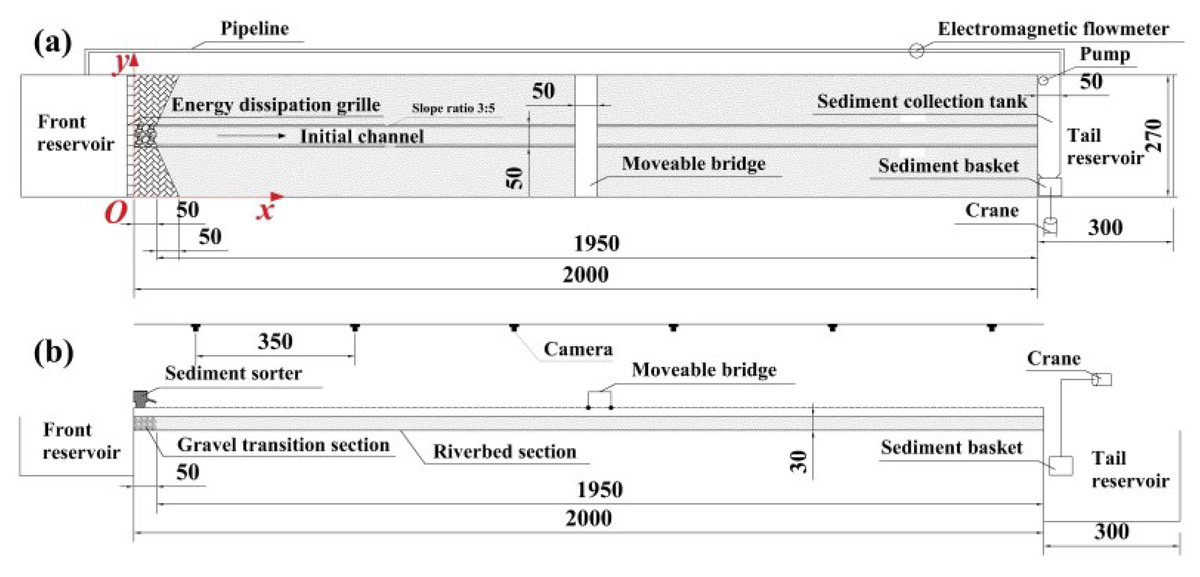
2. Experimental Arrangements

The experiments were conducted at the State Key Laboratory of Hydraulics and Mountain River Engineering, Sichuan University, using a 20 m long and 2.7 m wide flume with a 1.5% gradient. The flume is self-circulating, and the discharge is measured by a specially installed electromagnetic flowmeter. To ensure a smooth and controlled flow into the flume, a front reservoir is positioned upstream, followed by a 2 m gravel transition section. A tail reservoir is provided at the end of the flume to ensure self-circulation of the experiment flow. To accurately measure sediment transport, a sediment collection tank spanning the entire width of the flume is installed at the end of the flume. The sediment collection tank efficiently transports sediment from the outlet to a sediment basket, and a load cell provides real-time data on the amount of sediment delivered from the river section. In addition, a sediment sorter machine is placed at the inlet of the channel to supply sediment as required. A moveable bridge is equipped with a digital camera mount and the wood blade is positioned across the model sidewalls. Above the experimental flume, lights and cameras are placed for monitoring and recording changes in the channel planform over time. Control points are mounted on the inside of both sidewalls to allow Structure-from-Motion photogrammetry of the bed topography.
The schematic diagram of the modeling flume, shown in Figure 1, illustrates the established coordinate system. The coordinate system is defined with the origin at the point of contact between the bed surface and the upstream right sidewall of the flume. The x -axis pointing downwards is parallel to the flow, while the y -axis perpendicular to the sidewall is pointing towards the left bank, perpendicular to the flow direction. The z -axis pointing upwards is perpendicular to the coordinates.
The bed sediment of the flume was placed at a thickness of 0.3 m. The bed sediment composition was sand and gravel, and the bed grain size distribution is shown in Figure 2 where D10 = 0.293 mm, D50 = 0.904 mm, and D90 = 1.895 mm. In this work, four constant discharge experiments were carried out with discharge rates of 0.8 L/s, 1.3 L/s, 1.9 L/s, and 2.5 L/s. The experiments were divided into two phases: free evolution and experimental measurements. The experimental conditions are shown in Table 1.
At the beginning of each experiment, the bed of the flume was flattened using a large wood blade that spanned the width of the flume. A relatively small, straight initial channel was carved into the flat bed to concentrate the flow over the bed and speed up free evolution. During the experimental run, the sediment sorter rate at the upstream inlet was manually adjusted according to the load cell readings of sediment transport in the reach so that the upstream sediment supply was equal to downstream sediment transport to ensure that the channel was always in a state of equilibrium between erosion and deposition. The average wetted width and braiding intensity of the experimental reaches are used to determine whether the experimental channel has freely evolved from an initially straight channel to a braided channel with dynamic stability. It was observed that the time required for the free evolution of the channel is generally reduced as the stream power increases. During this time, the average wetted width and braiding intensity of the experimental channels were calculated by manual visual observation and recording, supplemented by photographs taken by cameras at the top of the flume. The time taken to develop from an initially straight channel to a dynamically stable braided channel for experiments 1–4 was 15 h, 15 h, 12 h, and 10 h. After the channel had reached dynamic stability, all four experiments underwent a 16 h measurement phase.
For each experiment, the 16 h of experimental runs were divided into 15 or 30 min intervals. Morphological methods, like those used here, are sensitive to the time interval between surveys, which must be long enough to allow for a detectable amount of morphological change but short enough that major changes in morphology are not compensated, resulting in no net vertical change. In light of this, preliminary experiments were conducted at corresponding discharge, and 15 min intervals were deemed appropriate for capturing images in the flume. However, experiment 1 necessitated an adjustment to 30 min intervals due to the limited morphological change observed within 15 min intervals, rendering it difficult to detect significant variations.
During each experiment run of either 15 or 30 min, six cameras positioned at the top of the flume diligently captured images of the channel morphology at 1 min intervals. Within the 2 min preceding the end of each experimental run, a digital camera affixed to the moveable bridge was employed to capture images of the wet surface. At the end of each experimental run, the flow within the model ceased, and the sediment in the downstream sediment basket was weighed. The flume was then left to drain until there was no obvious standing water in the deepest scour holes. A digital camera mounted on the moveable bridge was used to capture images of the dry surface. Two dry bed photo surveys were taken of each dry surface before moving on to the next experimental run.

3. Calculation Methods

3.1. Data Collection and Processing

There were six cameras installed at the top of the flume. Each camera covered an area of 4.5 m × 3.5 m, and there was an overlap of about 1 m between adjacent cameras. By setting up the cameras, all six cameras simultaneously captured images of the river channel morphology at 1 min intervals. These photographs were used to record the continuous evolution of the channel planform and to facilitate the calculation of wetted width and braiding intensity. Although the photos taken by these cameras were slightly different, these differences were corrected in post-processing using Adobe Photoshop. Adobe Photoshop was used for lens correction, cropping, and final image stitching.
In order to reduce the influence of the upstream water inlet and downstream water outlet of the model, a river section with a total length of 15 m from x = 3.5 18.5   m was selected as the research area for the experiments; at the same time, in order to eliminate the influence of the sidewalls of the flume, the above research area was cropped and finally selected the range of x = 3.5 18.5   m and y = 0.1 2.6   m as the research area of the experiment. The software package Agisoft PhotoScan Professional 1.7.5.13229 was used for photogrammetric processing to convert both the dry and wet bed photo surveys into high-resolution Digital Elevation Models (DEMs) and to generate orthophotos with 0.6 mm pixels, which is similar to the D50 of the model at 0.904 mm.
Orthophotos of the wetted surface were digitized using AutoCAD to quantify average braiding intensity, which represents the average number of wetted channels based on 1 m cross-section counts, and wetted width, calculated as the total area of water in channels divided by reach length. Given the large number of experimental runs, only a small subset of orthophotos was digitized for each experiment. For Experiment 1, only 8 orthophotos were digitized every two hours of experimental time. For Experiments 2–4, one orthophoto was digitized every hour of experimental time, evenly spaced out throughout the experiment. The DEMs of Difference (DoD), produced by subtracting successive DEMs, were used to quantitatively assess the temporal variations in the topography. Different thresholds corresponding to different experimental conditions were established to identify whether there were topographic changes, and these thresholds were subsequently applied to the original DoDs to calculate the parameters associated with each morphological change. If any absolute z values were below the threshold, these regions were considered to be unchanged and removed from the analysis. The corresponding thresholds for four constant discharge experiments are shown in Table 1.

3.2. Morphological Parameters

The total active area, defined as all areas of the flume that had topographic (i.e., morphological) change, were quantified in the DoDs as the sum of all erosion and deposition cells multiplied by the cell size. The reach-averaged morphological active width was estimated for each experimental run by dividing the total active area by the reach (i.e., 15 m) length:
a c t i v e   w i d t h = a c t i v e   a r e a r e a c h   l e n g t h
By multiplying the elevations (sum of z values) in the active areas of deposition and active areas of erosion by the cell size, it was possible to calculate the volume of deposition and erosion. The summed volumes of erosion represent all of the sediment moving from storage (i.e., eroding banks or bars), while the summed volumes of deposition represent additions to sediment storage (i.e., aggradation of bars). The total volume of morphological change, also known as the bulk change, was then calculated for each experimental run:
b u l k   c h a n g e = d e p o s i t i o n   v o l u m e + s c o u r   v o l u m e
The reach-averaged morphological active depth was estimated by dividing the total bulk change by the total active area for each experimental run:
a c t i v e   d e p t h = b u l k   c h a n g e a c t i v e   a r e a
The thresholds were applied to the original DoDs. The values between the thresholds are regarded as 0; therefore, any change in elevation ( z value) greater than 0 represented depositional areas, and less than 0 represented erosional areas. In this way, active area and bulk change, as well as active width and active depth, could be calculated from their separate erosional and depositional components for further analysis.
In order to compare and analyze the experimental data in different experimental conditions, it was necessary to calculate dimensionless stream power ( ω ) and dimensionless bedload transport rate ( q b ). The calculation methods were as follows:
ω = Q S b g Δ D 50 3
q b = Q S ρ b g Δ D 50 3
where Q is discharge, S is slope, D 50 is mean grain size, Δ is relative submerged density, b is the average wetted width, g is the acceleration due to gravity, Q S is bedload flux, and ρ is the water density.

3.3. Statistical Parameters

The statistical parameters primarily include variance ( σ 2 ), skewness ( S k ), and kurtosis ( K u ). These can be calculated according to Formulas (6)–(8):
σ 2 = 1 N i = 1 N ( z i z ¯ ) 2
S k = 1 N σ 3 i = 1 N ( z i z ¯ ) 3
K u = 1 N σ 4 i = 1 N ( z i z ¯ ) 4
where z i , z ¯ , and N represent the bed surface elevations, the sample mean, and the total sample number, respectively.
The variance reflects the degree of dispersion of the elevation samples relative to the sample mean. Skewness describes the symmetry of the elevation probability distribution, where S k > 0 is a positively skewed distribution, S k < 0 is a negatively skewed distribution, and S k = 0 is a symmetrical distribution. Kurtosis expresses the steepness of the elevation probability distribution, where K u = 3 is a normal distribution, K u > 3 is a leptokurtic distribution, and K u < 3 is a platykurtic distribution.

3.4. Variogram

A variogram, also known as the structure function, is a basic tool unique to geostatistics that can describe structural and random changes in regionalized variables. The variogram is usually defined as half the variance of the increments in two regionalized variable values, Z ( x ) and Z ( x + h ) , separated by | h | (representing the modulus of the vector) in either direction α (representing the direction of the vector h , i.e., the angle of the vector h with the x -axis), where x represents coordinate space, h represents vector space, and Z ( x ) and Z ( x + h ) are the values of the regionalized variables at spatial points x and x + h , respectively. The formula for calculating the two-dimensional variogram is
γ ( h ) = γ ( h x , h y ) = 1 2 ( M m ) ( N n ) i = 1 M m j = 1 N n [ z ( x i + m l x , y j + n l y ) z ( x i , y j ) ] 2
where γ ( h ) represents the variogram. x i and y j are the spatial point coordinates, respectively.
The above formula can be used to calculate the one-dimensional and two-dimensional structure function. In special cases, when h y = 0 but h x changes, or h x = 0 but h y changes, Formula (9) can be used to analyze the elevation variability in the x -axis and y -axis directions, respectively. The variability of the bed elevation can be reflected from different perspectives by the variation in the structure function and related parameters. In order to comprehensively understand the elevation variability of the entire study area, a number of variogram theoretical models have been proposed, among which the spherical model is the most commonly used, and its mathematical expression is
γ ( h ) = { 0 , h = 0 C 0 + C ( 3 2 h a 1 2 h 3 a 3 ) , 0 < h a C 0 + C , h > a
where C 0 is the nugget variance, C is the structural variance, C 0 + C is the sill, and a is the correlation length. The physical meaning of each parameter is as follows:
  • The nugget variance C 0 reflects the magnitude of the randomness of the regionalized variables. Theoretically, when the sampling scale h = 0 , the value of γ ( h ) should be equal to 0. However, due to the presence of microstructural variations (i.e., internal variability that occurs at scales smaller than the sampling scale h ) and errors associated with sampling, measurement, and analysis, γ ( h ) 0 when two sampling points are very close, leading to the existence of a nugget variance.
  • The sill C 0 + C reflects the magnitude of the variability of the regionalized variables, indicating the intensity of the variation within the study area. The ratio of the nugget variance to the sill is defined as the nugget coefficient, denoted as R C = C 0 / ( C 0 + C ) , which represents the proportion of spatial variability caused by the random component to the total variability, indicating the strength of spatial variability. If R C < 25 % , it indicates strong spatial correlation of the variable; if 25 % R C 75 % , it indicates moderate spatial correlation; if R C > 75 % , it indicates weak spatial correlation. A larger R C suggests that the variability is mainly due to random factors.
  • The correlation length a reflects the extent of spatial autocorrelation of the regionalized variables and represents the point where the spatial correlation transitions from existence to non-existence. When the sampling scale h < a , there is spatial correlation and mutual influence between two points in space, with the influence decreasing as the distance between the points increases. When the sampling scale h a , there is no spatial correlation between the two points.
The spherical model, as shown in Figure 3, has the slope of the tangent of this model at the coordinate origin ( h = 0 ) is 3 C / 2 a , and the distance from the tangent to the value C is 2 a / 3 . In order to quantitatively describe the variable characteristics of the entire region and accurately reflect the pattern of variable changes, it is necessary to perform the optimal curve fitting of the spherical model based on the experimental variogram values to estimate the parameters of the spherical model, namely, the nugget variance, sill, and correlation length. When estimating the parameters of the spherical model, the curve model can be transformed into a linear model using an appropriate transformation method, as follows:
γ ( h ) = y
h = x 1
h 3 = x 2
C 0 = b 0
3 C 2 a = b 1
C 2 a 3 = b 2
By substituting Equations (11)–(16) into the mathematical expression of the spherical model Equation (10), it can be transformed into the following linear model:
y = b 0 + b 1 x 1 + b 2 x 2
Then, the variogram values are fitted using the least squares method or the multivariate linear weighted regression method to calculate the parameters b 0 , b 1 , and b 2 , and subsequently compute the three parameters C 0 , C , and a of the spherical model.

4. Results and Discussion

4.1. Morphological Parameters of Braided Rivers

For each experimental run of the four constant discharge experiments, the DEMs of Difference (DoD) between two consecutive DEMs were used to determine the active area and bulk change, as well as active width and active depth of erosion and deposition in the reach. Figure 4 shows the DoD at the end of each constant discharge experiment and shows that even with 30 min intervals, there was minimal topographic change observed in Experiment 1. Compared to Experiment 1, Experiment 2 did not show a significant increase in the range of topographic change. This can be attributed to the more apparent phenomenon of flow adhering to the sidewall in Experiment 2, resulting in less lateral migration of the flow. However, it is noteworthy that the scour depth of Experiment 2 exceeded that of Experiment 1. One reason for this is the increase in stream power, resulting in a greater sediment transport capacity. Experiments 3 and 4 showed a border range of topographic change compared to Experiment 1, indicating increased complexity with greater braiding and higher active braiding intensity. In addition, several regions showed two or more major active channels (i.e., channels actively conveying sediment) and more extensive and continuous areas of erosion and deposition. The following conclusions can be drawn from the figure: (1) the active area and the average morphological active width became greater as discharge increased; (2) the active area became more continuous and contiguous as areas of erosion and deposition expanded; (3) the maximum depth of the morphological active layer remained almost unchanged.

4.2. Relationship between Morphological Active Width, Stream Power, and Bedload Transport Rate

During the constant discharge experiments, the average morphological active width of the reach for each experimental run was calculated based on DoD in the previous subsection. The average wetted width of the reach was calculated from the digitized orthophoto of the wetted surface. The mass of sediment transported was measured directly by the load cell. As illustrated in Figure 5, there is a clear positive correlation between the average morphological active width and total stream power, albeit exhibiting temporal variability during each constant discharge experiment. Figure 6 also indicates a noticeable positive correlation between the sediment transport rate and stream power. Based on the analysis conducted in the preceding section, it can be inferred that the average active width is closely associated with changes in the area and volume of the reach. Therefore, it can be used as an index of channel planform changes. In addition, sediment transport is related to flow movement and bedform. Consequently, it is possible to establish a connection between sediment transport, active width, and stream power. Figure 7 demonstrated a significant positive relationship between the bedload transport rate and the average active width and stream power; this finding is significant. To some extent, it showed that the easily measured and obtained data of discharge, bed surface particle size, wetted width, and active width, which characterize changes in river morphology, can be used to predict the mass of sediment transport that is difficult to measure directly.

4.3. Elevation Probability Distribution and Statistical Parameters of the Bed Surface

The bed surface elevation is considered a random distribution field, organized in ascending order and grouped based on specific elevation intervals for frequency statistics. In the analysis of this section, for each constant discharge experiment, the bed elevation within the river channel study area was measured and calculated every 2 h, involving a total of 32 sets of bed elevation data. This analysis takes the bed elevation information at the last moment of each constant discharge experiment as an example, as shown in Figure 8. It can be seen from the figure that the bed elevation probability distribution of the constant discharge experiments is basically “thin and high” with a negatively skewed distribution, which shows that the bed elevation distribution is relatively concentrated, and the elevation values below the average bed surface are slightly dominant, which also means that the mean value of the bed elevation distribution is basically the same and close to zero. According to the analysis in the two previous subsections, the bedform at different times is inconsistent due to the inherent variability of braided rivers. In order to facilitate analysis and comparison, for each constant discharge experiment, the average value of eight groups of statistical roughness parameters is taken to represent the roughness characteristics of the bed surface under this discharge. As the flow intensity increases, the lateral instability of braided rivers causes the flow to no longer be concentrated in the erosion and deposition of a few channels; instead, it develops into more extensive and more continuous channels, which also keeps the scour depth of the channel not getting bigger and bigger. Although the entire reach is in a state of erosion–deposition equilibrium, Figure 4 shows that the total erosion in the research reach is greater than deposition. This is due to the insufficient sediment transport capacity of the upstream reach, causing some sediment to deposit upstream. Specifically, the amount of upstream sediment supply was determined based on the downstream sediment transport, and thus, the upstream sediment supply had a certain hysteresis; in addition, the morphology of the river channel was constantly changing, which led to the fact that during the experimental run, the sediment transport capacity of the upstream flow could not always carry all the sediment supply at the inlet to the middle and downstream reaches, and thus, the upstream reach was occasionally slightly deposited, which mainly occurred in the range of x = 0–3 m. For the whole reach, the occasional deposition in the upstream does not affect the dynamic equilibrium state of the braided river, because when there is occasional slight deposition in the upstream, there is bound to be slight scouring in the middle and downstream reaches, which leads to the overall equilibrium state of the upstream sediment supply and the downstream sediment transport. However, for the research reach with changing bed topography (x = 3.5–18.5 m), slight deposition in the upstream inevitably leads to an overall scour greater than overall deposition in this research reach, which puts this research reach in a non-equilibrium state. It can be seen from Figure 9 that as the discharge increases, the overall variance of the bed surface elevation decreases, the overall negative skewness increases, the overall kurtosis changes little, and there is a relatively clear trend of correlation between skewness and the stream power. The relationship can be used as an index to characterize the topographic change in the bed surface.
Therefore, the relationship between the stream power and the bedload transport rate and the bed elevation skewness at the corresponding time is established here, and for the convenience of comparative analysis, the stream power and the bedload transport rate are dimensionless. Figure 10 shows that there is a relatively clear trend of correlation between the dimensionless stream power and the dimensionless bedload transport rate and skewness, but due to the complexity and inherent variability of braided rivers, the correlation coefficient is not sufficiently high. Therefore, as Figure 10c shows, the average values of the dimensionless bedload transport rate and skewness of different constant discharge experiments were analyzed, and it was found that there was a strong correlation between the two. To some extent, this means that the skewness based on the bed surface elevation can be used to estimate the bedload transport rate of braided rivers preliminarily.

4.4. Two-Dimensional Variograms of the Bed Surface Elevations

Based on the bed elevation data in the previous subsection, the two-dimensional variogram in geostatistics is used to analyze the riverbed area of the research reach. In order to facilitate analysis and comparison, the variance of the bed surface elevations is used to perform dimensionless processing on the two-dimensional variogram value, and the processed two-dimensional variogram is shown in Figure 11. It can be seen from the figure that the dimensionless two-dimensional variogram values are not the same in each direction, indicating that the bed elevation is anisotropic within the research reach. In addition, it can be found that the x -axis direction has less variability and is more stable than the y -axis direction. This can be attributed to the fact that the y -axis direction is perpendicular or intersects at a large angle to the flow direction. Bars are formed in braided rivers, and channel avulsion and bifurcation lead to the lateral movement of sediment, resulting in frequent changes in lateral erosion and deposition, and the lateral topography is complex and changeable. The bed surface elevation variogram in the x -axis direction is closer to the spherical model and only shows small fluctuations when the calculation scale is larger than the correlation length. Therefore, the spherical model can be an excellent theoretical model for quantifying its roughness properties.

4.5. One-Dimensional Variograms of the Bed Surface Elevations

Figure 12 shows the one-dimensional average variogram of the bed elevation in the x -axis direction, which is very consistent with the spherical model. As the discharge increases, the nugget variance, sill, and correlation length of the variogram all increase. At the same time, the nugget coefficient R C ranges from 0.112 to 0.184. It can be seen that R C < 25 % indicates that the bed elevation variable in the x -axis direction has a strong spatial correlation, and the bed surface elevation variation caused by random factors can be ignored. As flow intensity increases, the range of movement of the sediment on the bed surface expands and the randomness of the bed surface increases. The areas of erosion and deposition become more extensive and continuous, and the bed surface becomes more uneven and rougher, indicating that the sill and the correlation length can be used to characterize the bed surface roughness.
In order to make the analysis and comparison, the variance of the bed surface elevation is used to make the parameters of the spherical model dimensionless. It can be seen from Figure 13 that all three parameters increase with the increase in the dimensionless stream power, but the changing trend of the dimensionless nugget variance is not significant enough, and there is a relatively obvious relationship between the other two dimensionless parameters and the dimensionless stream power. However, the inherent variability and complexity of braided rivers lead to complex topographic changes, as reflected in the relatively scattered data points in the figure. In order to remove the influence of the inherent variability of braided rivers, this paper takes the average values of the relevant parameters for further analysis. It can be seen from Figure 14 that there is an obvious correlation between the average value of the three parameters of the spherical model and the dimensionless average stream power, but the correlation coefficient of the dimensionless nugget variance is only 0.64, whereas the other two parameters have correlation coefficients around 0.9, the correlation is very significant. In addition, it can be seen from Figure 15 that the correlation coefficients between the average value of the three parameters of the spherical model and the skewness are all above 0.9, and they all have very significant correlations. When the stream power increases, the movement time and distance of the sediment particles on the bed surface increase, so that the areas of erosion and deposition changes in the bed surface morphology increase. This leads to the occurrence of various phenomena such as channel bifurcation–confluence unit, bar formation, avulsion, and chute cutoff, which contribute to a more complex channel morphology. This process increases the variability of the bed surface elevation and enhances the spatial correlation of the elevation.
Based on the previous analysis, a clear correlation can be observed between the bedload transport rate, the stream power, skewness, and the parameters of the spherical model. In particular, the sill and correlation length have significant positive correlations with the stream power and skewness. Therefore, it can be tentatively assumed that there is a relationship between the variogram parameters and the bedload transport rate. Figure 16 demonstrates a significant positive correlation between the dimensionless sill, the dimensionless correlation length, and the dimensionless bedload transport rate, with correlation coefficients greater than 0.93. Therefore, the variogram parameters can be used to estimate the bedload transport rate in the reach.

5. Conclusions

This paper investigates the bed surface roughness properties of braided rivers by conducting four constant discharge experiments. It investigates the relationship between characteristic parameters of the channel planform morphology, bed surface elevation, and variogram parameters. The main conclusions are as follows:
  • The morphological change area of the reach becomes more continuous and extensive with increasing discharge. The average morphological active width increases, while the average morphological active depth remains almost unchanged.
  • There is a significant positive correlation between the bedload transport rate and the reach-averaged morphological active width and the stream power. This indicates that the easily measured parameters such as discharge, bed surface particle size, wetted width, and active width, which characterize morphological change, can be used to predict the mass of bedload transport that is difficult to measure directly.
  • The bed elevation probability distribution in braided rivers is negatively skewed and leptokurtic. There is a relatively significant correlation between skewness and the dimensionless bedload transport rate, providing a simple index for the preliminary prediction of bedload transport rate in braided rivers. The two-dimensional variogram values of the bed surface elevation differ in each direction, indicating anisotropy in bed surface roughness within the research reach.
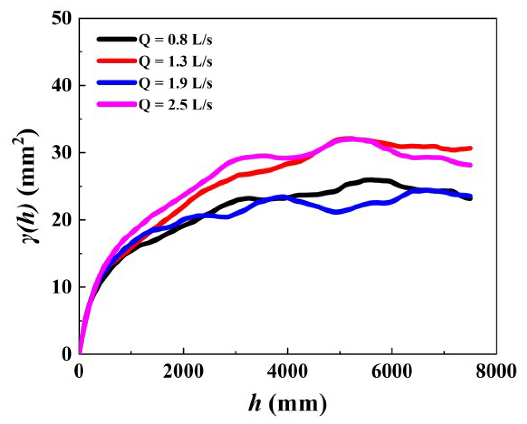
  • As flow intensity increases, bed surface roughness, the corresponding sill, and correlation length increase. The bed elevation variable in the x -axis direction has a strong spatial correlation, and elevation variation caused by random factors can be ignored. The sill and correlation length of the bed surface elevation variogram can be used to estimate the bedload transport rate in the constant discharge experiments of braided rivers.
  • This study primarily focused on different flow intensities. In the future, more extensive and systematic research should be conducted to analyze the influence of bed surface particle sizes, slopes, and different flow and sediment conditions on the statistical roughness properties of the bed surface in braided rivers to enrich the relevant research achievements.

Author Contributions

Conceptualization, B.R. and K.Y.; methodology, B.R. and Y.P.; software, B.R. and Y.P.; validation, B.R. and Y.P.; formal analysis, B.R.; investigation, B.R., Y.P. and X.L.; resources, B.R.; data curation, B.R.; writing—original draft preparation, B.R.; writing—review and editing, B.R. and K.Y.; visualization, B.R.; supervision, K.Y.; project administration, K.Y. All authors have read and agreed to the published version of the manuscript.

Funding

This work was financially supported by the National Key Research and Development Program of China (grant no. 2022YFE0128200) and the National Natural Science Foundation of China (grant no. 51979181).

Data Availability Statement

Not applicable.

Conflicts of Interest

The authors declare no conflict of interest.

References

  1. Surian, N. Fluvial processes in Braided Rivers. In Rivers—Physical, Fluvial and Environmental Processes; Rowiński, P., Radecki-Pawlik, A., Eds.; Springer: Cham, Switzerland, 2015; Chapter 15; pp. 403–425. [Google Scholar] [CrossRef]
  2. Leopold, L.B.; Wolman, M.G. River channel patterns-braided, meandering and straight. United States Geol. Surv. Prof. Paper 1957, 282A, 39–85. [Google Scholar]
  3. Bertoldi, W.; Zanoni, L.; Tubino, M. Planform dynamics of braided streams. Earth Surf. Process. Landf. 2009, 34, 547–557. [Google Scholar] [CrossRef]
  4. Ashmore, P. Morphology and Dynamics of Braided Rivers. In Treatise on Geomorphology; Shroder, J., Wohl, E., Eds.; Elsevier: San Diego, CA, USA, 2013; Volume 9, pp. 289–312. [Google Scholar] [CrossRef]
  5. Liu, C.; Shan, Y.Q. Impact of an emergent model vegetation patch on flow adjustment and velocity. Water Manag. 2022, 175, 55–66. [Google Scholar] [CrossRef]
  6. Yan, C.H.; Shan, Y.Q.; Liu, C.; Liu, X.N. Analytical model for predicting the lateral profiles of velocities through a partially vegetated channel. J. Hydrol. 2022, 612, 128137. [Google Scholar] [CrossRef]
  7. Liu, C.; Yan, C.H.; Sun, S.C.; Lei, J.R.; Nepf, H.; Shan, Y.Q. Velocity, turbulence, and sediment deposition in a channel partially filled with a Phragmites australis canopy. Water Resour. Res. 2022, 58, e2022WR032381. [Google Scholar] [CrossRef]
  8. Gui, Z.Q.; Shan, Y.Q.; Liu, C. Flow velocity evolution through a floating rigid cylinder array under unidirectional flow. J. Hydrol. 2023, 617, 128915. [Google Scholar] [CrossRef]
  9. Pender, G.; Hoey, T.B.; Fuller, C.; McEwan, I.K. Selective bedload transport during the degradation of a well sorted graded sediment bed. J. Hydraul. Res. 2001, 39, 269–277. [Google Scholar] [CrossRef]
  10. Haynes, H.; Pender, G. Stress history effects on graded bed stability. J. Hydraul. Eng. 2007, 133, 343–349. [Google Scholar] [CrossRef]
  11. Luo, M.; Wang, X.K.; Yan, X.F.; Huang, E. Applying the mixing layer analogy for flow resistance evaluation in gravel-bed streams. J. Hydrol. 2020, 589, 125119. [Google Scholar] [CrossRef]
  12. Fu, H.S.; Shan, Y.Q.; Liu, C. A model for predicting the grain size distribution of an armor layer under clear water scouring. J. Hydrol. 2023, 623, 129842. [Google Scholar] [CrossRef]
  13. Liu, C.; Nepf, H. Sediment deposition within and around a finite patch of model vegetation over a range of channel velocity. Water Resour. Res. 2016, 52, 600–612. [Google Scholar] [CrossRef] [Green Version]
  14. Ackers, P.; White, W. Sediment transport: New approach and analysis. J. Hydraul. Eng. 1973, 99, 2041–2060. [Google Scholar] [CrossRef]
  15. Kamphuis, J.W. Determination of sand roughness for fixed beds. J. Hydraul. Res. 1974, 12, 193–203. [Google Scholar] [CrossRef]
  16. Whiting, P.J.; Dietrich, W.E. Boundary shear-stress and roughness over mobile alluvial beds. J. Hydraul. Eng. 1990, 116, 1495–1511. [Google Scholar] [CrossRef]
  17. Powell, D.M. Flow resistance in gravel-bed rivers: Progress in research. Earth-Sci. Rev. 2014, 136, 301–338. [Google Scholar] [CrossRef]
  18. Robert, A. Statistical properties of sediment bed profiles in alluvial channels. Math. Geol. 1988, 20, 205–225. [Google Scholar] [CrossRef]
  19. Bertin, S.; Friedrich, H. Measurement of gravel-bed topography: Evaluation study applying statistical roughness analysis. J. Hydraul. Eng. 2014, 140, 269–279. [Google Scholar] [CrossRef]
  20. Wu, W.M.; Wang, S.S.Y.; Jia, Y.F. Nonuniform sediment transport in alluvial rivers. J. Hydraul. Res. 2000, 38, 427–434. [Google Scholar] [CrossRef]
  21. Bai, Y.C.; Wang, X.; Cao, Y.G. Incipient motion of non-uniform coarse grain of bedload considering the impact of two-way exposure. Sci. China Tech. Sci. 2013, 56, 1896–1905. [Google Scholar] [CrossRef]
  22. Xing, R.; Zhang, G.G.; Liang, Z.X.; Wu, Z.S. Study on the location characteristics of bed surface particle. J. Sediment Res. 2016, 4, 28–33. [Google Scholar] [CrossRef]
  23. Sapozhnikov, V.; Foufoula-Georgiou, E. Self-affinity in braided rivers. Water Resour. Res. 1996, 32, 1429–1439. [Google Scholar] [CrossRef]
  24. Robert, A. Fractal properties of simulated bed profiles in coarse-grained channels. Math. Geol. 1991, 23, 367–382. [Google Scholar] [CrossRef]
  25. Butler, J.B.; Lane, S.N.; Chandler, J.H. Characterization of the structure of riverbed gravels using two-dimensional fractal analysis. Math. Geol. 2001, 33, 301–330. [Google Scholar] [CrossRef]
  26. Papanicolaou, A.N.; Tsakiris, A.G.; Strom, K.B. The use of fractals to quantify the morphology of cluster microforms. Geomorphology 2012, 139, 91–108. [Google Scholar] [CrossRef]
  27. Aubeneau, A.F.; Martin, R.L.; Bolster, D.; Schumer, R.; Jerolmack, D.; Packman, A. Fractal patterns in riverbed morphology produce fractal scaling of water storage times. Geophys. Res. Lett. 2015, 42, 5309–5315. [Google Scholar] [CrossRef] [Green Version]
  28. Brasington, J.; Vericat, D.; Rychkov, I. Modeling river bed morphology, roughness, and surface sedimentology using high resolution terrestrial laser scanning. Water Resour. Res. 2012, 48, W11519. [Google Scholar] [CrossRef] [Green Version]
  29. Bouratsis, P.P.; Diplas, P.; Dancey, C.L.; Apsilidis, N. High-resolution 3-D monitoring of evolving sediment beds. Water Resour. Res. 2013, 49, 977–992. [Google Scholar] [CrossRef] [Green Version]
  30. Morgan, J.A.; Brogan, D.J.; Nelson, P.A. Application of Structure-from-Motion photogrammetry in laboratory flumes. Geomorphology 2017, 276, 125–143. [Google Scholar] [CrossRef]
  31. Nikora, V.I.; Goring, D.G.; Biggs, B.J.F. On gravel-bed roughness characterization. Water Resour. Res. 1998, 34, 517–527. [Google Scholar] [CrossRef]
  32. Nikora, V.; Walsh, J. Water-worked gravel surfaces: High-order structure functions at the particle scale. Water Resour. Res. 2004, 40, W12601. [Google Scholar] [CrossRef]
  33. Aberle, J.; Nikora, V. Statistical properties of armored gravel bed surfaces. Water Resour. Res. 2006, 42, W11414. [Google Scholar] [CrossRef]
  34. Aberle, J.; Nikora, V.; Henning, M.; Ettmer, B.; Hentschel, B. Statistical characterization of bed roughness due to bed forms: A field study in the Elbe River at Aken, Germany. Water Resour. Res. 2010, 46, W03521. [Google Scholar] [CrossRef]
  35. Pan, Y.W.; Liu, X.; Cai, T.; Yang, K.J. Influences of average particle size and non-uniformity on the statistical roughness characteristics of gravel-bed surfaces. Arab. J. Geosci. 2022, 15, 1021. [Google Scholar] [CrossRef]
  36. Pan, Y.W.; Xia, J.Q.; Yang, K.J. Statistical roughness properties of the gravel bed surfaces in a meandering channel. J. Hydrol. 2023, 617, 128966. [Google Scholar] [CrossRef]
  37. Egozi, R.; Ashmore, P. Defining and measuring braiding intensity. Earth Surf. Process. Landf. 2008, 33, 2121–2138. [Google Scholar] [CrossRef]
  38. Sarma, J.N.; Acharjee, S. A study on variation in channel width and braiding intensity of the Brahmaputra River in Assam, India. Geosciences 2018, 8, 343. [Google Scholar] [CrossRef] [Green Version]
  39. Das, B.C.; Islam, A. Reviewing braiding indices of the river channel in an attempt to establish alternatives. MethodsX 2023, 10, 102042. [Google Scholar] [CrossRef]
Figure 1. Schematic of the river modeling flume. (a) plan view; (b) side view. (Note: the unit in the figure is cm.)
Water 15 02612 g001
Figure 2. Grain size distribution of the flume.
Water 15 02612 g002
Figure 3. Spherical model of variogram.
Water 15 02612 g003
Figure 4. DEMs of difference generated using the final two DEMs from the four constant discharge experiments. Flow was from left to right. (a) Run 1: Q = 0.8 L/s. (b) Run 2: Q = 1.3 L/s. (c) Run 3: Q = 1.9 L/s. (d) Run 4: Q = 2.5 L/s.
Water 15 02612 g004
Figure 5. Reach-averaged morphological active width as a function of (a) total stream power (Ω) and (b) experimental run time for the constant discharge experiments.
Water 15 02612 g005
Figure 6. Bedload transport rates for each total stream power of the constant discharge experiments.
Water 15 02612 g006
Figure 7. (a) Bedload transport rate plotted against reach-averaged morphological active width; (b) dimensionless bedload transport rate plotted against dimensionless stream power for constant discharge experiments. The dashed line represents the linear regression through all observations.
Water 15 02612 g007
Figure 8. Elevation probability distribution of the bed surface. (a) Run 1: Q = 0.8 L/s. (b) Run 2: Q = 1.3 L/s. (c) Run 3: Q = 1.9 L/s. (d) Run 4: Q = 2.5 L/s.
Water 15 02612 g008
Figure 9. Average statistical roughness parameters as a function of discharge for the constant discharge experiments. (a) Variance σ 2 ; (b) skewness S k ; (c) kurtosis K u . The dashed line represents the linear regression through all observations.
Water 15 02612 g009
Figure 10. Dimensionless stream power and dimensionless bedload transport rate plotted against skewness for the constant discharge experiments. (a) The variation in ω with S k ; (b) the variation in q b with S k ; (c) the variation in average q b with average S k . The dashed line represents the linear regression through all observations.
Water 15 02612 g010
Figure 11. Two-dimensional variograms of the bed surface elevations. (a) Run 1: Q = 0.8 L/s. (b) Run 2: Q = 1.3 L/s. (c) Run 3: Q = 1.9 L/s. (d) Run 4: Q = 2.5 L/s.
Water 15 02612 g011
Figure 12. One-dimensional average variograms of the bed surface elevations.
Water 15 02612 g012
Figure 13. Spherical model parameters of the variograms plotted against dimensionless stream power. (a) The variation in C 0 / σ 2 with ω ; (b) the variation in ( C 0 + C ) / σ 2 with ω ; (c) the variation in a / σ 2 with ω . The dashed line represents the linear regression through all observations.
Water 15 02612 g013
Figure 14. Average spherical model parameters of the variograms plotted against average dimensionless stream power. (a) The variation in average C 0 / σ 2 with average ω ; (b) the variation in average ( C 0 + C ) / σ 2 with average ω ; (c) the variation in average a / σ 2 with average ω . The dashed line represents the linear regression through all observations.
Water 15 02612 g014
Figure 15. Average spherical model parameters of the variograms plotted against average skewness. (a) The variation in average C 0 / σ 2 with average S k ; (b) the variation in average ( C 0 + C ) / σ 2 with average S k ; (c) the variation in average a / σ 2 with average S k . The dashed line represents the linear regression through all observations.
Water 15 02612 g015
Figure 16. Average spherical model parameters of the variograms plotted against average dimensionless bedload transport rate. (a) The variation in average C 0 / σ 2 with average q b ; (b) the variation in average ( C 0 + C ) / σ 2 with average q b ; (c) the variation in average a / σ 2 with average q b . The dashed line represents the linear regression through all observations.
Water 15 02612 g016
Table 1. Summary of the experimental conditions.
ExperimentSlopeDischargeStream PowerEvolution TimeExperimental Run TimeThreshold
SQΩ
(%)(L/s)(W/m)(h)(h)(mm)
Run 11.50.80.1215162.42
Run 21.51.30.1915162.18
Run 31.51.90.2812161.98
Run 41.52.50.3710161.70
Disclaimer/Publisher’s Note: The statements, opinions and data contained in all publications are solely those of the individual author(s) and contributor(s) and not of MDPI and/or the editor(s). MDPI and/or the editor(s) disclaim responsibility for any injury to people or property resulting from any ideas, methods, instructions or products referred to in the content.

