
Comparative Assessment of Sap Flow Modeling Techniques in European Beech Trees: Can Linear Models Compete with Random Forest, Extreme Gradient Boosting, and Neural Networks?

 ,
,  , and
, and 
Abstract
1. Introduction
2. Materials and Methods
2.1. Study Site
2.2. Sap Flow Measurements
2.3. Monitoring of Environmental Conditions
2.4. Model Development and Machine Learning
3. Results and Discussion
4. Conclusions
Author Contributions
Funding
Data Availability Statement
Acknowledgments
Conflicts of Interest
References
- Mukarram, M.; Choudhary, S.; Kurjak, D.; Petek, A.; Khan, M.M.A. Drought: Sensing, Signalling, Effects and Tolerance in Higher Plants. Physiol. Plant. 2021, 172, 1291–1300. [Google Scholar] [CrossRef] [PubMed]
- Oogathoo, S.; Houle, D.; Duchesne, L.; Kneeshaw, D. Vapour Pressure Deficit and Solar Radiation Are the Major Drivers of Transpiration of Balsam Fir and Black Spruce Tree Species in Humid Boreal Regions, Even during a Short-Term Drought. Agric. For. Meteorol. 2020, 291, 108063. [Google Scholar] [CrossRef]
- Schlesinger, W.H.; Jasechko, S. Transpiration in the Global Water Cycle. Agric. For. Meteorol. 2014, 189, 115–117. [Google Scholar] [CrossRef]
- Eamus, D.; Boulain, N.; Cleverly, J.; Breshears, D.D. Global Change-Type Drought-Induced Tree Mortality: Vapor Pressure Deficit Is More Important than Temperature per Se in Causing Decline in Tree Health. Ecol. Evol. 2013, 3, 2711–2729. [Google Scholar] [CrossRef] [PubMed]
- Lüttschwager, D.; Jochheim, H. Drought Primarily Reduces Canopy Transpiration of Exposed Beech Trees and Decreases the Share of Water Uptake from Deeper Soil Layers. Forests 2020, 11, 537. [Google Scholar] [CrossRef]
- Zavadilová, I.; Szatniewska, J.; Petrík, P.; Mauer, O.; Pokornỳ, R.; Stojanović, M. Sap Flow and Growth Response of Norway Spruce under Long-Term Partial Rainfall Exclusion at Low Altitude. Front. Plant Sci. 2023, 14, 1089706. [Google Scholar] [CrossRef]
- Xing, L.; Cui, N.; Liu, C.; Zhao, L.; Guo, L.; Du, T.; Zhan, C.; Wu, Z.; Wen, S.; Jiang, S. Estimation of Daily Apple Tree Transpiration in the Loess Plateau Region of China Using Deep Learning Models. Agric. Water Manag. 2022, 273, 107889. [Google Scholar] [CrossRef]
- Fan, J.; Zheng, J.; Wu, L.; Zhang, F. Estimation of Daily Maize Transpiration Using Support Vector Machines, Extreme Gradient Boosting, Artificial and Deep Neural Networks Models. Agric. Water Manag. 2021, 245, 106547. [Google Scholar] [CrossRef]
- Wang, H.; Guan, H.; Simmons, C.T. Modeling the Environmental Controls on Tree Water Use at Different Temporal Scales. Agric. For. Meteorol. 2016, 225, 24–35. [Google Scholar] [CrossRef]
- Fan, J.; Yue, W.; Wu, L.; Zhang, F.; Cai, H.; Wang, X.; Lu, X.; Xiang, Y. Evaluation of SVM, ELM and Four Tree-Based Ensemble Models for Predicting Daily Reference Evapotranspiration Using Limited Meteorological Data in Different Climates of China. Agric. For. Meteorol. 2018, 263, 225–241. [Google Scholar] [CrossRef]
- Zlatník, A. Overview of Groups of Types of Geobiocoenes Originally Forest and Shrubby. Zprávy Geogr. Čsav Brno 1976, 13, 55–56. [Google Scholar]
- Sitková, Z.; Strelcová, K.; Jezík, M.; Sitko, R.; Pavlenda, P.; Hlásny, T. How Does Soil Water Potential Limit the Seasonal Dynamics of Sap Flow and Circumference Changes in European Beech? Lesn. Cas. 2014, 60, 19. [Google Scholar] [CrossRef]
- Čermák, J.; Kučera, J.; Nadezhdina, N. Sap Flow Measurements with Some Thermodynamic Methods, Flow Integration within Trees and Scaling up from Sample Trees to Entire Forest Stands. Trees 2004, 18, 529–546. [Google Scholar] [CrossRef]
- Kučera, J.; Čermák, J.; Penka, M. Improved Thermal Method of Continual Recording the Transpiration Flow Rate Dynamics. Biol Plant 1977, 19, 413–420. [Google Scholar] [CrossRef]
- Nalevanková, P.; Sitková, Z.; Kučera, J.; Střelcová, K. Impact of Water Deficit on Seasonal and Diurnal Dynamics of European Beech Transpiration and Time-Lag Effect between Stand Transpiration and Environmental Drivers. Water 2020, 12, 3437. [Google Scholar] [CrossRef]
- Penman, H.L.; Keen, B.A. Natural Evaporation from Open Water, Bare Soil and Grass. Proc. R. Soc. London. Ser. A. Math. Phys. Sci. 1948, 193, 120–145. [Google Scholar] [CrossRef]
- James, G.; Witten, D.; Hastie, T.; Tibshirani, R. An Introduction to Statistical Learning; Springer: Berlin/Heidelberg, Germany, 2013; Volume 112. [Google Scholar]
- Leštianska, A.; Fleischer, P.; Merganičová, K.; Fleischer, P.; Nalevanková, P.; Střelcová, K. Effect of Provenance and Environmental Factors on Tree Growth and Tree Water Status of Norway Spruce. Forests 2023, 14, 156. [Google Scholar] [CrossRef]
- Shavitt, I.; Segal, E. Regularization Learning Networks: Deep Learning for Tabular Datasets. In Proceedings of the Advances in Neural Information Processing Systems; Curran Associates, Inc.: Red Hook, NY, USA, 2018; Volume 31. [Google Scholar]
- Sagawa, S.; Koh, P.W.; Hashimoto, T.B.; Liang, P. Distributionally Robust Neural Networks for Group Shifts: On the Importance of Regularization for Worst-Case Generalization. arXiv 2019, arXiv:1911.08731. [Google Scholar]
- Hayat, M.; Zha, T.; Jia, X.; Iqbal, S.; Qian, D.; Bourque, C.P.-A.; Khan, A.; Tian, Y.; Bai, Y.; Liu, P.; et al. A Multiple-Temporal Scale Analysis of Biophysical Control of Sap Flow in Salix Psammophila Growing in a Semiarid Shrubland Ecosystem of Northwest China. Agric. For. Meteorol. 2020, 288–289, 107985. [Google Scholar] [CrossRef]
- Zhang, R.; Xu, X.; Liu, M.; Zhang, Y.; Xu, C.; Yi, R.; Luo, W.; Soulsby, C. Hysteresis in Sap Flow and Its Controlling Mechanisms for a Deciduous Broad-Leaved Tree Species in a Humid Karst Region. Sci. China Earth Sci. 2019, 62, 1744–1755. [Google Scholar] [CrossRef]
- Li, Y.; Ye, J.; Xu, D.; Zhou, G.; Feng, H. Prediction of Sap Flow with Historical Environmental Factors Based on Deep Learning Technology. Comput. Electron. Agric. 2022, 202, 107400. [Google Scholar] [CrossRef]
- Wu, Z.; Cui, N.; Gong, D.; Zhu, F.; Xing, L.; Zhu, B.; Chen, X.; Wen, S.; Liu, Q. Simulation of Daily Maize Evapotranspiration at Different Growth Stages Using Four Machine Learning Models in Semi-Humid Regions of Northwest China. J. Hydrol. 2023, 617, 128947. [Google Scholar] [CrossRef]
- Amir, A.; Butt, M.; Van Kooten, O. Using Machine Learning Algorithms to Forecast the Sap Flow of Cherry Tomatoes in a Greenhouse. IEEE Access. 2021, 9, 154183–154193. [Google Scholar] [CrossRef]
- Tu, J.; Liu, Q.; Wu, J. Recognition of Dominant Driving Factors behind Sap Flow of Liquidambar Formosana Based on Back-Propagation Neural Network Method. Ann. Forest Sci. 2021, 78, 95. [Google Scholar] [CrossRef]
- Liu, X.; Kang, S.; Li, F. Simulation of Artificial Neural Network Model for Trunk Sap Flow of Pyrus Pyrifolia and Its Comparison with Multiple-Linear Regression. Agric. Water Manag. 2009, 96, 939–945. [Google Scholar] [CrossRef]
- Tu, J.; Wei, X.; Huang, B.; Fan, H.; Jian, M.; Li, W. Improvement of Sap Flow Estimation by Including Phenological Index and Time-Lag Effect in Back-Propagation Neural Network Models. Agric. Forest Meteorol. 2019, 276–277, 107608. [Google Scholar] [CrossRef]


| Variants | Data Manipulation and Filtering | ||||
|---|---|---|---|---|---|
| Rs Shifted 1 h | Rs above 200 W m−2 | SWP Values | Data Size n | Sum of Sap Flow (kg cm−1) | |
| Variant 1 | - | - | from 0 to −1.45 MPa | 10318 | 192.2 |
| Variant 2 | yes | - | from 0 to −1.45 MPa | 10318 | 192.2 |
| Variant 3 | yes | - | from −0.8 to −1.45 MPa (drier soil conditions) | 3323 | 58.7 |
| Variant 4 | yes | yes | from −0.8 to −1.45 MPa (drier soil conditions) | 1158 | 22.0 |
| Variant 5 | yes | yes | from 0 to −0.4 MPa (wetter soil conditions) | 2332 | 50.1 |
| Variant 6 | - | yes | from 0 to −1.45 MPa | 3488 | 160.3 |
| Variant 1 | Method | ||||||
| NN | RF | XGBM | LM | ||||
| model description | n | 10318 | RMSE | 0.007 | 0.006 | 0.005 | 0.014 |
| all available data used | real SF | 192.2 | R2 | 0.937 | 0.954 | 0.970 | 0.764 |
| Rs non-shifted | MAD | 0.002 | 0.001 | 0.001 | 0.005 | ||
| pred. SF | 211.0 | 192.8 | 192.9 | 194.8 | |||
| pred. SF/SF | 1.1 | 1.0 | 1.0 | 1.0 | |||
| Variant 2 | Method | ||||||
| NN | RF | XGBM | LM | ||||
| model description | n | 10318 | RMSE | 0.010 | 0.006 | 0.005 | 0.014 |
| all available data used | real SF | 192.2 | R2 | 0.894 | 0.961 | 0.973 | 0.762 |
| Rs 1 h shifted | MAD | 0.005 | 0.001 | 0.001 | 0.006 | ||
| pred. SF | 253.6 | 194.9 | 194.7 | 193.2 | |||
| pred. SF/SF | 1.3 | 1.0 | 1.0 | 1.0 | |||
| Variant 3 | Method | ||||||
| NN | RF | XGBM | LM | ||||
| model description | n | 3323 | RMSE | 0.008 | 0.005 | 0.005 | 0.013 |
| SWP below −0.8 MPa | real SF | 58.7 | R2 | 0.887 | 0.954 | 0.960 | 0.713 |
| Rs 1 h shifted | MAD | 0.004 | 0.001 | 0.001 | 0.007 | ||
| pred. SF | 59.0 | 58.5 | 58.2 | 59.2 | |||
| pred. SF/SF | 1.0 | 1.0 | 1.0 | 1.0 | |||
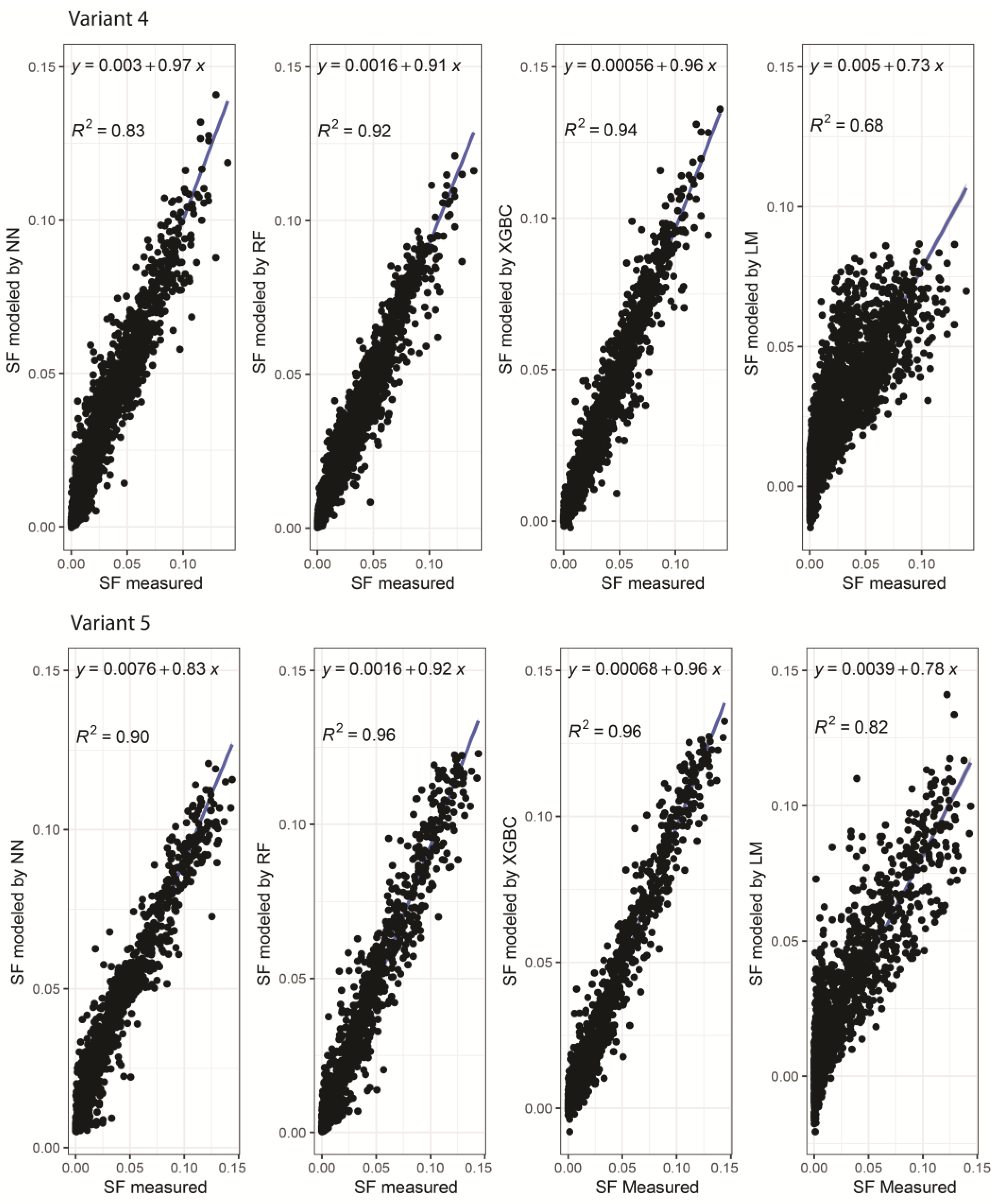
| Variant 4 | Method | ||||||
| NN | RF | XGBM | LM | ||||
| model description | n | 1158 | RMSE | 0.010 | 0.007 | 0.006 | 0.014 |
| SWP below −0.8 Mpa | real SF | 22.0 | R2 | 0.834 | 0.917 | 0.937 | 0.683 |
| Rs > 200 W m−2 | MAD | 0.008 | 0.002 | 0.002 | 0.008 | ||
| Rs 1 h shifted | pred. SF | 21.0 | 22.1 | 22.2 | 22.1 | ||
| pred. SF/SF | 1.0 | 1.0 | 1.0 | 1.0 | |||
| Variant 5 | Method | ||||||
| NN | RF | XGBM | LM | ||||
| model description | n | 2332 | RMSE | 0.010 | 0.007 | 0.006 | 0.014 |
| SWP above −0.4 Mpa | real SF | 50.1 | R2 | 0.901 | 0.956 | 0.963 | 0.815 |
| Rs > 200 W m−2 | MAD | 0.006 | 0.002 | 0.001 | 0.006 | ||
| Rs 1 h shifted | pred. SF | 59.2 | 49.7 | 49.8 | 49.7 | ||
| pred. SF/SF | 1.2 | 1.0 | 1.0 | 1.0 | |||
| Variant 6 | Method | ||||||
| NN | RF | XGBM | LM | ||||
| model description | n | 3488 | RMSE | 0.018 | 0.009 | 0.007 | 0.021 |
| Rs > 200 W m−2 | real SF | 160.3 | R2 | 0.709 | 0.922 | 0.954 | 0.626 |
| Rs non-shifted | MAD | 0.015 | 0.005 | 0.004 | 0.014 | ||
| pred. SF | 207.4 | 160.5 | 160.7 | 162.7 | |||
| pred. SF/SF | 1.3 | 1.0 | 1.0 | 1.0 | |||
Disclaimer/Publisher’s Note: The statements, opinions and data contained in all publications are solely those of the individual author(s) and contributor(s) and not of MDPI and/or the editor(s). MDPI and/or the editor(s) disclaim responsibility for any injury to people or property resulting from any ideas, methods, instructions or products referred to in the content. |
© 2023 by the authors. Licensee MDPI, Basel, Switzerland. This article is an open access article distributed under the terms and conditions of the Creative Commons Attribution (CC BY) license (https://creativecommons.org/licenses/by/4.0/).
Share and Cite
Nalevanková, P.; Fleischer, P., Jr.; Mukarram, M.; Sitková, Z.; Střelcová, K. Comparative Assessment of Sap Flow Modeling Techniques in European Beech Trees: Can Linear Models Compete with Random Forest, Extreme Gradient Boosting, and Neural Networks? Water 2023, 15, 2525. https://doi.org/10.3390/w15142525
Nalevanková P, Fleischer P Jr., Mukarram M, Sitková Z, Střelcová K. Comparative Assessment of Sap Flow Modeling Techniques in European Beech Trees: Can Linear Models Compete with Random Forest, Extreme Gradient Boosting, and Neural Networks? Water. 2023; 15(14):2525. https://doi.org/10.3390/w15142525
Chicago/Turabian StyleNalevanková, Paulína, Peter Fleischer, Jr., Mohammad Mukarram, Zuzana Sitková, and Katarína Střelcová. 2023. "Comparative Assessment of Sap Flow Modeling Techniques in European Beech Trees: Can Linear Models Compete with Random Forest, Extreme Gradient Boosting, and Neural Networks?" Water 15, no. 14: 2525. https://doi.org/10.3390/w15142525
APA StyleNalevanková, P., Fleischer, P., Jr., Mukarram, M., Sitková, Z., & Střelcová, K. (2023). Comparative Assessment of Sap Flow Modeling Techniques in European Beech Trees: Can Linear Models Compete with Random Forest, Extreme Gradient Boosting, and Neural Networks? Water, 15(14), 2525. https://doi.org/10.3390/w15142525