
Stochastic Assessment of Scour Hazard


Abstract
1. Introduction
2. Data Processing
2.1. Preprocessing
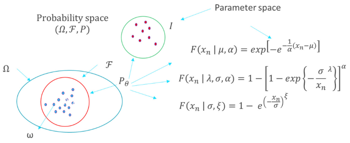
2.2. Statistical Inference of
2.3. Missing Data Inference
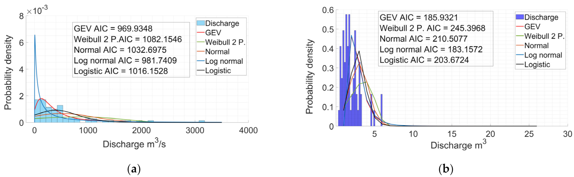
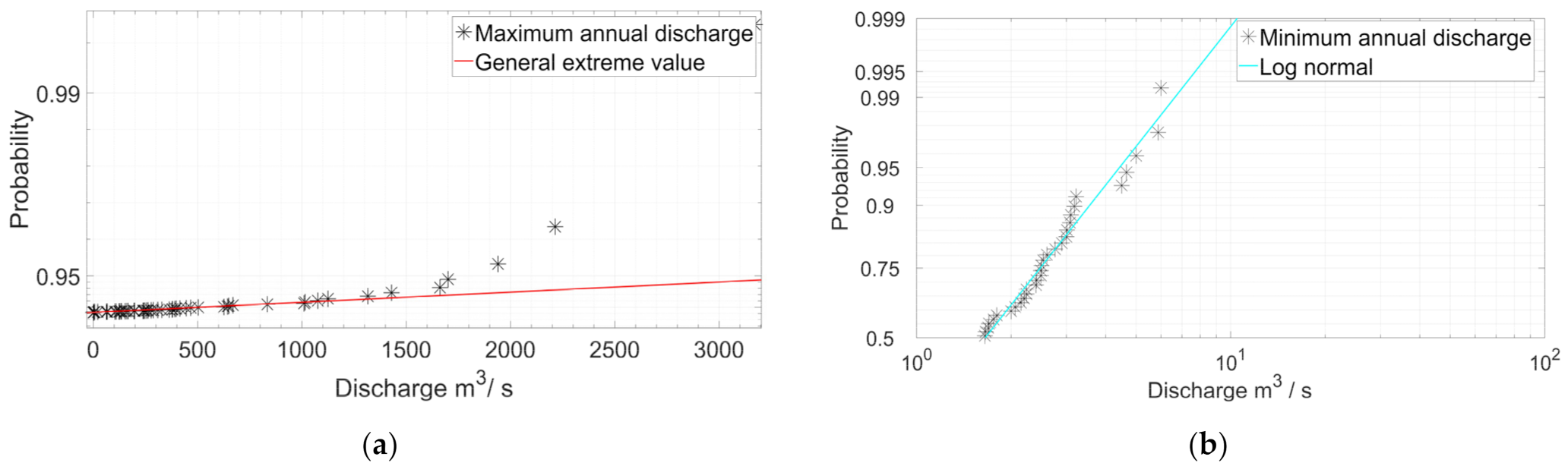
2.4. Suitable Probability Distribution
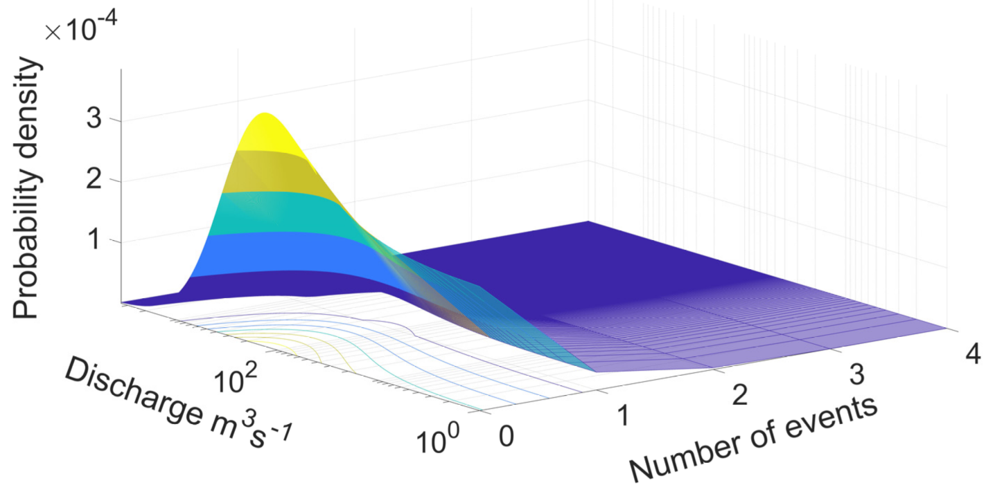
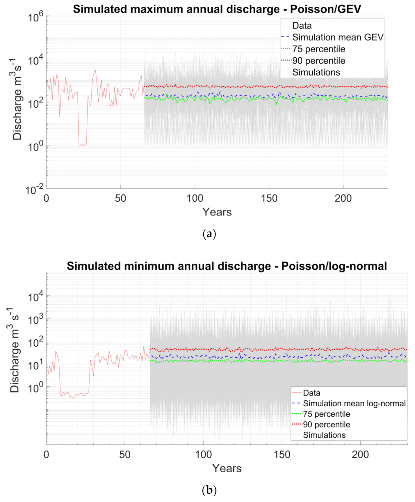
2.5. Simulation of Events for the Proposed Approach
2.6. Simulation of Time Series for SRICOS-EFA Method
3. Scour and Fill
3.1. Scour
3.2. Fill
4. Scour Hazard Curves
4.1. Simulation of Random Events
4.2. Hazard Curves
5. Case Study
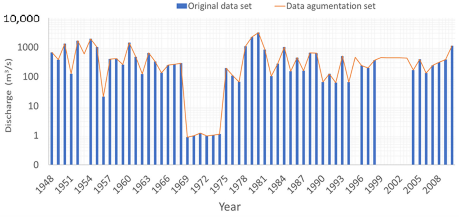
5.1. Data Augmentation
5.2. Fit to a Probability Distribution
5.3. Simulation of Events
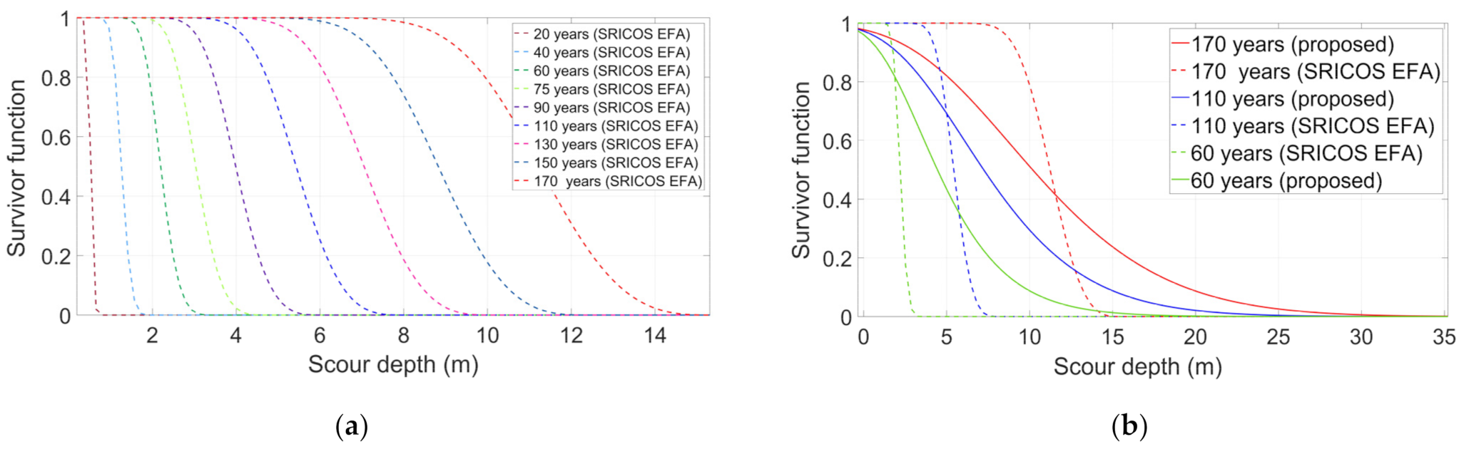
5.4. Scour Survival Function
5.5. Discussion
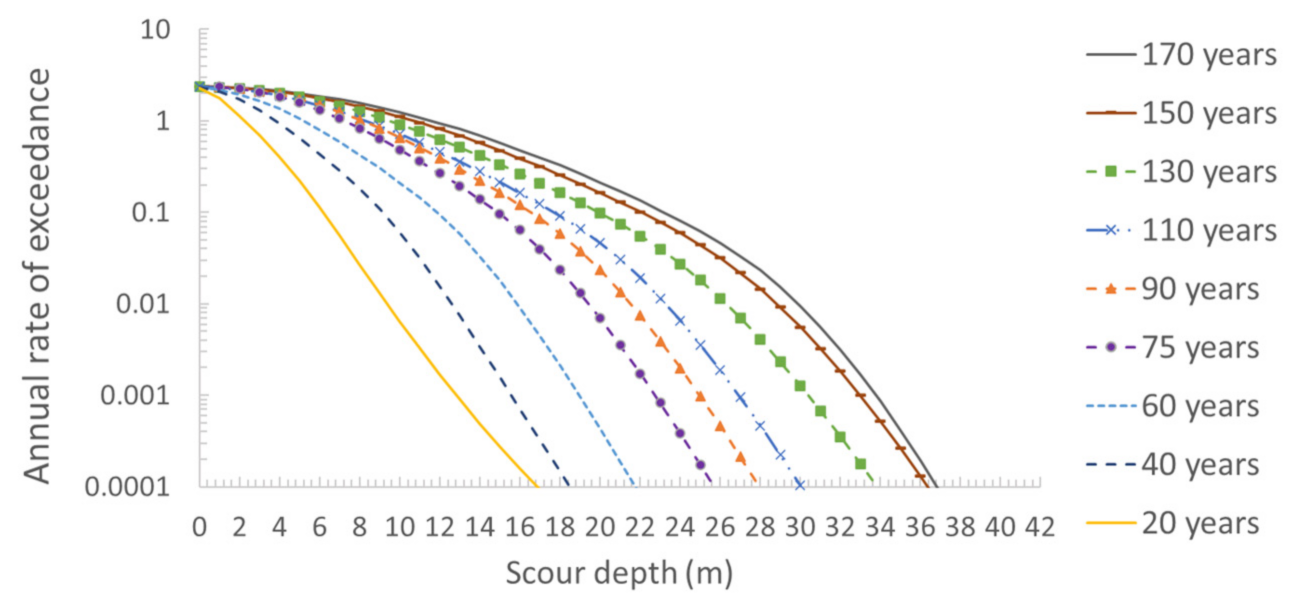
5.6. Scour Hazard
6. Concluding Remarks
Author Contributions
Funding
Institutional Review Board Statement
Informed Consent Statement
Data Availability Statement
Acknowledgments
Conflicts of Interest
References
- Pizarro, A.; Manfreda, S.; Tubaldi, E. The science behind scour at bridge foundations: A review. Water 2020, 12, 374. [Google Scholar] [CrossRef]
- Mahalder, B.; Schwartz, J.S.; Palomino, A.M.; Zirkle, J. Scour hole development in natural cohesive bed sediment around cylinder shaped piers subjected to varying sequential flow events. Water 2021, 13, 3289. [Google Scholar] [CrossRef]
- Manfreda, S.; Link, O.; Pizarro, A. A theoretically derived probability distribution of scour. Water 2018, 10, 1520. [Google Scholar] [CrossRef]
- Van Noortwijk, J.; Kok, M.; Cooke, R. Optimal maintenance decisions for the sea-bed protection of the Eastern-Scheldt barrier. In Engineering Probabilistic Design and Maintenance for Flood Protection; Cooke, R., Mendel, M., Vrijling, H., Eds.; Springer: Boston, MA, USA, 1997; pp. 25–56. [Google Scholar] [CrossRef]
- Brandimarte, L.; D’Odorico, P.; Montanari, A. A probabilistic approach to the analysis of contraction scour. J. Hydraul. Res. 2006, 44, 654–662. [Google Scholar] [CrossRef]
- Tubaldi, E.; Macorini, L.; Izzuddin, B.A.; Manes, C.; Laio, F. A framework for probabilistic assessment of clear-water scour around bridge piers. Struct. Saf. 2017, 69, 11–22. [Google Scholar] [CrossRef]
- Pizarro, A.; Tubaldi, E. Quantification of modelling uncertainties in bridge scour risk assessment under multiple flood events. Geosciences 2019, 9, 445. [Google Scholar] [CrossRef]
- Briaud, J.-L.; Brandimarte, L.; Wang, J.; D’Odorico, P. Probability of scour depth exceedance owing to hydrologic uncertainty. Georisk Assess. Manag. Risk Eng. Syst. Geohazards 2007, 1, 77–88. [Google Scholar] [CrossRef]
- Liao, K.-W.; Hoang, N.-D.; Gitomarsono, J. A probabilistic safety evaluation framework for multi-hazard assessment in a bridge using SO-MARS learning model. KSCE J. Civ. Eng. 2018, 22, 903–915. [Google Scholar] [CrossRef]
- Johnson, P.A.; Dock, D.A. Probabilistic bridge scour estimates. J. Hydraul. Eng. 1998, 124, 750–754. [Google Scholar] [CrossRef]
- Kallias, A.N.; Imam, B. Probabilistic assessment of local scour in bridge piers under changing environmental conditions. Struct. Infrastruct. Eng. 2016, 12, 1228–1241. [Google Scholar] [CrossRef]
- Bolduc, L.C.; Gardoni, P.; Briaud, J.-L. Probability of exceedance estimates for scour depth around bridge piers. J. Geotech. Geoenviron. Eng. 2008, 134, 175–184. [Google Scholar] [CrossRef]
- Contreras-Jara, M.; Echaveguren, T.; Chamorro, A.; Vargas-Baecheler, J. Estimation of exceedance probability of scour on bridges using reliability principles. J. Hydrol. Eng. 2021, 26, 04021029. [Google Scholar] [CrossRef]
- Gómez, R.; Flores, D.; Arenas, M.; Flores, R. Vulnerabilidad de Estructuras de Puentes en Zonas de Gran Influencia de Ciclones Tropicales; Technical report; CENAPRED: Mexico City, MC, Mexico, 2017. (in Spanish) [Google Scholar]
- Wardhana, K.; Hadipriono, F.C. Analysis of recent bridge failures in the United States. J. Perform. Constr. Facil. 2003, 17, 144–150. [Google Scholar] [CrossRef]
- Rubin, D. Inference and missing data. Biometrika 1976, 63, 581–592. [Google Scholar] [CrossRef]
- Pawitan, Y. All Likelihood: Statistical Modelling and Inference Using Likelihood; Oxford University Press Inc.: New York, NY, USA, 2001; pp. 336–351. [Google Scholar]
- Schafer, J.L.; Graham, J.W. Missing data: Our view of the state of the art. Psychol. Methods 2002, 7, 147–177. [Google Scholar] [CrossRef] [PubMed]
- Arneson, L.A.; Zevenbergen, L.W.; Lagasse, P.F.; Clopper, P.E. Evaluating Scour at Bridges, 5th ed.; Publication No. FHWA-HIF-12-003; FHWA: Springfield, VA, USA, 2012. [Google Scholar]
- Folch-Fortuny, A.; Arteaga, F.; Ferrer, A. Missing data imputation toolbox for MATLAB. Chemometr. Intell. Lab. Syst. 2016, 154, 93–100. [Google Scholar] [CrossRef]
- Tan, M.T.; Tian, G.-L.; Ng, K.W. Bayesian Missing Data Problems: EM, Data Augmentation and Noniterative Computation; Chapman and Hall/CRC: Boca Raton, FL, USA, 2009; pp. 39–42. [Google Scholar]
- Young, G.A.; Smith, R.L. Essentials of Statistical Inference; Cambridge University Press: Cambridge, UK, 2005; pp. 13–15. [Google Scholar]
- Rubin, D.B. Multiple Imputation for Nonresponse in Surveys; Wiley & Sons. Inc.: New York, NY, USA, 1987; p. 258. [Google Scholar]
- Takahashi, M. Statistical Inference in Missing Data by Mcmc and Non-Mcmc Multiple Imputation Algorithms: Assessing the Effects of between-Imputation Iterations. Data Sci. J. 2017, 16, 1–17. [Google Scholar] [CrossRef]
- Schafer, J.L. Analysis of Incomplete Multivariate Data; Chapman and Hall/CRC: New York, NY, USA, 1997; pp. 55–59. [Google Scholar]
- Akaike, H. Likelihood of a model and information criteria. J. Econom. 1981, 16, 3–14. [Google Scholar] [CrossRef]
- Katz, R.W.; Parlange, M.B.; Naveau, P. Statistics of extremes in hydrology. Adv. Water Resour. 2002, 25, 1287–1304. [Google Scholar] [CrossRef]
- Ferreira, A.; De Haan, L. On the block maxima method in extreme value theory: PWM estimators. Ann. Stat. 2015, 43, 276–298. [Google Scholar] [CrossRef]
- Haschenburger, J.K. Scour and Fill in a Gravel-Bed Channel: Observations and Stochastic Models. PhD Thesis, University of British Columbia, Vancouver, BC, Canada, 1996. [Google Scholar]
- Haschenburger, J.K. Channel scour and fill in coastal streams. In Carnation Creek and Queen Charlotte Islands Fish/Forestry Workshop: Applying 20 Years of Coastal Research to Management Solutions; BC Ministry of forest; Land management handbook No. 41; Hogan, D.L., Tschaplininski, P.J., Chatwin, S., Eds.; Crown Publications Inc.: Victoria, BC, CA, 1998; pp. 109–117. [Google Scholar]
- Bigelow, P.E. Scour, fill, and salmon spawning in a California coastal stream. Master Thesis, Humboldt State University, Arcata, CA, USA, 2003. [Google Scholar]
- Einstein, H.A. The Bed-Load Function for Sediment Transportation in Open Channel Flows; Technical report No. 1026; US Government Printing Office: Washington, DC, USA, 1950. [Google Scholar]
- Todorovic, P.; Zelenhasic, E. A stochastic model for flood analysis. Water Resour. Res. 1970, 6, 1641–1648. [Google Scholar] [CrossRef]
- Sirangelo, B.; Versace, P. Flood-induced bed changes in alluvial streams. Hydrol. Sci. J. 1984, 29, 389–398. [Google Scholar] [CrossRef][Green Version]
- Haschenburger, J.K. A probability model of scour and fill depths in gravel-bed channels. Water Resour. Res. 1999, 35, 2857–2869. [Google Scholar] [CrossRef]
- Simões, F.J.M. Shear velocity criterion for incipient motion of sediment. Water Sci. Eng. 2014, 7, 183–193. [Google Scholar] [CrossRef]
- Alamilla, J.L.; Campos, D.; Ortega, C.; Soriano, A.; Morales, J.L. Optimum selection of design parameters for transportation of offshore structures. Ocean Eng. 2009, 36, 330–338. [Google Scholar] [CrossRef]


| Variable | Description | Distribution | ||||
|---|---|---|---|---|---|---|
| Maximum annual discharge | GEV/Poisson | 230 | 209 | 0.512 | ||
| Minimum annual discharge | Log normal/Poisson | 1.74 | 1.73 | - | ||
| Characteristic particle size | 8 | 4 | ||||
| Bed condition correction factor | Rand (Normal) | 1.15 | ||||
| Soil density | Normal | 2000 | 250 |
Publisher’s Note: MDPI stays neutral with regard to jurisdictional claims in published maps and institutional affiliations. |
© 2022 by the authors. Licensee MDPI, Basel, Switzerland. This article is an open access article distributed under the terms and conditions of the Creative Commons Attribution (CC BY) license (https://creativecommons.org/licenses/by/4.0/).
Share and Cite
Flores-Vidriales, D.; Gómez, R.; Tolentino, D. Stochastic Assessment of Scour Hazard. Water 2022, 14, 273. https://doi.org/10.3390/w14030273
Flores-Vidriales D, Gómez R, Tolentino D. Stochastic Assessment of Scour Hazard. Water. 2022; 14(3):273. https://doi.org/10.3390/w14030273
Chicago/Turabian StyleFlores-Vidriales, David, Roberto Gómez, and Dante Tolentino. 2022. "Stochastic Assessment of Scour Hazard" Water 14, no. 3: 273. https://doi.org/10.3390/w14030273
APA StyleFlores-Vidriales, D., Gómez, R., & Tolentino, D. (2022). Stochastic Assessment of Scour Hazard. Water, 14(3), 273. https://doi.org/10.3390/w14030273