Numerical Study of Three-Dimensional Surface Jets Emerging from a Fishway Entrance Slot

Abstract

The efficiency of a fishway is determined by the ability of immigrating fish to follow its attraction flow (i.e., its jet) to locate and enter the fishway entrance. The hydraulic characteristics of fishway entrance jets can be simplified using findings from widely investigated surface jets produced by shaped nozzles. However, the effect of the different boundary conditions of fishway entrance jets (characterized by vertical entrance slots) compared to nozzle jets must be considered. We investigate the downstream propagation of attraction jets from the vertical slot of a fishway entrance into a quiescent tailrace, considering the following boundary conditions not considered for nozzle jets: (1) slot geometry, (2) turbulence characteristics of the approach flow to the slot, and (3) presence of a lateral wall downstream of the slot. We quantify the effect of these boundary conditions using three-dimensional hydrodynamic-numeric flow simulations with DES and RANS turbulence models and a volume-of-fluid method (VoF) to simulate the free water surface. In addition, we compare jet propagation with existing analytical methods for describing jet propagations from nozzles. We show that a turbulent and inhomogeneous approach flow towards a vertical slot reduces the propagation length of the slot jet in the tailrace due to increased lateral spreading compared to that of a jet produced by a shaped nozzle. An additional lateral wall in the tailrace reduces lateral spreading and significantly increases the propagation length. For highly turbulent flows at fishway entrances, the RANS model tends to overestimate the jet propagation compared to the transient DES model.

1. Introduction

Efficient fishways restore connectivity in rivers fragmented by dams, weirs, and hydropower plants and, thereby, enable fish to reach upstream spawning and rearing habitats with minimal delay [1]. One of the primary challenges in designing a fishway is the determination of an effective attraction flow that creates an uninterrupted migration corridor to guide fish through turbulent turbine discharges to the entrance of a fishway [2,3,4]. The effectiveness of attraction flow can be quantified by its streamwise propagation length with regard to threshold minimum flow velocities [5]. From a hydraulic perspective, the attraction flow of common vertical slot fishways is a three-dimensional rectangular surface jet formed by discharge through the entrance slot (the most downstream slot). Although fishway hydraulics have been extensively studied, research on attraction flow propagation in the tailrace is sparse and existing studies do not consider jet theory [3,4].

Many studies address rectangular surface jets that are created by flow through nozzles or channels with an aspect ratio b/h at the water surface. Well-investigated analytical methods exist to describe such jet propagation, in which the three-dimensional rectangular surface jet created by nozzles can be divided into three sequential regions along the centerline (Figure 1, [6,7,8,9]): (i) nearest the orifice, a core zone characterized by a constant velocity that is equal to the inflow velocity at the nozzle occurs; (ii) a two-dimensional region is next, where centerline velocity decay is that of a plane jet; (iii) the most downstream is an axisymmetric region where the centerline velocity decay is that of a round jet. Regions (ii) and (iii) are characterized by self-similarity of velocity profiles at different cross-sections. With nozzles, jet propagation mainly depends on nozzle geometry [10,11,12,13] and aspect ratio, e.g., [6,7,8,9,14,15]. For example, [11,12] show that jet propagation in the near field close to the orifice exit is influenced by the geometric shape of the orifices (i) and the beginning of (ii). These studies show a similar jet propagation further downstream for all orifice shapes. Typical parameters used to analyze jet behavior are the half-length $L_x$ and the half-width $L_y$. The half-length $L_x$ is the distance from the orifice exit to the position where half the velocity is reached. It may be used to determine the propagation length and thus be suitable to estimate an attraction flow into the tailrace for fishways [5].

However, specific boundary conditions at fishway entrances differ from those of previous studies and must also be considered for their influence on jet propagation:

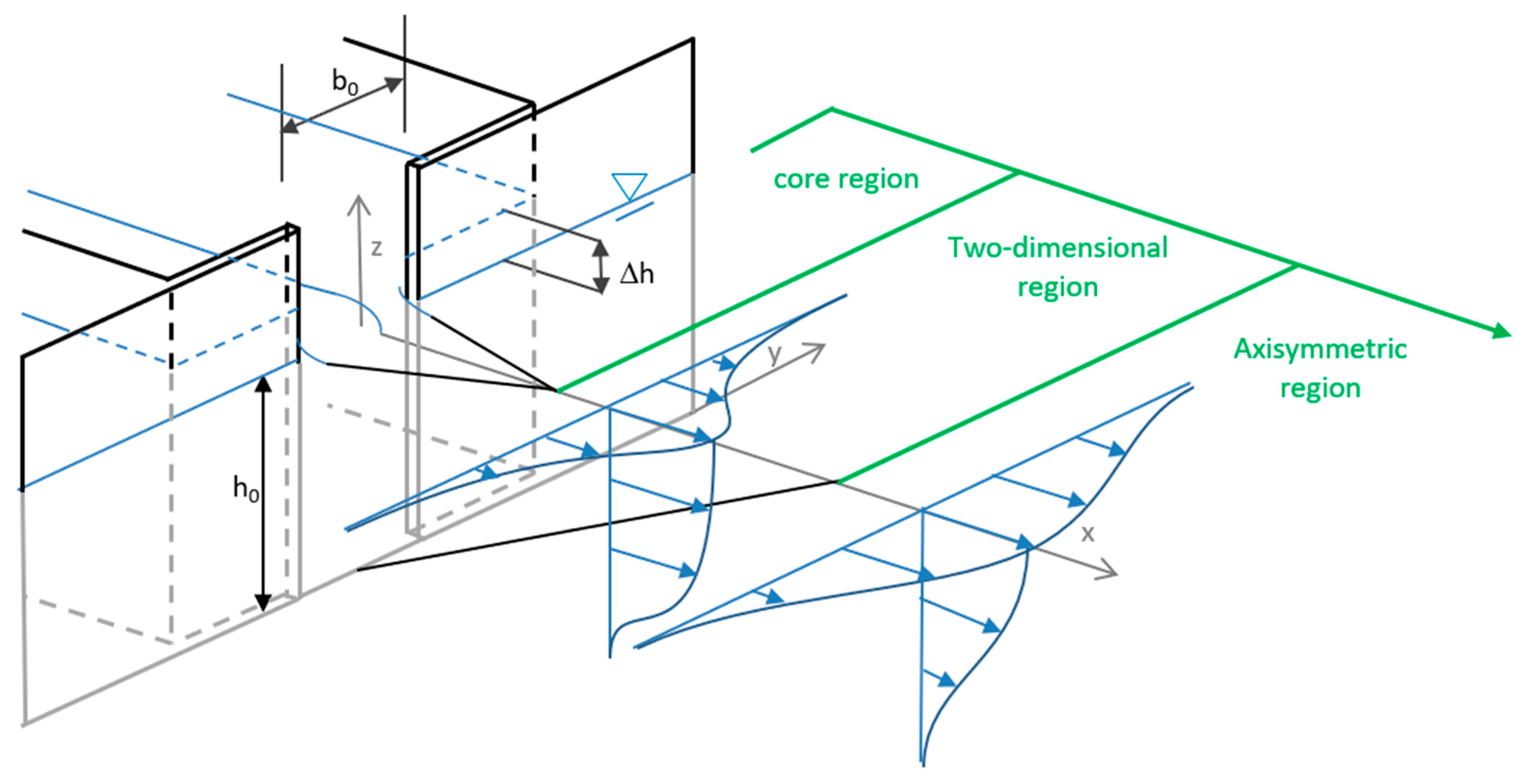
• Orifice geometries of the considered fishways consist of vertical slots [16], which differ from nozzles geometrically and with regard to their hydraulic properties. The local head drop $\mathsf{\Delta }h$ induces shear at the slot margins and forces the jet to submerge at the water surface (Figure 1). In addition, the vena contracta effect causes velocities to increase in and downstream of the slot [11].
• Flow in fishway pools is turbulent [17,18] so that flow approaching the slot is inhomogeneous and highly turbulent, whereas flow approaching a nozzle is approximately homogeneous with a low turbulence level [10,11,12,13]. Furthermore, [19] show that different velocity distribution and turbulence intensities impact jet propagation. These differences may influence the propagation of the jet.
• Tailrace geometry, specifically solid boundaries, may influence jet propagation. Wall effects are common near fishway entrances because of the proximity of a nearby river bank. Wall jets create different propagation characteristics compared to unbounded free jets. For two-dimensional wall jets, propagation length increases because turbulent mixing is suppressed at the walls (e.g., [20]). However, fishway entrances are not located immediately next to a lateral wall but with a small offset distance that is usually in the order of one slot width, so that fish may approach the slot from either side [21]. The Coanda effect forces the jet to attach to the wall and the jet follows the pattern of the wall instead of its initial direction [22]. The distance between the slot and the lateral wall denominated as offset determines the attachment point and consequently influences the propagation characteristics of the jet [23,24,25].

To address (1) to (3), we assessed different fishway boundary conditions in a numerical model. We chose a detached eddy simulation (DES) model to illustrate important hydraulic phenomena present at vertical slots. However, Reynolds-averaged Navier–Stokes (RANS) models are often applied during fishway design processes, as their computational burden is reduced compared with other approaches such as direct numerical simulation (DNS), large eddy simulation (LES), or detached eddy simulation (DES) while still yielding acceptable accuracies. For this reason, we applied both RANS and DES to investigate the accuracy of stand-alone RANS models which are used to simulate the velocity distribution of three-dimensional rectangular surface jets from fishway entrances.

Our review identified significant knowledge gaps that prevent an accurate description of the propagation of attraction flows from prototype fishway entrances. The application of existing equations for jet propagation may not be feasible because of the unique boundary conditions encountered at fishway entrances. Our overall goal was to address these knowledge gaps and to improve the prediction of fishway attraction flow propagation. Specifically, we aimed to: (a) quantify jet propagation with boundary conditions present at fishways; (b) assess our results by comparing them to established analytical jet propagation approaches for three-dimensional rectangular surface jets; and (c) investigate the capability of a RANS model to adequately address the effects of boundary conditions by comparing their output to the output of a DES model.

2. Material and Methods

2.1. Numerical Methods

We used the open source toolbox OpenFOAM 4.1 [26], which provides an integrated framework for numerical calculations in continuum mechanics for three-dimensional computational fluid dynamics (CFD) modelling. We chose the multi-phase solver interFoam for modelling free surface and unsteady flow to discretize the incompressible Navier–Stokes equations. The solver uses the Volume-of-Fluid approach to track the position of the interface between water and air phases [27]. The multi-phase solver using Volume-of-Fluid is applied to account for the head drop at the fishway slot. We applied two different turbulence models: a Reynolds-averaged Navier–Stokes (RANS) model and a detached eddy simulation (DES) model.

RANS models separate the turbulence fluctuations from the mean flow and consider the influence of turbulence on the mean flow by modelling turbulence characteristics. The applied RANS k-ω SST model [28,29] combines the advantages of the k-ω and k-ε model by using k-ω near the wall and k-ε in the free flow region [30]. Only the most relevant equations for the present investigation are given in the following. The k- and ω equations are defined as follows in Equations (1) and (2):

$$\frac{\partial \left(\rho k\right)}{\partial t}+\frac{\partial \left(\rho {\overline{u}}_{j}k\right)}{\partial x_j}={\tilde{P}}_k-\beta \ast \rho k\omega +\frac{\partial }{\partial x_j}\left[\left(\mu +{\sigma }_k{\mu }_t\right)\frac{\partial k}{\partial x_j}\right] \mathrm{and}$$

(1)

$$\frac{\partial \left(\rho \omega \right)}{\partial t}+\frac{\partial \left(\rho {\overline{u}}_j\omega \right)}{\partial x_j}=\alpha \rho S^2-\beta \rho {\omega }^2+\frac{\partial }{\partial x_j}\left[\left(\mu +{\sigma }_{\omega }{\mu }_t\right)\frac{\partial \omega }{\partial x_j}\right]+2\left(1-F_1\right)\rho {\sigma }_{\omega 2}\frac{1}{\omega }\frac{\partial k}{\partial x_i}\frac{\partial \omega }{\partial x_i}.$$

(2)

The turbulent eddy viscosity is defined as follows in Equation (3):

$${\nu }_T=\frac{a_{1}k}{max\left(a_1\omega ,S{F}_2\right)}$$

(3)

$F_1$ is a blending function for switching between the k-ω and k-ε formulation is as follows in Equation (4):

$$F_1=tanh\left\{{\left\{min\left[max\left(\frac{\sqrt{k}}{\beta \ast \omega y},\frac{500\nu }{y^2\omega }\right),\frac{4\rho {\sigma }_{\omega 2}k}{C{D}_{k\omega }{y}^2}\right]\right\}}^4\right\}$$

(4)

with $C{D}_{k\omega }=max\left(2\rho {\sigma }_{\omega 2}\frac{1}{\omega }\nabla k\nabla \omega \right),{10}^{-10}$ and $y$ is the wall distance to the closest wall. $F_2$ is a second blending function (Equation (5)):

$$F_2=tanh\left\{{\left[max\left(\frac{2\sqrt{k}}{\beta \ast \omega y},\frac{500\nu }{y^2\omega }\right)\right]}^2\right\}$$

(5)

To prevent the build-up of turbulence in stagnation regions, a production limiter is included as (Equation (6))

$${\tilde{P}}_k=min\left({\mu }_{t}S,10\beta \ast \rho k\omega \right)$$

(6)

The transient DES model is a combination of LES and time-averaged RANS. Depending on the grid resolution and the distance to the wall, DES changes between the two models, i.e., RANS is used near walls, and the higher accuracy of LES is applied in the other regions. The principle of LES is to reduce computational costs compared to DNS by only solving the large eddies and modelling small scale eddies. In our study, we applied the k-ω SST-DES model [29], which is based on the RANS k-ω SST model. The dissipation term in the k-Equation (1) is modified by $F_{DES}$ for the DES formulation (Equations (7) and (8)):

$$\frac{\partial \left(\rho k\right)}{\partial t}+\frac{\partial \left(\rho {\overline{u}}_{j}k\right)}{\partial x_j}={\tilde{P}}_k-\beta \ast \rho k\omega F_{DES}+\frac{\partial }{\partial x_j}\left[\left(\mu +{\sigma }_k{\mu }_t\right)\frac{\partial k}{\partial x_j}\right]$$

(7)

$$\mathrm{with} F_{DES}=max\left(\frac{L_t}{C_{DES}\mathsf{\Delta }}(1-F_{SSt},1\right) \mathrm{and} F_{SST}=0,F_1,F_2$$

(8)

where Δ is the maximum local grid spacing, $L_t=\frac{\sqrt{k}}{\beta \ast \omega }$ is the turbulent length scale and $C_{DES}=0.61$ is a calibration constant. A weak point of DES is the switch of RANS to LES inside the boundary layer for fine grids. In order to avoid grid-induced separation (GIS) in the wall boundary layer, the blending function $F_{SST}$ is set to $F_2$ [29] so that the RANS simulation is forced in the boundary layer.

2.2. Simulation Setup

The model domain is divided into two main parts, with the exit of the jet forming the reference cross section at $x=0$: the approach flow ($x<0$) and the tailrace ($x>0$) domain. The approach flow $x<0$ acts as a boundary condition for jet propagation (Section 3.1) into the tailrace domain. The symmetry plane is set at $y=0$. The bottom of the approach flow domain (fishway entrance pool or channel bottom) is at $z=0$. In order to avoid spurious boundary effects on the free jet other than the presence of a lateral wall, a broad model domain is chosen for the tailrace with a depth of 11 m ($z=-11$ m), a total length and width of 45 m and 40 m, respectively.

In total, four different jet configurations (Figure 2) are tested, with one channel and three slot geometries.

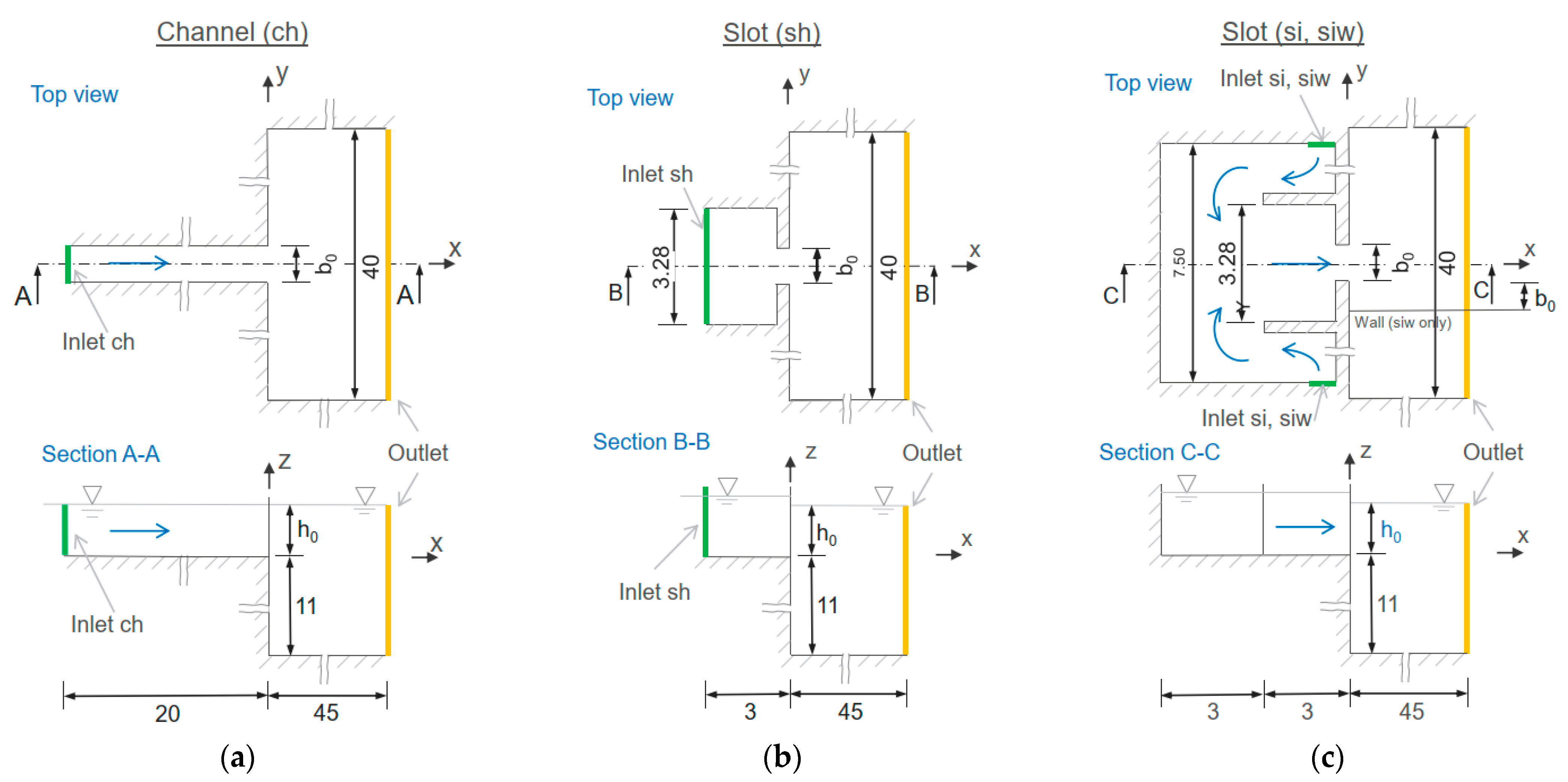
• Channel geometry (ch, Figure 2a) for comparison with previous studies;
• Slot geometry with a homogeneous approach flow (sh, Figure 2b) for investigating the effect of a slot;
• Slot geometry with an inhomogeneous approach flow (si, Figure 2c wall not included in the model domain) for identifying the effect of approach flow in combination with a slot;
• Slot geometry with an inhomogeneous approach flow and lateral wall in the tailrace (siw, Figure 2c wall included in the model domain) for determination of the effect of river bank in the tailwater.

We selected the configurations to represent a range of possible upstream flow characteristics and two different tailrace conditions. The channel configuration (ch) with slip boundary conditions is comparable to a nozzle configuration and consists of a channel profile entering the tailrace at $x=0$ (Figure 2a). The three slot configurations (sh, si, siw) consist of a basin with a vertical slot at $x=0$ m, but with different upstream and tailrace geometries. For the sh configuration, the approach flow to the slot is homogeneous to provide the least possible turbulence intensity and velocity fluctuations at the slot orifice at $x=0$ (Figure 2b). At the inlet, a uniform velocity distribution is assigned to avoid an increase in turbulence intensity, i.e., no significant shear zones or wall effects exist. For the si configuration, we followed [31,32], who showed that two opposed jets result in a high turbulent intensity. The two inlets are located at position inlet si in Figure 2c. Thus, the water is forced to flow around two walls, resulting in an increase of turbulence intensity to achieve an inhomogeneous, highly turbulent approach flow at $x=0$. Both configurations sh and si deviate from the real situation in a fishway entrance pool, where different flow situations exist due to a large variety of pool designs [18,33,34]. The chosen configurations represent two extrema: an ideally homogeneous approach flow with a low turbulence intensity (sh) and an artificial, highly turbulent situation with an inhomogeneous approach flow, which is unfavorable for a fishway entrance pool (si). The siw configuration uses the si layout but adds a lateral wall in the tailrace to represent the river bank usually located near the slot of fishway entrances (see Figure 2c). We set the distance of the wall to the slot to be one slot width $b_0$, which is often applied in practice and is a compromise between the sufficient width for the fish access on either side of the slot, but narrow enough to allow the jet to attach to the wall in order to propagate further downstream.

In sh, si, and siw, beveled slots are applied, which are preferred to sharp-edged slots for constructability and to reduce fish injuries during passage [16]. All configurations were modelled with RANS and DES (summarized in

Table 1. Properties of simulated cases.

Configuration	Case Name	Tailrace Condition	Orifice Geometry	Turbulence Model	Approach Flow
ch	ch-rans	Surface free jet	channel	RANS	homogeneous
ch	ch-des	Surface free jet	channel	DES	homogeneous
sh	sh-rans	Surface free jet	slot	RANS	homogeneous
sh	sh-des	Surface free jet	slot	DES	homogeneous
si	si-rans	Surface free jet	slot	RANS	inhomogeneous
si	si-des	Surface free jet	slot	DES	inhomogeneous
siw	siw-rans	Surface wall jet	slot	RANS	inhomogeneous
siw	siw-des	Surface wall jet	slot	DES	inhomogeneous

).

The basic grid resolution is set to 0.4 m, which is too coarse to model jet evolution, but is adequate for the regions that the jet does not reach. Consequently, cell resolution in the channel/entrance pool and regions in the tailrace reached by the jet are refined to 0.05 m for 0 < x ≤ 16 m and −4 ≤ y ≤ 4 m for the RANS simulations. The refinement region is enlarged up to x=30 m and to −8 ≤ y ≤ 8 m for the DES simulations to achieve accurate results in the far field with the DES model. In the vertical direction, the tailrace is refined for −2 ≤ z ≤ 1.5 m to adequately reproduce the water surface. The cell size in the slot and the channel profile respectively does not exceed 0.0125 m for a width of 0.45 m, which equals 36 cells. The region close to the water surface is additionally refined to 0.025 m in vertical direction. The mesh discretization within the slot was determined by sensitivity studies where only the chosen grid size was fine enough to reproduce the velocity distribution in the slot. The total number of grid cells varies and is approximately between 7 × 10⁶ and 8 × 10⁶ for all configurations modelled with RANS. The grids of the DES simulations have about 16 × 10⁶ cells.

We omitted sensitivity analyses of the overall grid size in the jet evolution region because the results of the ch configuration simulated with RANS and DES fit well to comparable data about decay rate and lateral spreading from literature [7,8,14].

2.3. Boundary Conditions

The boundary and initial conditions are derived from typical values for fishway entrance designs usually applied to German rivers. The spatial average velocity (bulk-mean) in the orifice cross section for the channel and the slot is set constant to $u_0=1.37$ m/s, which yields a discharge of $Q=0.74$ m³/s and a head loss at the slot of about 0.12 m. In all simulations, the channel and slot width is $b_0=0.45$ m and the water depth is set to $h_0=1.2$ m, which is a common biological requirement for flow depth in fishways of German waterways. The Reynolds number, based on orifice width $b_0$, is 6.17 × 10⁵. The Froude number in the orifice is 0.40 and, therefore, flow is sub-critical.

The RANS simulations are initialized to a water level of 1.2 m. All other variables except at the fluid boundaries are initialized at zero. In order to optimize simulation time, the DES simulations are initialized with the mapped values of the results of the RANS simulations. The boundary conditions for RANS and DES are set as:

• inflow boundary of ch and sh: inlet velocity boundary with a flowrate of 0.74 m³/s; turbulence intensity = 0;
• inflow boundaries for si and siw: two inlet velocity boundaries with a flowrate of 0.37 m³/s each; turbulence intensity = 0;
• outflow boundary: pressure outlet boundary with a fixed water surface of 1.2 m and a water density of 1000 kg/m³;
• wall boundaries except the slot geometry and the walls of the entrance pool: slip boundary conditions without friction for velocity; and
• wall boundary in the entrance pool and at the slot: fixed value of velocity = 0 m/s and a wall function with wall roughness $k_S=0.005$ m.

The run time for the RANS simulations is 480 s and 660 s for DES. The first 300 s ensures a state independent from initial conditions. The subsequent 180 s (RANS) and 360 s (DES), resp., are averaged to obtain best possible stationary results.

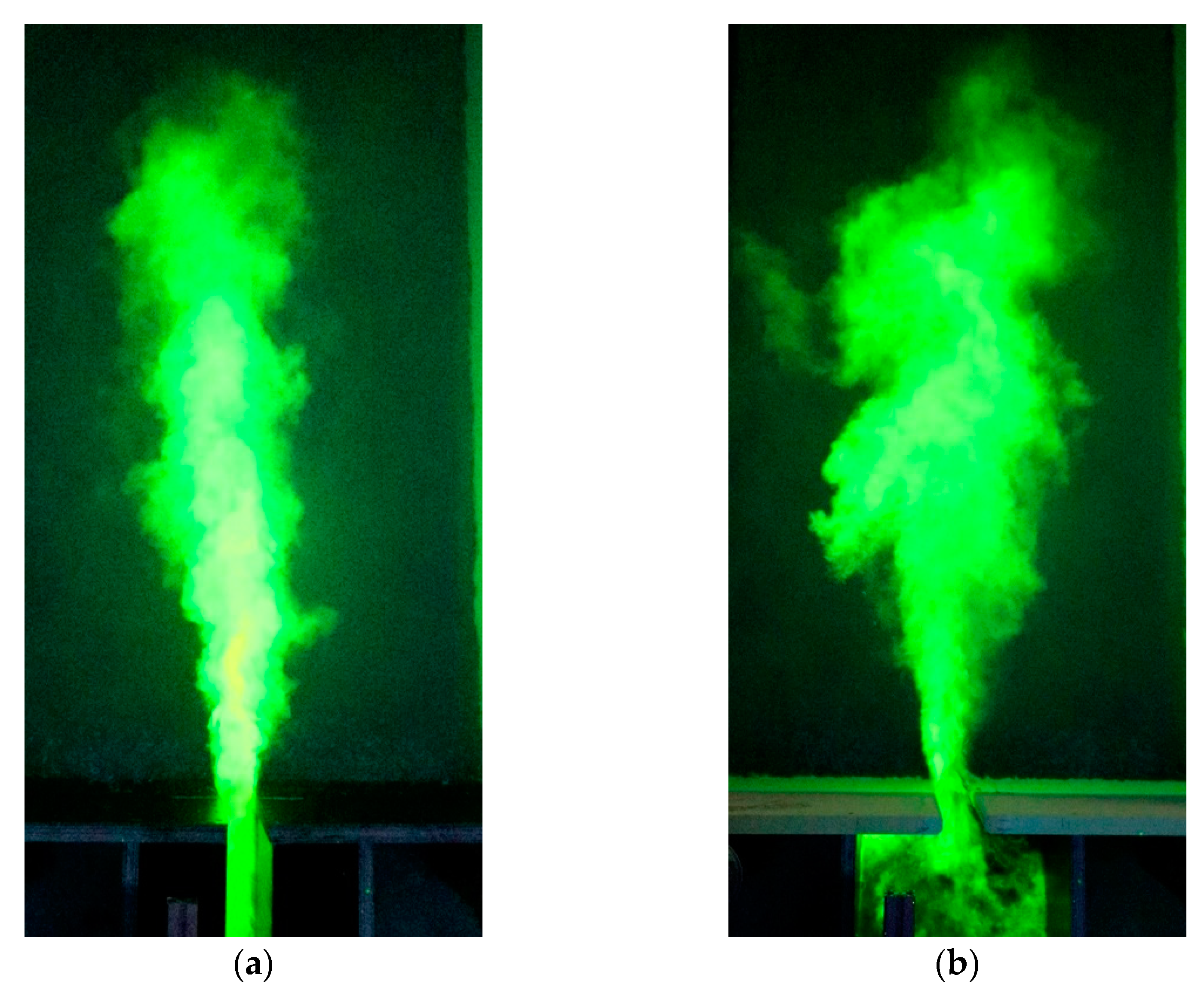
2.4. Additional Physical Scale Model Investigations

The propagation of the channel jet (ch) and the slot jet with inhomogeneous approach flow (si) were additionally investigated in an experimental flume at BAW. The geometry of the inlet apparatus is the same as for the numerical model with a geometric length and height scale of 1:7.5. The tailrace is 2 m long, 1.2 m wide and 0.4 m deep. Water is added from a constant-head tank through a tubing system. The discharge is regulated with a slide valve and an inducted magnetic discharge sensor. The tailrace water level is regulated with a tilting weir. The flow is visualized using fluorescent dye illuminated with a black light. Digital images from the top (1.5 m height) are recorded at a rate of 25 frames per second [35].

3. Results

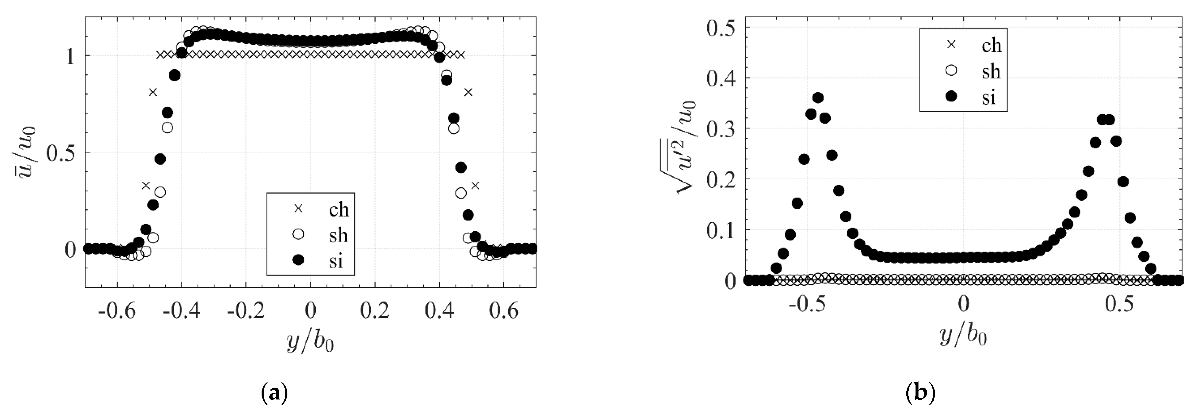
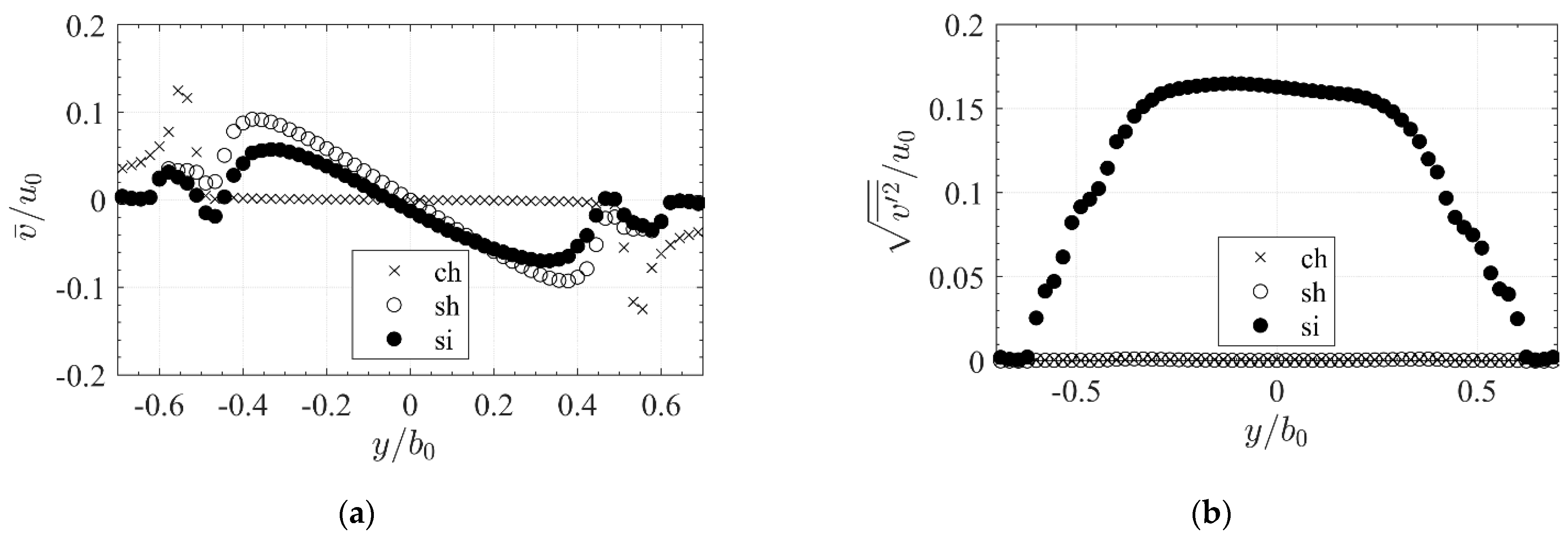
3.1. Approach Flow Velocity Distributions

To point out the differences in approach flow of the ch, sh and si configurations we evaluated the velocity distribution and turbulence intensity at the orifice exit section ($x=0$) and the cross section of x = −3 (inlet sh) for the DES simulations (Figure 3, Figure 4 and Figure 5). Both RANS and DES, yielded similar results for the mean velocity distribution.

The distribution of normalized time-averaged velocities $\overline{u}/u_0$ in the streamwise direction of the channel configuration ch-des at the orifice exit section ($x=0$) are homogeneous at $\overline{u}/u_0=1,$ whereas the slot configurations sh-des and si-des show a slight increase of velocities up to 1.1 $u_0$ at the edges (Figure 3a). The velocity peaks of sh are slightly more pronounced compared to si. All slot configurations produce recirculating flow close to the edges of the slot. The configurations ch-des and sh-des show a very low level of turbulence (Figure 3b), whereas the turbulence intensities of si-des are distinctly higher (up to $\sqrt{\overline{{u\prime }^2}}/u_0=0.3$).

The normalized time-averaged lateral velocities $\overline{v}/u_0$ in the orifice exit of ch-des are mostly homogenous whereas $\overline{v}/u_0$ of sh-des and si-des show the constriction effect of the slot towards the centerline (Figure 4a). The peaks of the sh-des jet ($\overline{v}/u_0=0.09)$ are higher than those of the si-des jet ($\overline{v}/u_0=0.06$), but the fluctuations of si-des are more distinct and even larger than the mean velocities (up to $\sqrt{\overline{{v\prime }^2}}/u_0=0.17$, Figure 4b). For all configurations, fluid is entrained from outside of the jet (Figure 4a).

sh-des and si-des have different velocity distributions and turbulence intensities in the cross section of $x=-3$ (Figure 5). For the sh jet, a constant velocity distribution and zero turbulence intensity are applied at inlet sh ($x=-3$). The si jet shows a normalized velocity peak at $y=0$ m of $\overline{u}/u_0=0.35$ and a back flow of about $\overline{u}/u_0=-0.1$ close to the walls. The normalized turbulence intensity $\sqrt{\overline{{u\prime }^2}}/u_0$ at these positions is up to 0.12. The inlet conditions of the siw case are equal to the si case.

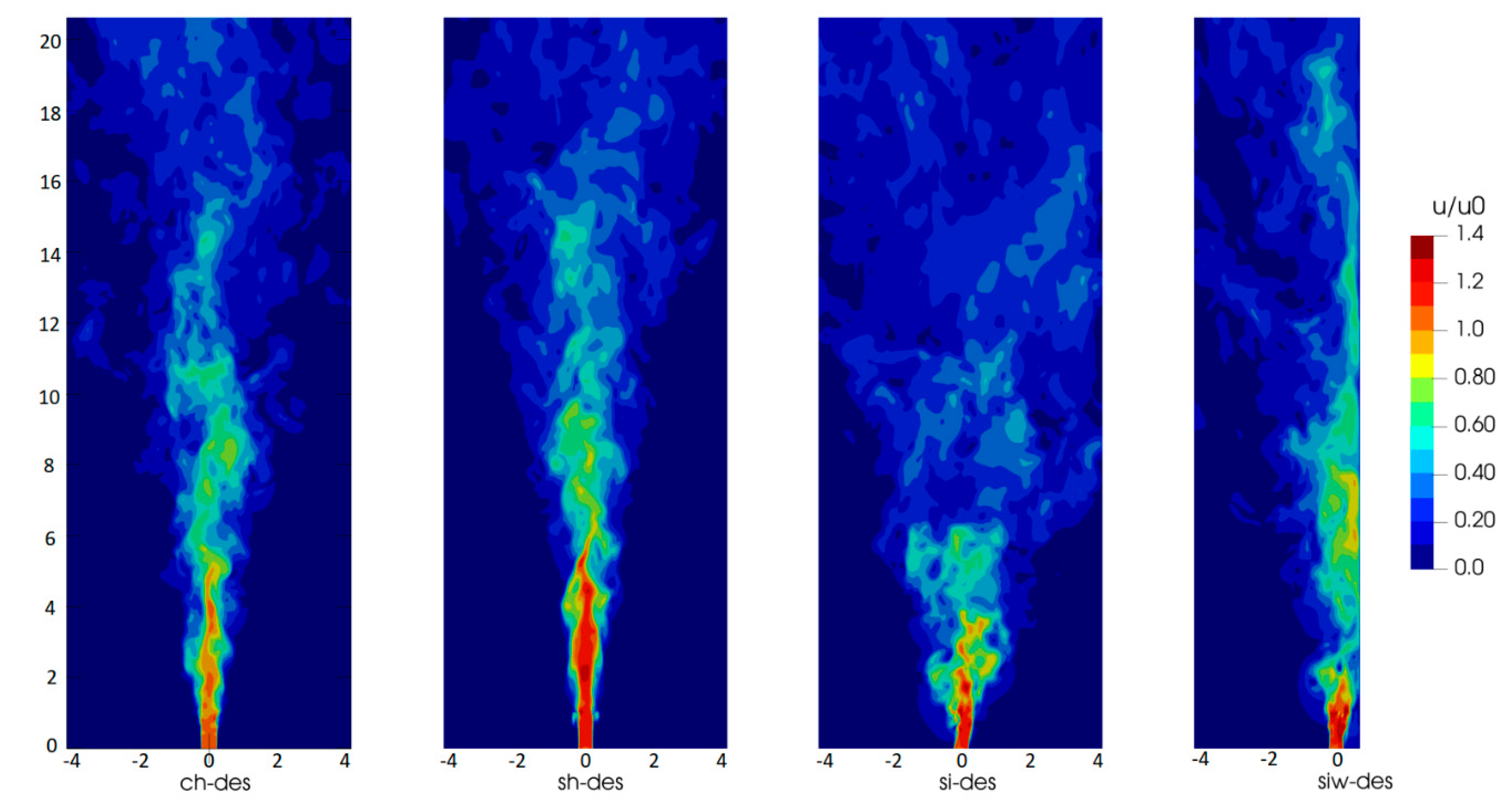
3.2. Qualitative Assessment of the Jet Velocity Fields

We used a screen capture of the DES model output to qualitatively compare jet propagation of the different configurations (Figure 6). The ch jet propagates downstream near the centerline with low lateral spreading. It is characterized by a pronounced core zone. The sh jet also propagates around the centerline but the velocities in the core zone are increased and reach further into the tailrace compared to ch. Velocities in the far field are similar. In contrast, the propagation of si jet is characterized by a more pronounced lateral spreading and a shorter core zone. In the far field, a distinct jet is no longer visible. Furthermore, the wall jet (siw) has a short core zone and starts to attach to the wall at x = 2 m. The jet concentrates near the wall and shows less lateral spreading than si.

We used a frame grab of the video of tracer concentration in the scale model to qualitatively describe jet propagation for the ch and si configurations (Figure 7). The ch jet concentrates along the centerline whereas the si jet spreads more in a lateral direction. Note that the DES model output and scale model results show good qualitative accordance for the ch and si configurations.

3.3. Influence of Slot and Approach Flow on Free Jet Propagation

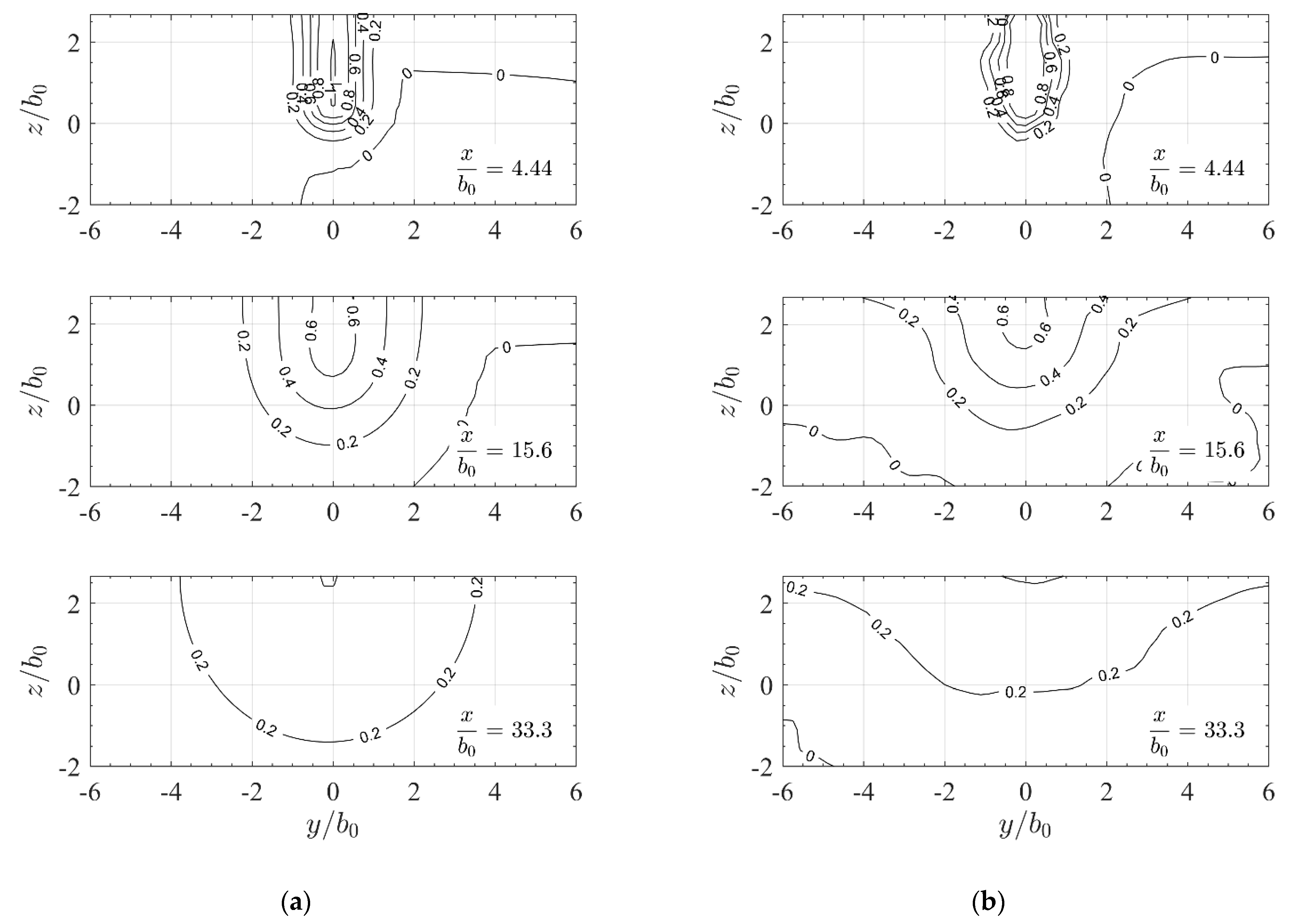
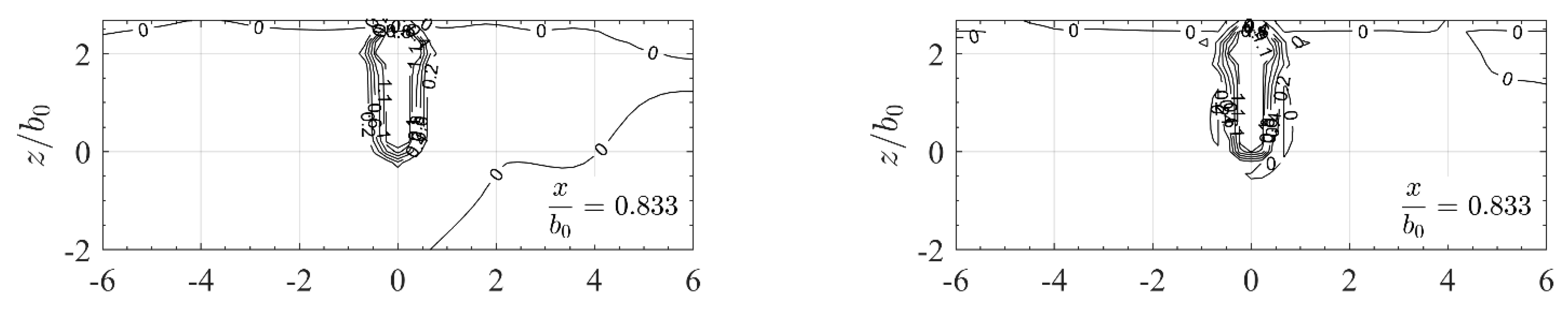
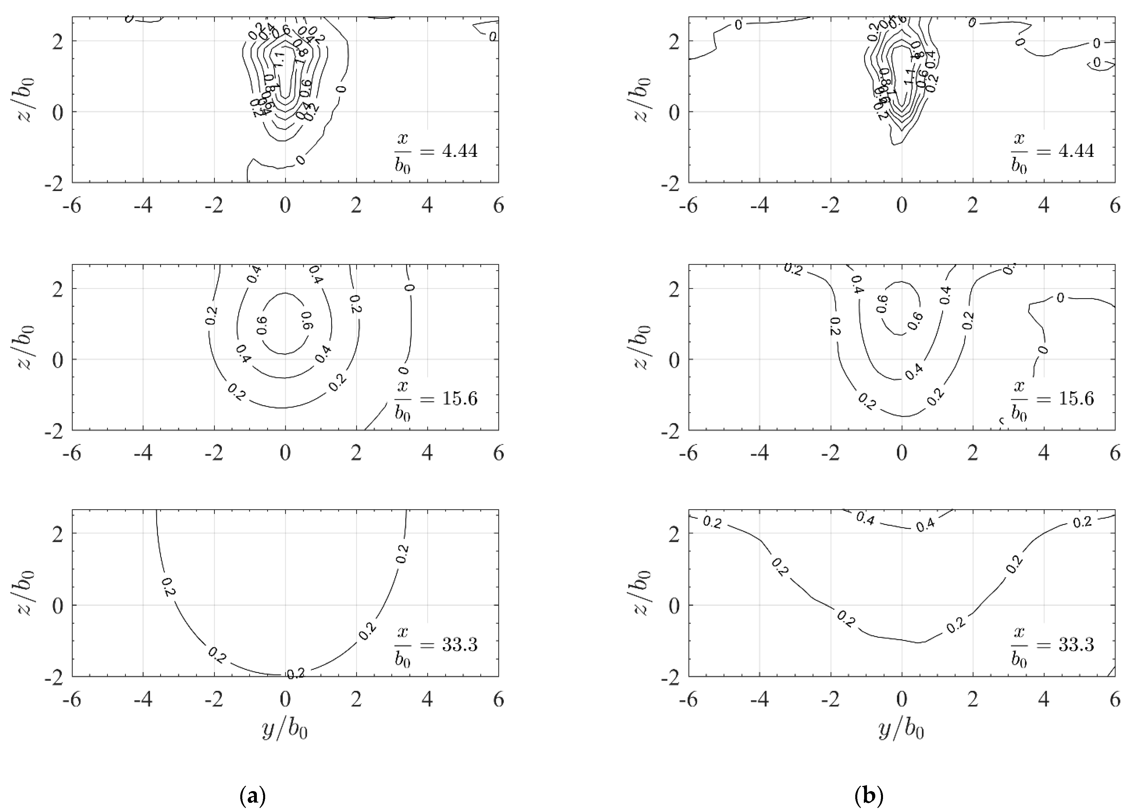
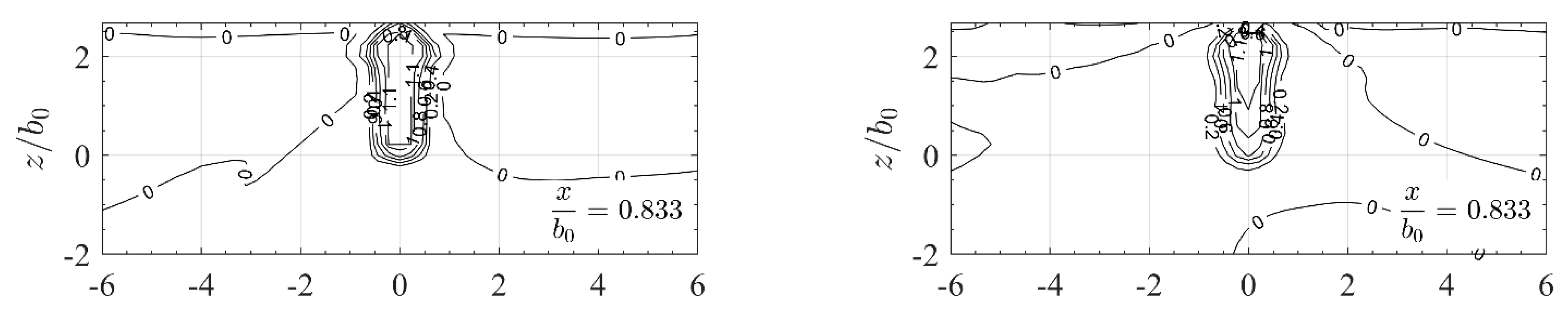
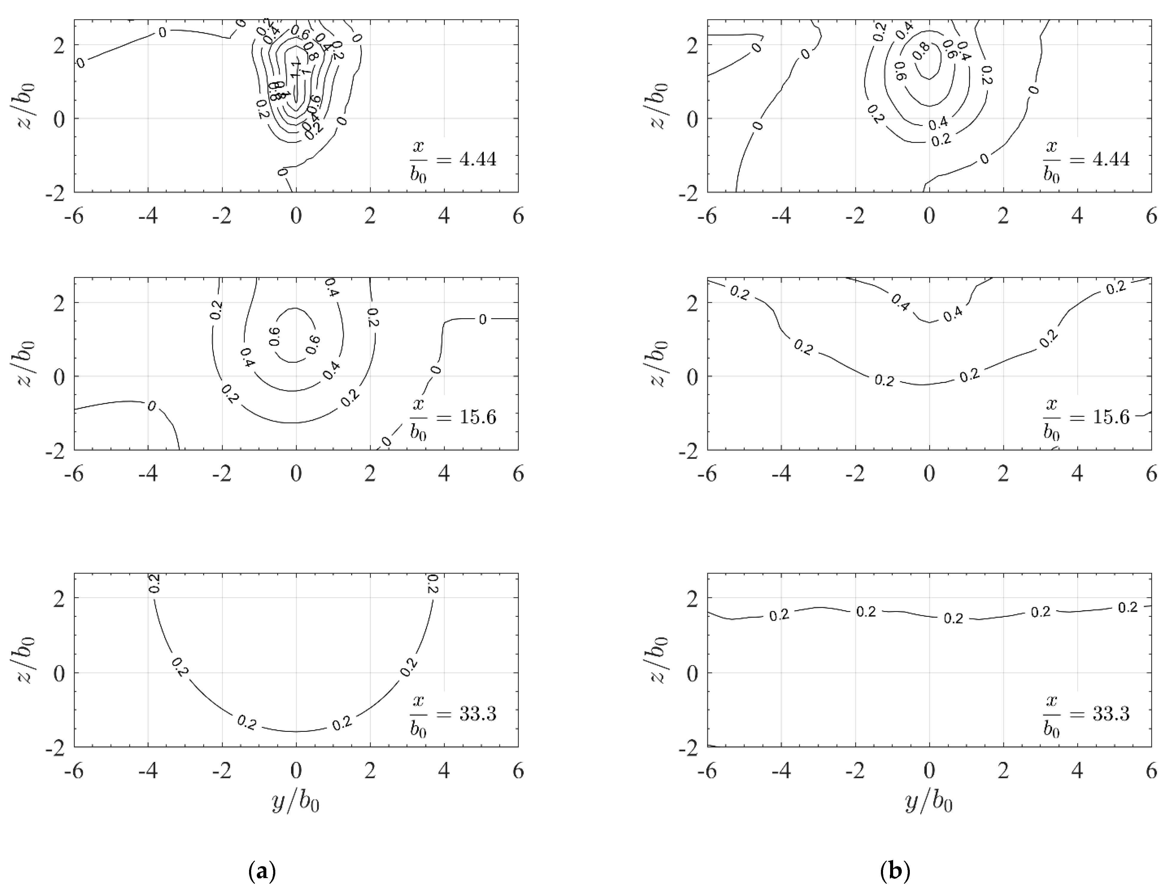
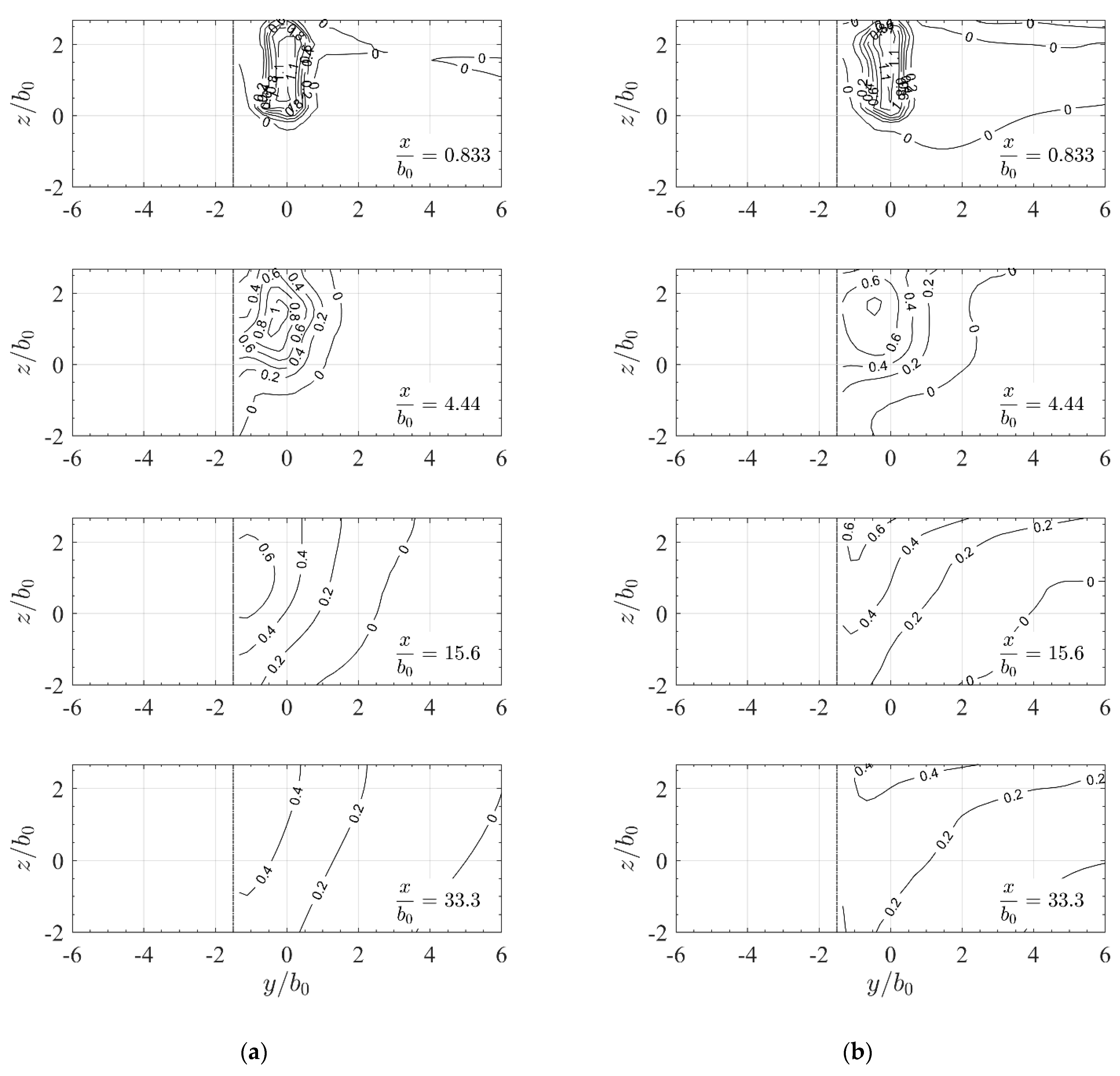
3.3.1. Velocity Fields

In order to assess spatial jet propagation, distributions of time-averaged streamwise velocity components $\overline{u}$ in vertical yz-planes were evaluated at various distances $x>0$ representing different jet regions for RANS and DES (Figures 8–10). In all subfigures, the velocity is normalized with mean velocity $u_0=Q_0/(b_0{h}_0)$. Distances $x$ are normalized with channel/slot width $b_0$.

The velocity fields output by the ch-rans and ch-des models are similar and show the typical characteristics of rectangular jets (Figure 8). The three typical jet regions can be identified: (1) the primary core region with the core velocity of $\overline{u}/u_0$ and the rectangular shape imposed by the orifice is present directly downstream of the exit ($x/b_0=0.833$ and $x/b_0=4.44$); (2) followed by the two-dimensional region ($x/b_0=15.6$); and (3) the axisymmetric region at $x/b_0=33.3$. The ch-des jet shows a more distinct lateral spreading at the surface in the axisymmetric region than the ch-rans jet.

The RANS and DES model results for the sh jet show initial similarities near the slot and slightly deviate progressively with the distance from the slot (Figure 9). Initially, at $x/b_0=0.833,$ the jet has the rectangular shape imposed by the orifice and propagates at the surface. The core region with core velocity of $u/u_0=1$ can be identified at $x/b_0=0.833$ and 4.44 where the jet is submerged. The submergence effect results from the vertical velocity component as induced by the water level difference at the slot. At $x/b_0=15.6,$ the two-dimensional propagation is less pronounced but can still be identified and at $x/b_0=33.3$ an axisymmetric region can be discerned. The general shapes of the jet propagation predicted by the DES and RANS models are similar, but the DES simulations exhibit a slightly more intensive lateral spreading.

The velocity profiles of si-rans show similar velocity distributions as the sh jet (Figure 10a). The core region extends up to $x/b_0=4.44$ and the submergence effect is apparent at $x/b_0=4.44$ and 15.6. The two-dimensional ($x/b_0=15.6$) and axisymmetric regions ($x/b_0=33.3$) can be identified. Close to the orifice at $x/b_0=0.833,$ si-des is similar to si-rans (Figure 10b). However, further downstream, the DES simulations show a different propagation compared to all the other simulations. The core velocity is already reduced at $x/b_0=4.44$, and thus the transition to the two-dimensional region occurs earlier. In the far field at $x/b_0=33.3,$ no distinct axisymmetric zone develops. The lateral propagation of the transient si-des jet is distinctly larger than that of the si-rans jet.

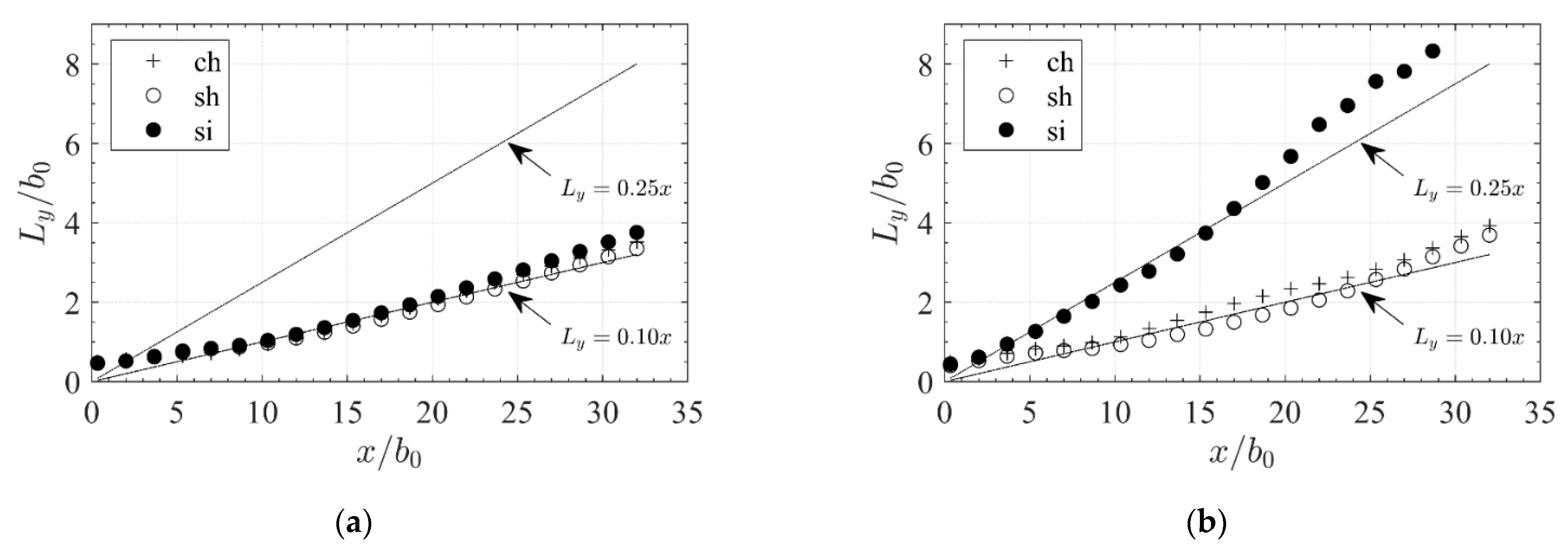
3.3.2. Jet Half-Width Growth

We used the jet half-width $L_y$ at $z=0.5 h_0$ as a metric to describe the lateral spreading of the propagation jets as simulated by the RANS and DES models (Figure 11). Here, $L_y$ is the distance in the y-direction from the jet center, characterized by the local maximum velocity, to the location where the time-averaged velocity is half the local maximum. We define $L_y$ as the mean value of the left- and right-side half-widths and calculate it from the corresponding lateral velocity profiles. The growth of the half-widths is approximated by linear expressions $L_y/x$. The lateral growth rates of the ch and sh jet are determined to $L_y/x=0.10$ for both RANS and DES models. This value is comparable to the growth rates for plane and rectangular surface jets ([14,15,22],

Table 2. Lateral growth rates in literature.

Paper	Jet Type	${\mathit{L}}_{\mathit{y}}/\mathit{x}$
Miozzi et al. [22]	Plane surface jet	0.10
Kashi [15]	Rectangular surface jet	0.12
Rajaratnam and Humphries [14]	Circular or rectangular surface jet	0.09
Present study	Rectangular surface channel jet (ch)	0.10
Present study	Rectangular surface slot jet (sh)	0.10
Present study	Rectangular surface slot jet (si)	0.25

). The lateral growth rates are the same for all configurations (ch, sh, si) using the RANS model (Figure 11a). However, the si slot configuration differs substantially using the DES model (Figure 11b). $L_y/x$ of si-des can be approximated to 0.25, about 2.5 times the growth rate of the RANS simulations. This value is consistent with the differences in spatial jet propagation, where a more pronounced lateral spreading of the jet was observed (Section 3.3.1).

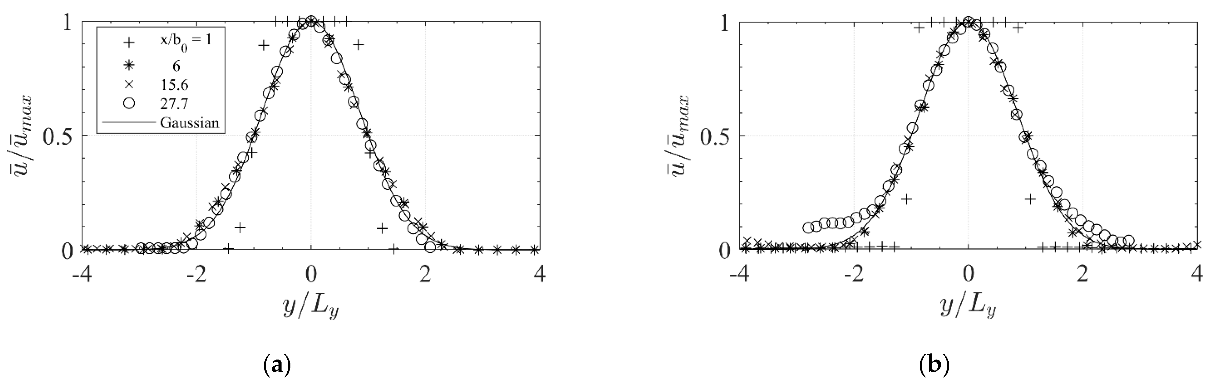
3.3.3. Self-Similarity

The lateral distributions of $\overline{u}$ in the height $z=0.5 h_0$ normalized by the local velocity maximum ${\overline{u}}_{max}$ on the centerline at the respective $x$ was used to assess self-similarity in the propagation of the jet [36] (Figure 12). Locations $y$ are normalized by $L_y$. The symbols represent the distributions at four distances $x/b_0$ from the orifice. For comparison, the normalized standard Gaussian function is plotted. The potential core zone with the non-Gaussian distribution is present for all simulations at $x/b_0=1$. Outside the potential core zone, the profiles for all cases approach the Gaussian distribution, indicating the self-similar development of the jets. The transient DES simulations slightly deviate from the Gaussian distribution in the far field, suggesting that the temporal averaging time of 360 s is still not sufficient to exactly represent the si jet in the far-field. However, in general, self-similarity is reached for all jets independently of the simulated configuration.

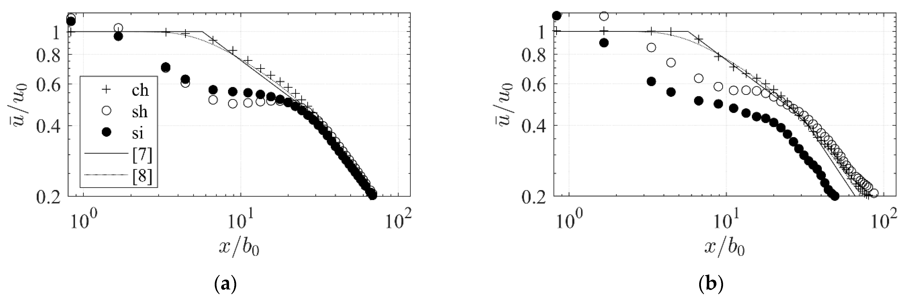
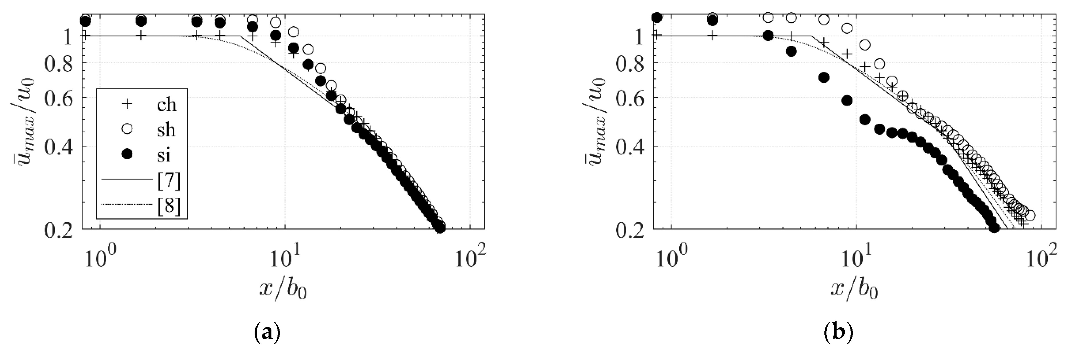
3.3.4. Velocity Decay

We compared downstream evolution of streamwise mean velocities at the water surface to analytical approaches [7,8] (Figure 13). The evaluation along the water surface centerline is used since the maximum velocity is located at the water surface and along the centerline for surface jets from nozzle orifices and in theoretical models. All velocities are normalized by the bulk-mean exit velocity $u_0$. The ch jet shows good agreement for the entire range of velocities at the water surface when compared to theoretical decay for both simulation methods (Figure 13a,b). Transition locations between the characteristic zones (from core zone to two-dimensional region at $x/b_0\approx 6$ and from the two-dimensional region to the axisymmetric region at $x/b_0\approx 30$) are predicted correctly. In contrast, both slot jets show higher velocities close to the exit caused by the vena contracta effect at the slots. Downstream of the exit, $u/u_0$ substantially decreases until $x/b_0=7$ because of the water level drop at the slot and the corresponding jet submersion. The flow reattaches the surface at approximately $x/b_0=20$. Thereafter, the jet develops similar to axisymmetric jets. In the near field, the decay is strongly influenced by these effects for both types of approach flow for the slot jets (sh and si). However, both effects are not appreciable in the far field for sh jet where its velocity decay follows the same trend as the ch jet, which is in accordance with [11]. In the far field, there is no difference in surface velocities among ch, sh, and si-rans configurations. However, streamwise surface velocities in the far field of si-des are reduced by 30%. The reduction is consistent with the higher lateral growth rates of the jet observed in Section 3.3.3. It should be noted that the velocities downstream $x/b_0=66$ are subject to inaccuracies because of grid resolution effects.

The analysis of centerline velocities at the water surface cannot be exhaustive for slot jets due to the submergence of the jet. Additionally, maximum streamwise velocities independent of their location in the yz-plane were determined for every time step, temporally averaged and normalized by $u_0$ (Figure 14). The velocity decay of the ch jet is similarly compared to the centerline velocity at the surface for both simulation methods. Only velocities in the two-dimensional region are slightly higher for ch-rans compared to the velocities at the water surface. In contrast, there is a large difference between the surface velocity and the maximum velocity for all slot jets in the two-dimensional region. This confirms that the maximum velocities of the slot jets are below the water surface. The core zone of sh-des is significantly larger than the core zone of si and ch. For the si-des jet the maximum velocities substantially decrease in the two-dimensional zone and are reduced by about 25% compared to the ch jet in the far field.

The half-length $L_x$ defined as the longitudinal distance from the orifice exit, where $\overline{u}/u_0=0.5$, is evaluated as a further measure to compare jet propagation. For homogeneous approach flows, ch and sh, $L_x/b_0=24$ correspond well to the half-length derived from analytical expressions [7,8] independent of the simulation methods. Half-length for the slot with an inhomogeneous approach flow si is about 2.3 times shorter ($L_x/b_0=11$) as computed with DES while results computed from si-rans are substantially longer ($L_x/b_0=22$).

3.4. Influence of a Lateral Wall on Jet Propagation

We used the distributions of time-averaged streamwise velocity component $\overline{u}$ of the jet with an inhomogeneous approach flow and lateral wall in the tailrace (siw) of RANS and DES simulations in order to assess spatial jet propagation in the presence of a lateral wall (Figure 15). The core zone for both models can be identified at $x/b_0=0.833$ and the submergence effect is visible at $x/b_0=0.833$ and $x/b_0=4.44$. The presence of the wall triggers the typical behavior of an offset jet [25]. The jet starts to deviate from the centerline ($y=0$) at $x/b_0=4.44$ and attaches to the wall at $x/b_0=15.6$ due to the Coanda effect [22]. The transient simulated siw-des jet ascends to the surface earlier ($x/b_0=15.6$) than the time-averaged siw-rans jet ($x/b_0=33.3$).

The development of wall jets was compared to that of free jets by examining the evolution of jet half-width $L_y/b_0$ with the downstream location (Figure 16a). The results of siw-rans suggest a relatively constant growth rate for half-width, which is lower than that of a free jet simulated with RANS (si-rans) where growth rates of 0.1 are determined. In contrast, the siw-des results show a more distinct behavior where development of the half-width can be divided into two regions in which the first is associated with the free flow region and the second with the influence of the lateral wall. In the first region close to the orifice exit, the growth rate of the half-width is approximately 0.25, which is identical to that of the free slot jet (si-des). Beginning at $x/b_0=6,$ the growth rate substantially decreases until the half-width transitions to a local minimum at $x/b_0=12$ because of the attachment of the jet to the wall. Further downstream, the half-width increases at a constant growth rate of 0.65, which is identical to the experimental results of plane jets with the same wall distance to slot width ratio reported in [24].

We further compared the decay of the maximum velocities of the wall slot jets (siw-rans and siw-des) to the results for the free slot jet (si-rans and si-des) to assess the influence of a lateral wall on the downstream evolution (Figure 16b) of RANS and DES modeling. The results obtained by both simulation methods indicate that a slot jet with lateral wall produces velocities that are higher than those of the free jet. The half-lengths $L_x/b_0$ of the siw-rans jet and siw-des jet are 35 and 29, respectively. Thus, $L_x/b_0$ $of$ siw-rans is 1.6 times larger than the one of si-rans and $L_x/b_0$of siw-des 2.6 larger than the one of si-des. Compared to the free ch and sh jet, the half-length of siw-des is 1.16 larger. Notably, results of both simulation methods differ less for the wall jet than for the free jet. Between $x/b_0=20$ and 40 results of the siw-rans and siw-des are comparable (10–15% deviation), whereas in the far field the deviation increases (20–26% deviation).

4. Discussion

The results of DES modelling show systematic differences in downstream propagation of slot jets for homogeneous and inhomogeneous approach flows. Slot jets with homogeneous approach flows are consistent with [7,8], while slot jets with inhomogeneous approach flows show an increased lateral growth rate of time-averaged streamwise velocities and a reduced downstream propagation in the far-field. The results suggest that the differences in propagation arise from an interaction between the slot and its approach flow conditions. Under inhomogeneous conditions, the velocity distribution at the orifice exit section shows that both streamwise and lateral velocities exhibit strong temporal fluctuations. These fluctuations are associated with oscillations of the jet apparent in the transient numerical DES simulations and in the experimental investigations. In a time-averaged representation, these oscillations are shown in a larger lateral expansion and decreased streamwise velocities of the jet. The instantaneous characteristic under inhomogeneous approach conditions are not significantly broader than under homogeneous approach conditions, but lateral jet oscillation results in an increased lateral manifestation of time-averaged velocities. This assumption is supported by the finding that there is a large difference between centerline velocities and maximum velocities (Section 3.3.4) because the local velocity maximum shifts its position on either side of the centerline in every instantaneous moment and is rarely on the centerline itself. Similar effects of oscillating jets are observed in fishway pools [37] and jets issued from fluidic oscillators (e.g., [38]).

Results of a slot jet propagation with a lateral wall downstream of the slot suggest that oscillations are reduced due to the Coanda effect [22]. The jet shows the above-described behavior with strong oscillations and increased lateral growth rate before it begins to incline towards the wall. After a transition phase the jet attaches to the wall and shows typical lateral growth rates that are consistent with findings of pure wall jets [24]. We assume that this characteristic is largely an effect of the offset distance. At zero offset, oscillation will hardly occur while for large offsets oscillations may possibly overrun the Coanda wall effect and the attachment might be impeded. A comprehensive study of offset distance might be a future research direction.

A variety of entrance pool designs may be encountered during the planning of new fishways or the modification of existing fishways, each of which goes along with its own specific approach flow to the entrance slot. Parameters that may affect the turbulent conditions are among others: geometry of entrance pool, deviation of layout (straight pool or turning pool), distance to upstream slot, slot velocity, and the way auxiliary discharge is added. In the absence of standard design rules for entrance pools, we considered two extreme scenarios: a homogeneous approach flow with low turbulence and an inhomogeneous approach flow with high turbulence. The inhomogeneous and highly turbulent conditions are generated by the collision of two opposing flows to produce large scale eddies larger than in real fishway pools. We assume that the effect of approach flow on jet propagation is therefore less pronounced in real fishways and, as a consequence, the use of the results obtained may be considered as a conservative approach for assessing the attraction jet propagation.

Moreover, the lateral distance from the entrance slot to the river bank or lateral wall is subject to site-specific constraints. Our results are obtained for lateral wall distance of a slot that is equal to one slot width, representing a value which is in a typical range for fishways adjacent to river banks. For smaller distances, an application of our results is conservative since a faster wall attachment results in increased propagation with higher velocities. When offset distances between the slot and the wall increase, downstream propagation of the jet will further reduce until the wall effect becomes negligible and converges towards the jet without a lateral wall.

We additionally applied a RANS model because they are the tools of choice for engineering design of fishways, even though the more complex DES model includes a more complete description of the physics of water flow. The application of DES models may be the exception because its complexity leads to increased difficulty of use and high computational costs. The results show that the propagation of jets with homogeneous approach flows with low turbulence velocity distributions are reproduced reasonably well by RANS models and only differ slightly from DES model results. Small differences may arise from the isotropic turbulence model in RANS, which cannot adequately reproduce surface currents [39]. This observation holds for both channel and slot orifice shapes. In contrast, highly turbulent approach flows of vertical slots cause flow velocities to be significantly overestimated by a RANS model. For RANS models, turbulence is transported as scalars (here k and ω) and it is not possible to resolve the turbulent quantities in the time-averaged mean flow. Consequently, the physical processes are not resolved as evidenced by the fact that the RANS simulations for both approach flows of the slot are similar. To apply other two-equation RANS models than the k-ω SST model we used would not enhance RANS because the turbulent quantities would still not be resolved. Reynolds Stress Models can be used to improve the simulation of surface currents due to the anisotropy of turbulence but the oscillations are also not represented by these models.

RANS model predictions improve progressively as turbulent fluctuations play a reduced role in jet propagation. This is the case for the investigated jet when the lateral wall is in a short distance from the slot. RANS models can better resolve the flow after having been attached to a lateral wall. The remaining differences arise because we simulated an offset jet and therefore the influence of the wall is not present until the flow attaches to the wall. Until this occurs, fluctuating forces dominate which are not resolved by RANS. For pure wall jets with no offset to the wall, RANS modeling showed good agreement to experimental data for velocity distributions [40]. In summary, RANS simulations may be appropriate as long as turbulent fluctuations are not the predominant driver of the flow. Modelers who use RANS for inhomogeneous, highly turbulent approach flows should be aware that the length of jet propagation may be overestimated.

Analytical methods for nozzle jets do not represent the submergence effect at slots but may be used to predict the evolution of centerline velocities in the axisymmetric region for slot jets with a homogeneous approach flow. However, the equations with the given shape parameters do not represent jet propagation of slots with an inhomogeneous approach flow, as shape parameters are calibrated to the boundary conditions given by nozzles that differ in orifice geometry and approach flow.

Summarizing, the results show that the combination of a vertical slot with an inhomogeneous and turbulent approach flow typical for fishway entrances reduces the length of attraction flow compared to homogeneous approach flows. If this effect is ignored—either by applying RANS simulations or by using analytical equations for homogeneous conditions— the attraction flow propagation may be overestimated. As a consequence, the actual attraction flow might be shorter than planned, and the functionality of the fishway might be reduced. The propagation length overestimation is strongly reduced by the existence of a lateral wall in the tailwater. Possibilities to adapt existing analytical equations to jets with an inhomogeneous approach flow include application of constant correction factors or adjustment of shape parameters of the equations. The same applies to jets with an inhomogeneous approach flow and the existence of a lateral wall in the tailrace.

5. Conclusions

We used numerical investigations (RANS and DES) to assess the impact of different boundary conditions present at vertical slot fishways on attraction flow propagation. The results were compared with established analytical jet propagation approaches. Furthermore, we compared results of DES and RANS simulations to investigate the accuracy of RANS models. The main findings are summarized as follows:

• The impact of a slot with a homogeneous approach flow on jet propagation is limited to the near-field downstream of the orifice.
• Inhomogeneous approach flow of fishways in combination with an entrance slot may reduce propagation length of attraction flow about 50% because of increased lateral spreading.
• A lateral wall in the tailrace enhances the propagation length for a slot set-up with an inhomogeneous approach flow so that length reduction is compensated and propagation of attraction flow is 20% farther downstream than that of a jet with a homogeneous approach flow without a wall.
• Existing analytical methods cannot readily be applied for fishway attraction flow assessment in the presence of a slot and an inhomogeneous approach flow.
• Our results may be applied to provide useful correction factors to account for the inhomogeneous approach flow in combination with slot geometry and the river bank effect for determination of the fishway attraction flow [5].
• DES models resolved the effects of a slot and inhomogeneous, highly turbulent approach flow on jet propagation.
• RANS simulations performed for jets with inhomogeneous and turbulent approach flow overestimated jet propagation in the tailrace.
• The RANS model yielded a more reliable propagation assessment in the presence of a wall or for a homogeneous approach flow.

Our studies of flow properties focused on an idealized geometry of the fishway entrance to study flow properties, although being faced with a large variety of other design possibilities. For future research, we recommend the investigation of additional configurations of existing fishway entrances to enhance the understanding of the influence of slot approach flows. Moreover, we recommend future investigations into different entrance pool designs to identify designs that increase jet propagation lengths with reduced attraction flows.

References

1. Larinier, M. Fishways—General considerations. Bull. Fr. Pêche Piscic. 2002, 364, 21–27. [Google Scholar] [CrossRef] [Green Version]
2. Williams, J.G.; Armstrong, G.S.; Katopodis, C.; Larinier, M.; Travade, F. Thinking like a fish: A key ingredient for development of effective fish passage facilities at river obstructions. River Res. Appl. 2012, 28, 407–417. [Google Scholar] [CrossRef] [Green Version]
3. Musall, M.; Oberle, P.; Nestmann, F.; Fust, A. 3-D-Strömungssimulation zur Bewertung der Leitströmung eines Umgehungsgerinnes am Hochrheinkraftwerk Ryburg-Schwörstadt. Wasserwirtschaft 2008, 98, 37–42. [Google Scholar] [CrossRef]
4. Gisen, D.C.; Weichert, R.B.; Nestler, J.M. Optimizing attraction flow for upstream fish passage at a hydropower dam employing 3D Detached-Eddy Simulation. Ecol. Eng. 2017, 100, 344–353. [Google Scholar] [CrossRef] [Green Version]
5. Heneka, P.; Zinkhahn, M.; Schütz, C.; Weichert, R.B. A parametric approach for determining fishway attraction flow at hydropower dams. Water 2021, 13, 743. [Google Scholar] [CrossRef]
6. Sforza, P.M.; Steiger, M.H.; Trentacoste, N. Studies on three-dimensional viscous jets. AIAA J. 1966, 4, 800–806. [Google Scholar] [CrossRef]
7. Kraatz, W. Ausbreitungs- und Mischvorgänge in Strömungen. Ph.D. Thesis, Technische Universität Dresden, Dresden, Germany, 1975. [Google Scholar]
8. Demissie, M. Diffusion of Three-Dimensional Slot Jets with Deep and Shallow Submergence. Ph.D. Thesis, University of Illinois at Urbana-Champaign, Champaign, IL, USA, 1980. [Google Scholar]
9. Seo, I.W.; Kwon, S.J. Experimental Investigation of Three-Dimensional Nonbuoyant Rectangular Jets. J. Eng. Mech. 2005, 131, 733–746. [Google Scholar] [CrossRef]
10. Quinn, W.R.; Militzer, J. Experimental and numerical study of a turbulent free square jet. Phys. Fluids 1988, 31, 1017–1025. [Google Scholar] [CrossRef]
11. Quinn, W.R. Upstream nozzle shaping effects on near field flow in round turbulent free jets. Eur. J. Mech B/Fluids 2006, 25, 279–301. [Google Scholar] [CrossRef]
12. Faghani, E.; Maddahian, R.; Faghani, P.; Farhanieh, B. Numerical investigation of turbulent free jet flows issuing from rectangular nozzles: The influence of small aspect ratio. Arch. Appl. Mech. 2010, 80, 727–745. [Google Scholar] [CrossRef]
13. Mi, J.; Nathan, G.J. Statistical Properties of Turbulent Free Jets Issuing from Nine Differently-Shaped Nozzles. Flow Turbulence Combust. 2010, 84, 583–606. [Google Scholar] [CrossRef]
14. Rajaratnam, N.; Humphries, J.A. Turbulent non-buoyant surface jets. J. Hydraul. Res. 1984, 22, 103–115. [Google Scholar] [CrossRef]
15. Gholamreza-Kashi, S.; Martinuzzi, R.J.; Baddour, R.E. Mean Flow Field of a Nonbuoyant Rectangular Surface Jet. J. Hydraul. Eng. 2007, 133, 234–239. [Google Scholar] [CrossRef]
16. DWA. Merkblatt DWA-M 509: Fischaufstiegsanlagen und Fischpassierbare Bauwerke—Gestaltung, Bemessung, Qualitätssicherung; DWA-Regelwerk: Hennef, Germany, 2014. [Google Scholar]
17. Puertas, J.; Pena, L.; Teijeiro, T. Experimental Approach to the Hydraulics of Vertical Slot Fishways. J. Hydraul. Eng. 2004, 130, 10–23. [Google Scholar] [CrossRef]
18. Marriner, B.A.; Baki, A.B.; Zhu, D.Z.; Thiem, J.D.; Cooke, S.J.; Katopodis, C. Field and numerical assessment of turning pool hydraulics in a vertical slot fishway. Ecol. Eng. 2014, 63, 88–101. [Google Scholar] [CrossRef]
19. Faghani, E.; Saemi, S.D.; Maddahian, R.; Farhanieh, B. On the effect of inflow conditions in simulation of a turbulent round jet. Arch. Appl. Mech. 2011, 81, 1439–1453. [Google Scholar] [CrossRef]
20. Rajaratnam, N. Turbulent Jets; Elsevier Scientific Pub. Co.: Amsterdam, The Netherlands; New York, NY, USA, 1976; ISBN 0-444-41372-3. [Google Scholar]
21. Sagnes, P.; Statzner, B. Hydrodynamic abilities of riverine fish: A functional link between morphology and velocity use. Aquat. Living Resour. 2009, 22, 79–91. [Google Scholar] [CrossRef] [Green Version]
22. Miozzi, M.; Lalli, F.; Romano, G.P. Experimental investigation of a free-surface turbulent jet with Coanda effect. Exp. Fluids 2010, 49, 341–353. [Google Scholar] [CrossRef]
23. Agelin-Chaab, M.; Tachie, M.F. Characteristics of Turbulent Three-Dimensional Offset Jets. J. Fluids Eng. 2011, 133, 2919. [Google Scholar] [CrossRef]
24. Gao, N.; Ewing, D. Experimental investigation of planar offset attaching jets with small offset distances. Exp. Fluids 2007, 42, 941–954. [Google Scholar] [CrossRef]
25. Dey, S.; Ravi Kishore, G.; Castro-Orgaz, O.; Ali, S.Z. Hydrodynamics of submerged turbulent plane offset jets. Phys. Fluids 2017, 29, 65112. [Google Scholar] [CrossRef]
26. Weller, H.G.; Tabor, G.; Jasak, H.; Fureby, C. A tensorial approach to computational continuum mechanics using object-oriented techniques. Comput. Phys. 1998, 12, 620–631. [Google Scholar] [CrossRef]
27. Schulze, L.; Thorenz, C. The Multiphase Capabilities of the CFD Toolbox OpenFOAM for Hydraulic Engineering Applications. In Proceedings of the 11th International Conference on Hydroscience & Engineering, ICHE, Hamburg, Germany, 28 September–2 October 2014; Lehfeldt, R., Kopmann, R., Eds.; Bundesanstalt für Wasserbau: Karlsruhe, Germany, 2014; pp. 1007–1014. ISBN 978-3-939230-32-8. [Google Scholar]
28. Menter, F.R. Two-equation eddy-viscosity turbulence models for engineering applications. AIAA J. 1994, 32, 1598–1605. [Google Scholar] [CrossRef] [Green Version]
29. Menter, F.R.; Kuntz, M.; Langtry, R. Ten Years of Industrial Experience with the SST Turbulence Model. In Turbulence, Heat and Mass Transfer 4: Proceedings of the Fourth International Symposium on Turbulence, Heat and Mass Transfer, Antalya, Turkey, 12–17 October 2003; Hanjalić, K., Nagano, Y., Tummers, M.J., Eds.; Begell House: New York, NY, USA, 2003; ISBN 1567001963. [Google Scholar]
30. Rodi, W. Turbulence Modeling and Simulation in Hydraulics: A Historical Review. J. Hydraul. Eng. 2017, 143. [Google Scholar] [CrossRef]
31. Besbes, S.; Mhiri, H.; Le Palec, G.; Bournot, P. Numerical and experimental study of two turbulent opposed plane jets. Heat Mass Transf. 2003, 39, 675–686. [Google Scholar] [CrossRef]
32. Tomac, M.N.; Gregory, J.W. Oscillation characteristics of mutually impinging dual jets in a mixing chamber. Phys. Fluids 2018, 30, 117102. [Google Scholar] [CrossRef] [Green Version]
33. Rajaratnam, N.; Katopodis, C.; Solanki, S. New designs for vertical slot fishways. Can. J. Civ. Eng. 1992, 19, 402–414. [Google Scholar] [CrossRef]
34. Bombač, M.; Četina, M.; Novak, G. Study on flow characteristics in vertical slot fishways regarding slot layout optimization. Ecol. Eng. 2017, 107, 126–136. [Google Scholar] [CrossRef]
35. Schmieder, H. Experimentelle Untersuchung von Oberflächennahen Freistrahlen bei Variation der Einlassgeometrie eines Fischpasses. Bachelor’s Thesis, Karlsruhe Institute of Technology, Karlsruhe, Germany, 2018. [Google Scholar]
36. Wygnanski, I.; Fiedler, H. Some measurements in the self-preserving jet. J. Fluid Mech. 1969, 38, 577–612. [Google Scholar] [CrossRef] [Green Version]
37. Sokoray-Varga, B. Detecting Flow Events in Turbulent Flow of Vertical-Slot Fish Passes. Ph.D. Thesis, Karlsruher Institut für Technologie, Karlsruhe, Germany, 2016. [Google Scholar]
38. Ostermann, F.; Woszidlo, R.; Nayeri, C.N.; Paschereit, C.O. Properties of a sweeping jet emitted from a fluidic oscillator. J. Fluid Mech. 2018, 857, 216–238. [Google Scholar] [CrossRef] [Green Version]
39. Walker, D.T. On the origin of the ‘surface current’ in turbulent free-surface flows. J. Fluid Mech. 1997, 339, 275–285. [Google Scholar] [CrossRef]
40. Yan, Z.; Zhong, Y.; Lin, W.E.; Savory, E.; You, Y. Evaluation of RANS and LES turbulence models for simulating a steady 2-D plane wall jet. Eng. Comput. 2018, 35, 211–234. [Google Scholar] [CrossRef]
Figure 1. Schematic diagram of slot geometry typical for vertical slot fishways including the head drop and jet propagation from analytical models with flow for three-dimensional rectangular surface jets [6,7,8,9].
Water 13 01079 g001
Figure 2. Top view and section of (a) channel orifice; (b) slot orifice with homogeneous approach flow; and (c) slot orifice with inhomogeneous approach flow and optional lateral wall. Dimensions in meters. Not to scale.
Water 13 01079 g002
Figure 3. Lateral distributions of (a) mean normalized streamwise velocity u ¯ / u 0 and (b) turbulence intensity u 2 ¯ / u 0 in the orifice exit section ( x = 0 ) at z = 0.5   h 0 where u 0 = Q / b 0 h 0 for configurations ch-des, sh-des, si-des. Distances y are normalized with channel/slot width b 0 .
Water 13 01079 g003
Figure 4. Lateral distributions of (a) mean normalized lateral velocity v ¯ / u 0 and (b) turbulence intensity v 2 ¯ / u 0 in the orifice exit section ( x = 0 ) at z = 0.5   h 0 where u 0 = Q / b 0 h 0 for configurations ch-des, sh-des, si-des. Distances y are normalized with channel/slot width b 0 .
Water 13 01079 g004
Figure 5. Lateral distributions of (a) mean normalized streamwise velocity u ¯ / u 0 and (b) turbulence intensity u 2 ¯ / u 0 in the inlet section of the homogeneous slot configuration (inlet sh x = 3 ) at z = 0.5   h 0 where u 0 = Q / b 0 h 0 for configurations sh-des, si-des. Distances y are normalized with channel/slot width b 0 .
Water 13 01079 g005
Figure 6. Representative instantaneous velocity fields at z = 0.5   h 0   for all cases simulated with the transient DES model.
Water 13 01079 g006
Figure 7. Qualitative comparison of instantaneous distribution of the tracer concentration of (a) ch and (b) si jet.
Water 13 01079 g007
Figure 8. Channel jet showing isolines of the normalized streamwise velocity component u / u 0 in yz-sections with relative distances x / b 0   from the orifice as simulated for (a) ch-rans and (b) ch-des channel configuration. Distances y and z are normalized with channel/slot width b 0 .
Water 13 01079 g008aWater 13 01079 g008b
Figure 9. Slot jet with homogeneous approach flow showing isolines of the normalized streamwise velocity component u / u 0 in yz-sections with relative distances x / b 0 from the orifice as simulated for (a) sh-rans and (b) sh-des slot configuration. Distances y and z are normalized with channel/slot width b 0 .
Water 13 01079 g009aWater 13 01079 g009b
Figure 10. Slot jet with inhomogeneous approach flow showing isolines of the normalized streamwise velocity component u / u 0 in yz-sections with relative distances x / b 0 from the orifice as simulated for (a) si-rans and (b) si-des slot configurations. Distances y and z are normalized with channel/slot width b 0 .
Water 13 01079 g010aWater 13 01079 g010b
Figure 11. Downstream evolution of normalized half width L y / b 0 at z = 0.5   h 0 from (a) simulation with RANS and (b) simulation with DES.
Water 13 01079 g011
Figure 12. Distribution of time-averaged normalized streamwise velocity u ¯ / u ¯ m a x at different x / b 0 at z = 0.5   h 0 m for (a) ch-rans; (b) ch-des; (c) sh-rans; (d) sh-des; (e) si-rans; (f) si-des.
Water 13 01079 g012aWater 13 01079 g012b
Figure 13. Downstream evolution of the mean streamwise centerline velocity u ¯ / u 0 at y = 0 and z = h 0 for (a) simulation with RANS (kw-SST turbulence model) (b) simulation with DES. Analytical models are given for comparison: [7,8].
Water 13 01079 g013
Figure 14. Downstream evolution of the mean maximum streamwise velocity u ¯ m a x / u 0 in yz-planes in distances from the orifice; (a) simulation with RANS (kw-SST turbulence model); and (b) simulation with DES. Analytical models are given for comparison: [7,8].
Water 13 01079 g014
Figure 15. Slot jet with inhomogeneous approach flow and wall distance equal to b 0 showing isolines of the normalized, time-averaged, streamwise velocity component in yz-sections with relative distances to the orifice as simulated for (a) siw-rans and (b) siw-des. The wall is situated at   y / b 0 = 1.5 and the wall distance equals the slot width.
Water 13 01079 g015
Figure 16. Downstream evolution of si and siw jets: (a) half-width growth at z = 0.5 h 0 . and (b) decay of the mean maximum streamwise velocity u ¯ m a x / u 0 in yz-planes in distances from the orifice.
Water 13 01079 g016