
Revisiting Surface-Subsurface Exchange at Intertidal Zone with a Coupled 2D Hydrodynamic and 3D Variably-Saturated Groundwater Model


Abstract
1. Introduction
2. Background
3. Methods
3.1. Surface Flow Module
3.2. Diffusive Wave Approximation
3.3. Subsurface Flow Module
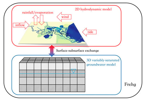
3.4. Surface-Subsurface Coupling
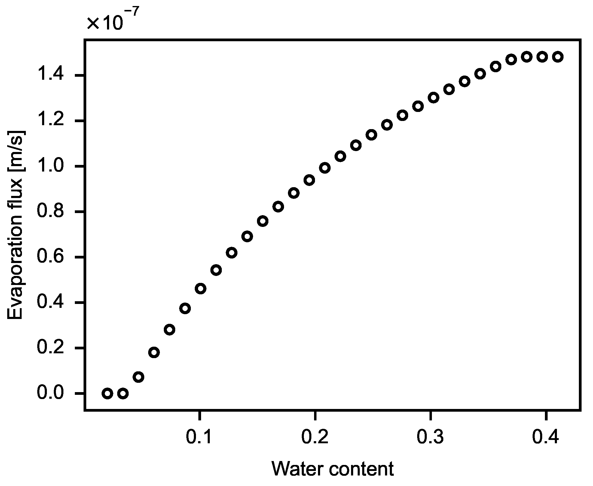
3.5. Rainfall and Evaporation
3.6. Thin-Layer Treatment
3.7. Comparing SWE and DW Models
4. Tests and Results
4.1. Overview
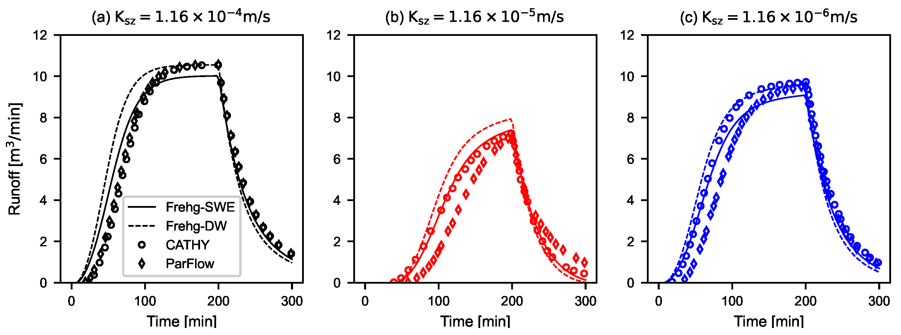
4.2. Rainfall on a Sloping Plane
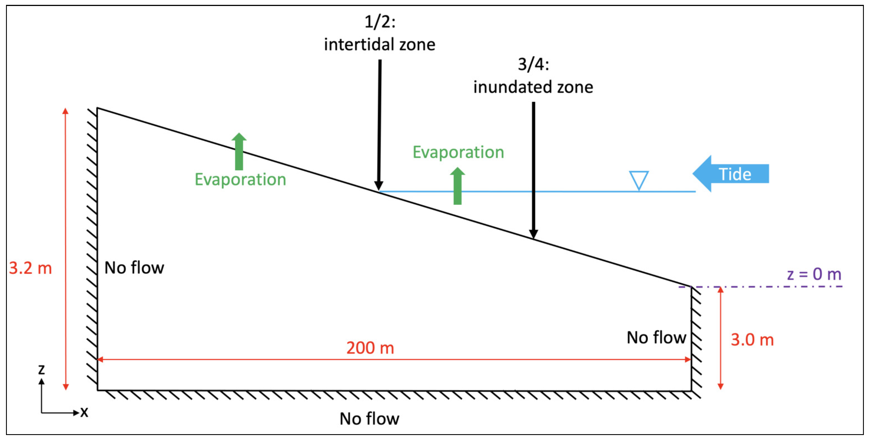
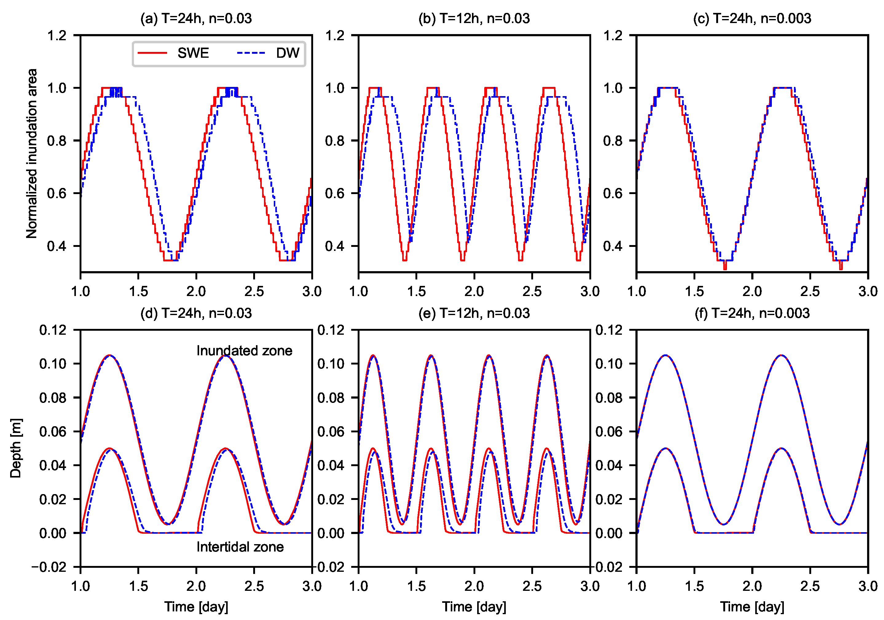
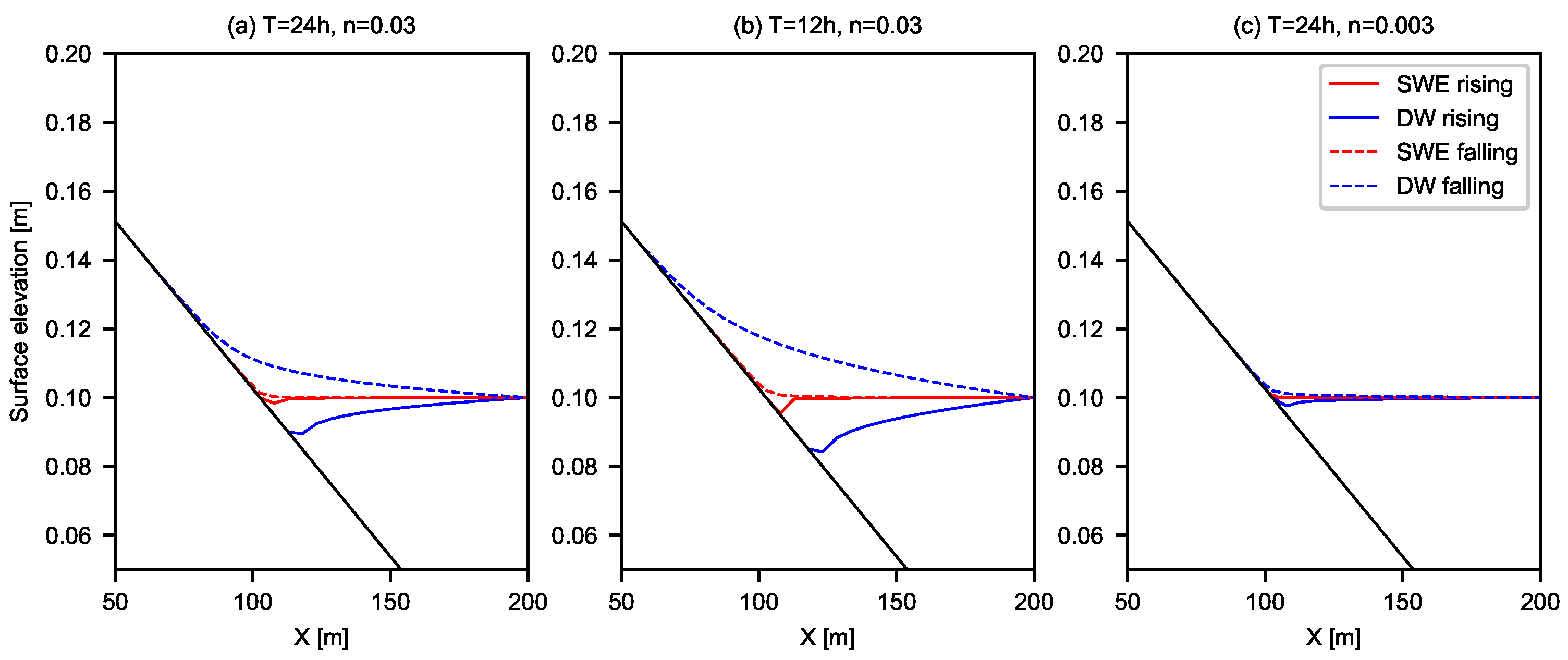
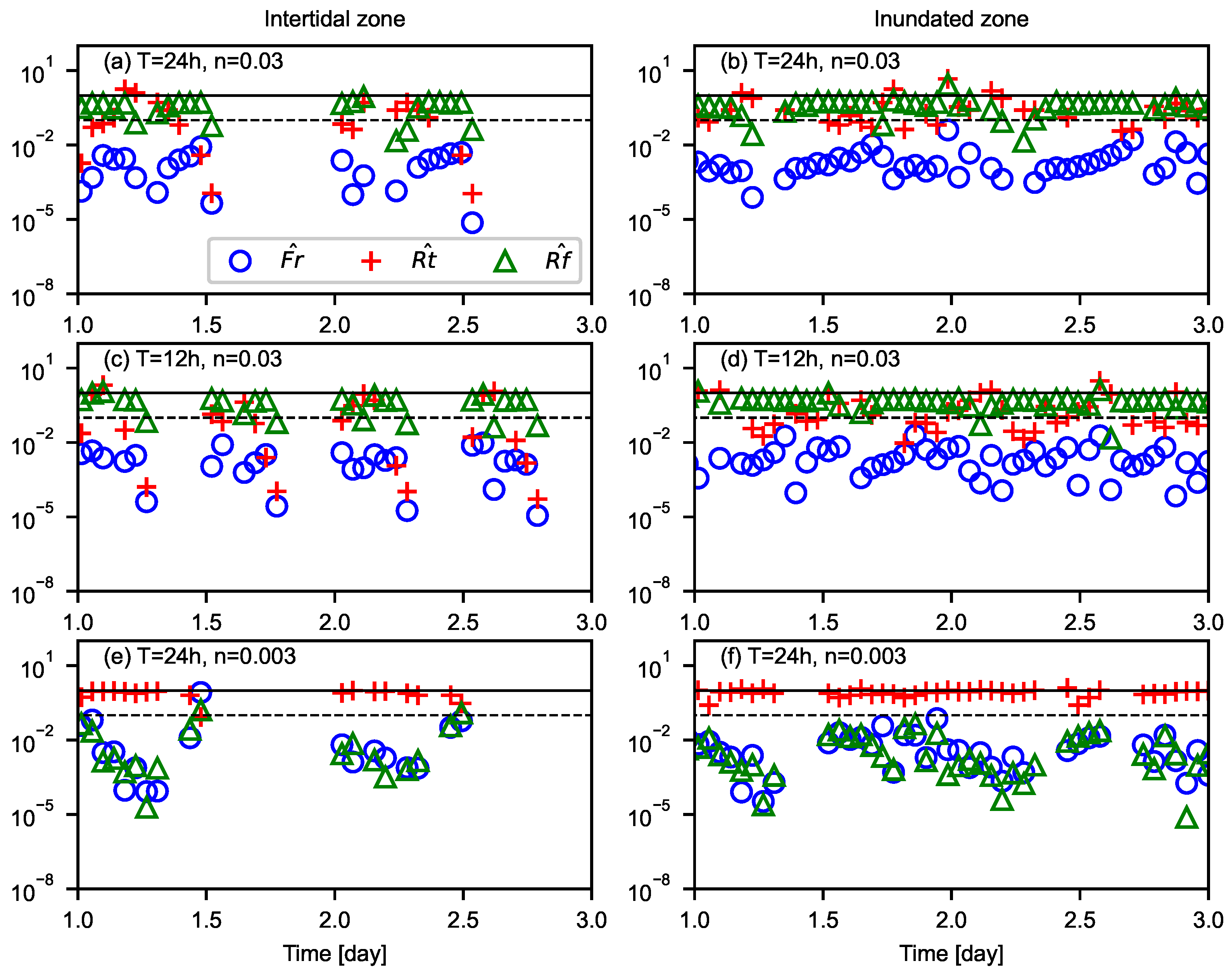
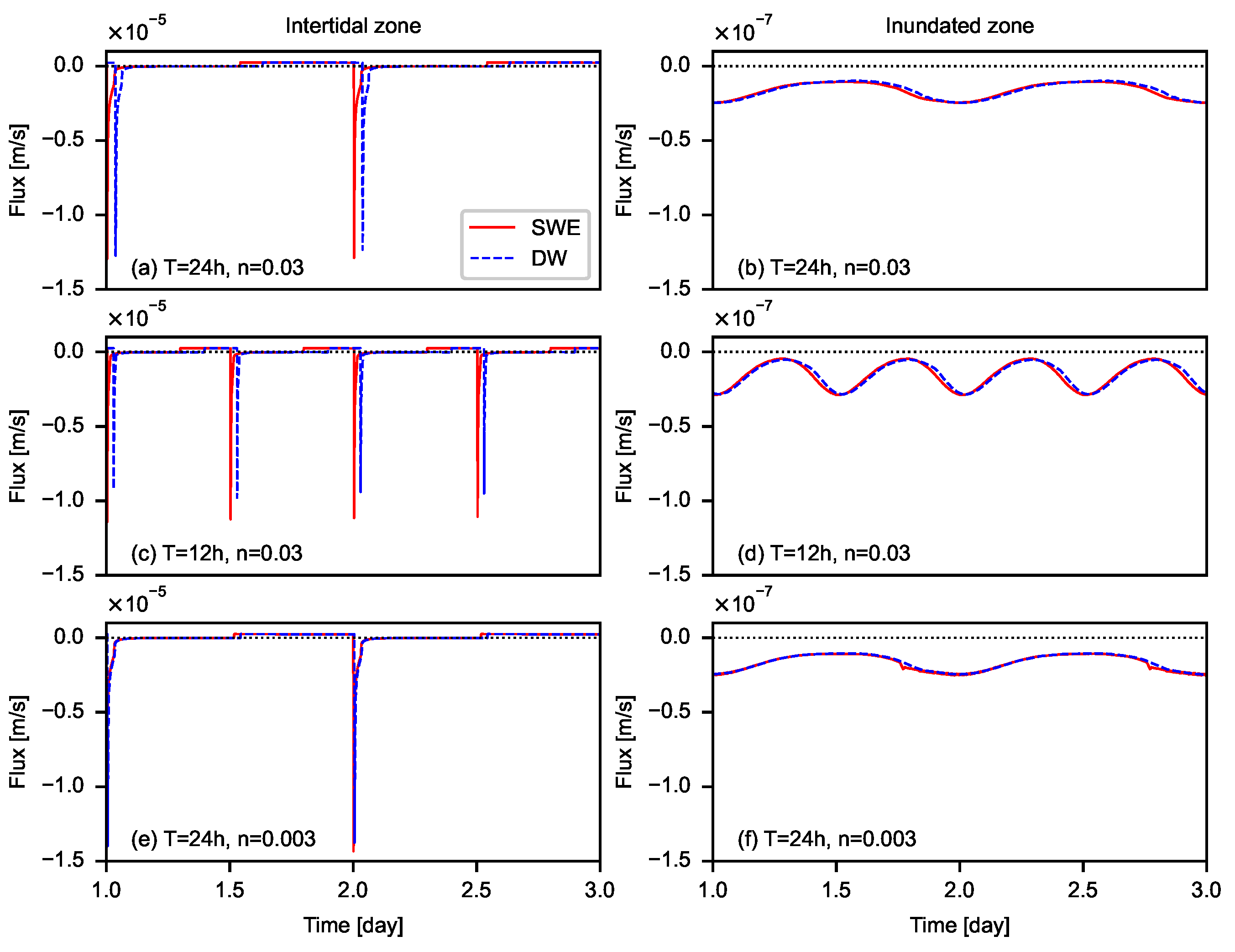
4.3. Inundation of an Intertidal Zone
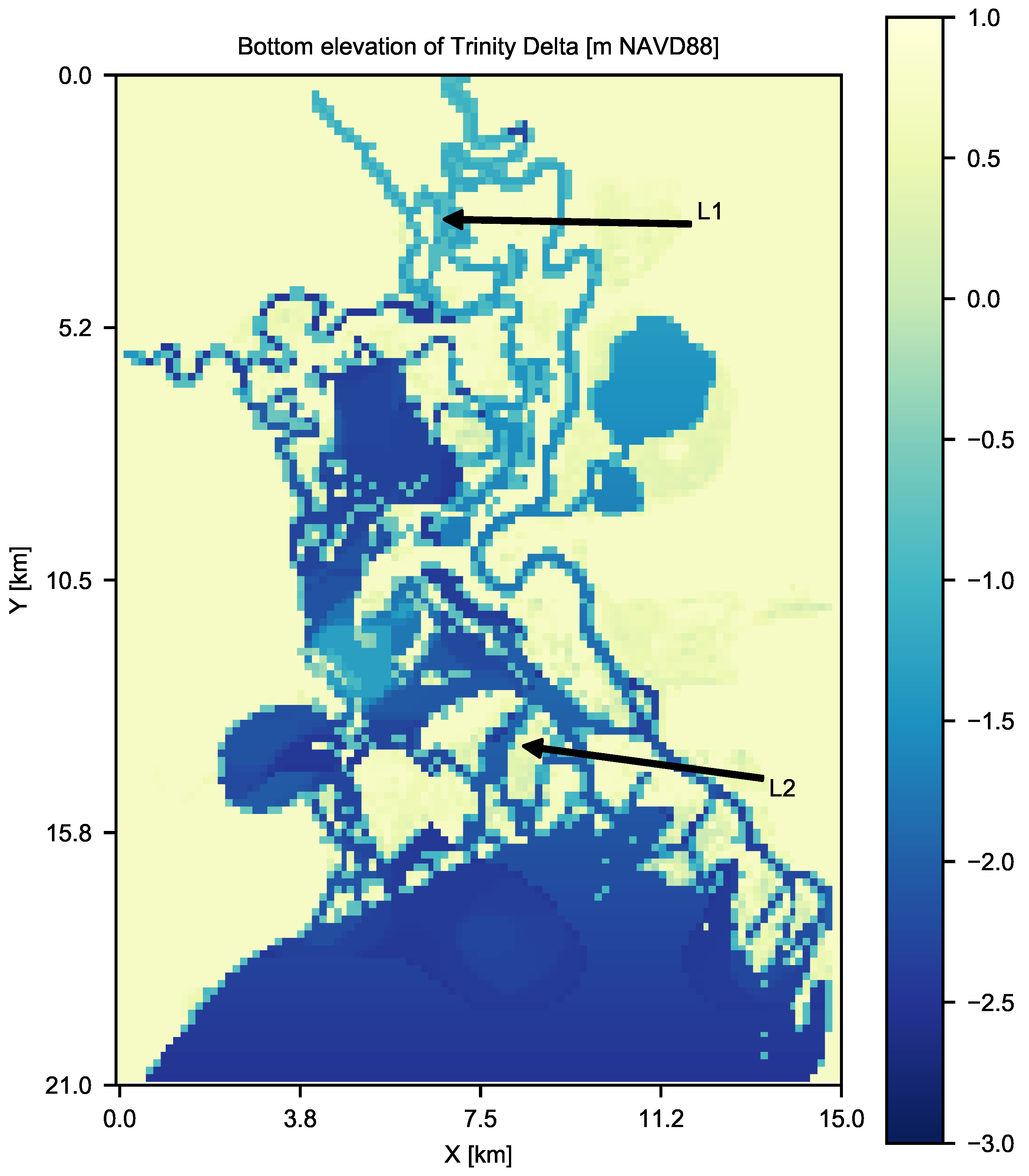
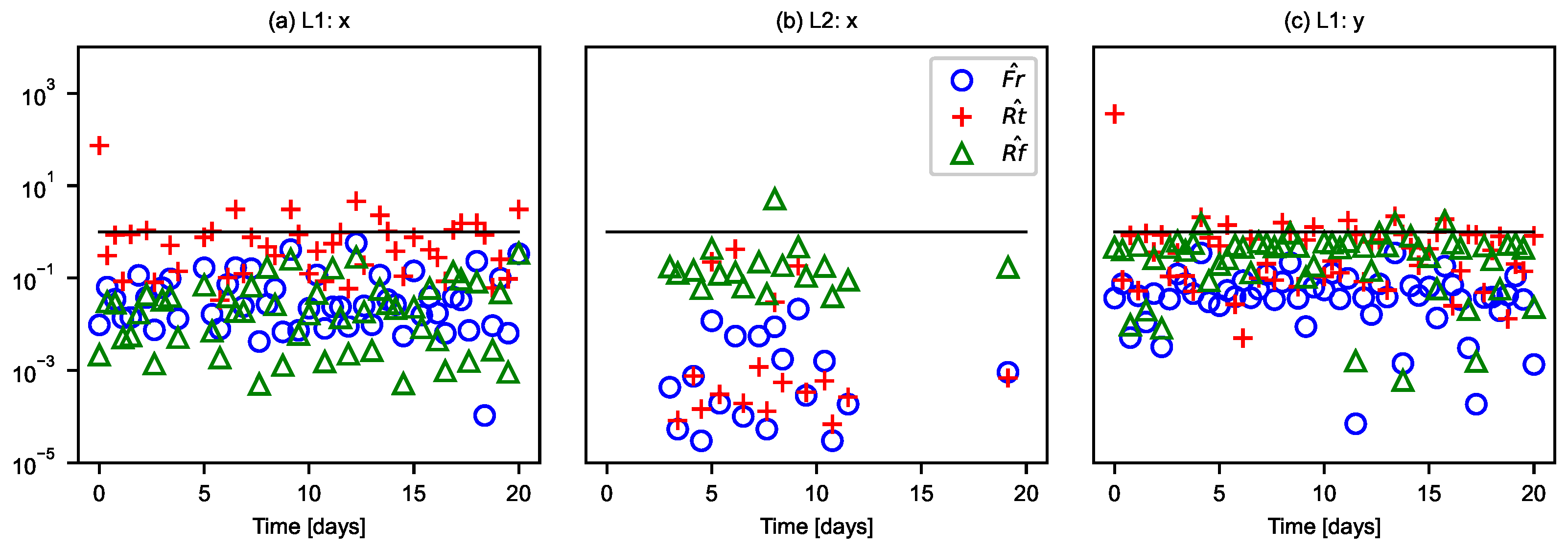
4.4. Surface-Subsurface Exchange in the Trinity River Delta
5. Discussion and Conclusions
Author Contributions
Funding
Institutional Review Board Statement
Informed Consent Statement
Data Availability Statement
Acknowledgments
Conflicts of Interest
Appendix A
References
- Inoue, M.; Park, D.; Justic, D.; Wiseman, W.J., Jr. A high-resolution integrated hydrology-hydrodynamic model of the Barataria Basin system. Environ. Model. Softw. 2008, 23, 1122–1132. [Google Scholar] [CrossRef]
- Matte, P.; Secretan, Y.; Morin, J. Hydrodynamic Modeling of the St. Lawrence Fluvial Estuary. I: Model Setup, Calibration, and Validation. J. Waterw. Port Coastal Ocean. Eng. 2017, 143. [Google Scholar] [CrossRef]
- Rayson, M.D.; Gross, E.S.; Fringer, O.B. Modeling the tidal and sub-tidal hydrodynamics in a shallow, micro-tidal estuary. Ocean. Model. 2015, 89, 29–44. [Google Scholar] [CrossRef]
- Abarca, E.; Karam, H.; Hemond, H.F.; Harvey, C.F. Transient groundwater dynamics in a coastal aquifer: The effects of tides, the lunar cycle, and the beach profile. Water Resour. Res. 2013, 49, 2473–2488. [Google Scholar] [CrossRef]
- Shen, C.; Jin, G.; Xin, P.; Kong, J.; Li, L. Effects of salinity variations on pore water flow in salt marshes. Water Resour. Res. 2015, 51, 4301–4319. [Google Scholar] [CrossRef]
- Xin, P.; Zhou, T.; Lu, C.; Shen, C.; Zhang, C.; D’Alpaos, A.; Li, L. Combined effects of tides, evaporation and rainfall on the soil conditions in an intertidal creek-marsh system. Adv. Water Resour. 2017, 103, 1–15. [Google Scholar] [CrossRef]
- Yang, J.; Graf, T.; Herold, M.; Ptak, T. Modelling the effects of tides and storm surges on coastal aquifers using a coupled surface-subsurface approach. J. Contam. Hydrol. 2013, 149, 61–75. [Google Scholar] [CrossRef] [PubMed]
- Yu, X.; Yang, J.; Graf, T.; Koneshloo, M.; O’Neal, M.A.; Michael, H.A. Impact of topography on groundwater salinization due to ocean surge inundation. Water Resour. Res. 2016, 52, 5794–5812. [Google Scholar] [CrossRef]
- Zhang, Y.; Li, W.; Sun, G.; Miao, G.; Noormets, A.; Emanuel, R.; King, J.S. Understanding coastal wetland hydrology with a new regional-scale process-based hydrological model. Hydrol. Process. 2018, 32, 3158–3173. [Google Scholar] [CrossRef]
- Li, Z.; Hodges, B.R. Model instability and channel connectivity for 2D coastal marsh simulations. Environ. Fluid Mech. 2019, 19, 1309–1338. [Google Scholar] [CrossRef]
- Langevin, C.; Swain, E.; Melinda, W. Simulation of integrated surface-water/ground-water flow and salinity for a coastal wetland and adjacent estuary. J. Hydrol. 2005, 314, 212–234. [Google Scholar] [CrossRef]
- Li, Z.; Ozgen, I.; Maina, F.Z. A mass-conservative predictor-corrector solution to the 1D Richards equation with adaptive time control. J. Hydrol. 2020, 592. [Google Scholar] [CrossRef]
- Hunter, N.M.; Bates, P.D.; Horritt, M.S.; Wilson, M.D. Simple spatially-distributed models for predicting flood inundation: A review. Geomorphology 2007, 90, 208–225. [Google Scholar] [CrossRef]
- Ponce, V.M.; Li, R.M.; Simons, D.B. Applicability of kinematic and diffusion models. J. Hydraul. Div. ASCE 1978, 104, 353–360. [Google Scholar] [CrossRef]
- Li, Z.; Hodges, B.R. On modeling subgrid-scale macro-structures in narrow twisted channels. Adv. Water Resour. 2020, 135. [Google Scholar] [CrossRef]
- Cea, L.; Blade, E. A simple and efficient unstructured finite volume scheme for solving the shallow water equations in overland flow applications. Water Resour. Res. 2015, 51, 5464–5486. [Google Scholar] [CrossRef]
- Neal, J.; Villanueva, I.; Wright, N.; Willis, T.; Fewtrell, T.; Bates, P. How much physical complexity is needed to model flood inundation? Hydrol. Process. 2011, 26, 2264–2282. [Google Scholar] [CrossRef]
- Caviedes-Voullieme, D.; Fernandez-Pato, J.; Hinz, C. Performance assessment of 2D Zero-Inertia and Shallow Water models for simulating rainfall-runoff processes. J. Hydrol. 2020, 584. [Google Scholar] [CrossRef]
- Yang, J.; Zhang, H.; Yu, X.; Graf, T.; Michael, H.A. Impact of hydrogeological factors on groundwater salinization due to ocean-surge inundation. Adv. Water Resour. 2018, 111, 423–434. [Google Scholar] [CrossRef]
- Kuan, W.K.; Xin, P.; Jin, G.; Robinson, C.E.; Gibbes, B.; Li, L. Combined effect of tides and varying inland groundwater input on flow and salinity distribution in unconfined coastal aquifers. Water Resour. Res. 2019, 55, 8864–8880. [Google Scholar] [CrossRef]
- Xiao, K.; Li, H.; Xia, Y.; Yang, J.; Wilson, A.M.; Michael, H.A.; Geng, X.; Smith, E.; Boufadel, M.C.; Yuan, P.; et al. Effects of tidally varying salinity on groundwater flow and solute transport: Insights from modelling an idealized creek marsh aquifer. Water Resour. Res. 2019, 55, 9656–9672. [Google Scholar] [CrossRef]
- Geng, X.; Boufadel, M.C. Impacts of evaporation on subsurface flow and salt accumulation in a tidally influenced beach. Water Resour. Res. 2015, 51, 5547–5565. [Google Scholar] [CrossRef]
- Tsai, C.W. Applicability of kinematic, noninertia, and quasi-steady dynamic wave models to unsteady flow routing. J. Hydraul. Eng. 2003, 129, 613–627. [Google Scholar] [CrossRef]
- Fu, Y.; Dong, Y.; Xie, Y.; Xu, Z.; Wang, L. Impacts of Regional Groundwater Flow and River Fluctuation on Floodplain Wetlands in the Middle Reach of the Yellow River. Water 2020, 12, 1922. [Google Scholar] [CrossRef]
- Sparks, T.D.; Bockelmann-Evans, B.N.; Falconer, R.A. Development and analytical verification of an integrated 2-D surface water—Groundwater model. Water Resour. Manag. 2013, 27, 2989–3004. [Google Scholar] [CrossRef]
- Farthing, M.W.; Ogden, F.L. Numerical solution of Richards’ equation: A review of advances and challenges. Soil Sci. Soc. Am. J. 2017, 81, 1257–1269. [Google Scholar] [CrossRef]
- Arico, C.; Nasello, C. Comparative analyses between the zero-inertia and fully dynamic models of the shallow water equations for unsteady overland flow propagation. Water 2018, 10, 44. [Google Scholar] [CrossRef]
- Hodges, B.R. A new approach to the local time stepping problem for scalar transport. Ocean. Model. 2014, 77, 1–19. [Google Scholar] [CrossRef]
- Hutschenreuter, K.L.; Hodges, B.R.; Socolofsky, S.A. Simulation of laboratory experiments for vortex dynamics at shallow tidal inlets using the fine resolution environmental hydrodynamics (Frehd) model. Environ. Fluid Mech. 2019, 19, 1185–1216. [Google Scholar] [CrossRef]
- Gross, E.S.; Koseff, J.R.; Monismith, S.G. Evaluation of advective schemes for estuarine salinity simulations. J. Hydraul. Eng. 1999, 125, 32–46. [Google Scholar] [CrossRef]
- Pareja-Roman, L.F.; Chant, R.J.; Ralston, D.K. Effects of locally generated wind waves on the momentum budget and subtidal exchange in a coastal plain estuary. J. Geophys. Res. Ocean. 2019, 124, 1005–1028. [Google Scholar] [CrossRef]
- Zheng, L.; Weisberg, R.H. Tide, buoyancy, and wind-driven circulation of the Charlotte Harbor estuary: A model study. J. Geophys. Res. 2004, 109. [Google Scholar] [CrossRef]
- Casulli, V. Semi-implicit finite-difference methods for the 2-dimensional shallow-water equations. J. Comput. Phys. 1990, 86, 56–74. [Google Scholar] [CrossRef]
- Casulli, V.; Cattani, E. Stability, accuracy and efficiency of a semi-implicit method for three- dimensional shallow water flow. J. Comput. Phys. 1994, 27, 99–112. [Google Scholar] [CrossRef]
- Hodges, B.R. Accuracy order of Crank-Nicolson discretization for hydrostatic free-surface flow. J. Eng. Mech. ASCE 2004, 130, 904–910. [Google Scholar] [CrossRef]
- Mualem, Y. A new model for predicting the hydraulic conductivity of unsaturated porous media. Water Resour. Res. 1976, 12, 513–522. [Google Scholar] [CrossRef]
- van Genuchten, M.T. A closed-form equation for predicting the hydraulic conductivity of unsaturated soils. Soil Sci. Soc. Am. J. 1980, 44, 892–898. [Google Scholar] [CrossRef]
- Kirkland, M.R.; Hills, R.G.; Wierenga, P.J. Algorithms for solving Richards’ equation for variably saturated soils. Water Resour. Res. 1992, 28, 2049–2058. [Google Scholar] [CrossRef]
- Lai, W.; Ogden, F.L. A mass-conservative finite volume predictor-corrector solution of the 1D Richards’ equation. J. Hydrol. 2015, 523, 119–127. [Google Scholar] [CrossRef]
- Li, Z.; Hodges, B.R. Modeling subgrid-scale topographic effects on shallow marsh hydrodynamics and salinity transport. Adv. Water Resour. 2019, 129, 1–15. [Google Scholar] [CrossRef]
- McMahon, T.A.; Peel, M.C.; Lowe, L.; Srikanthan, R.; McVicar, T.R. Estimating actual, potential, reference crop and pan evaporation using standard meteorological data: A pragmatic synthesis. Hydrol. Earth Syst. Sci. 2013, 17, 1331–1363. [Google Scholar] [CrossRef]
- Geng, X.; Boufadel, M.C. Numerical modeling of water flow and salt transport in bare saline soil subjected to evaporation. J. Hydrol. 2015, 524, 427–438. [Google Scholar] [CrossRef]
- Barton, I. A parameterization of the evaporation from nonsaturated surfaces. J. Appl. Meteorol. 1979, 18, 43–47. [Google Scholar] [CrossRef]
- Liu, S.; Mao, D.; Lu, L. Measurement and estimation of the aerodynamic resistance. Hydrol. Earth Syst. Sci. Discuss. 2006, 3, 681–705. [Google Scholar]
- Sulis, M.; Meyerhoff, S.B.; Paniconi, C.; Maxwell, R.M.; Putti, M.; Kollet, S.J. A comparison of two physics-based numerical models for simulating surface water–groundwater interactions. Adv. Water Resour. 2010, 33, 456–467. [Google Scholar] [CrossRef]
- Maxwell, R.M.; Putti, M.; Meyerhoff, S.; Delfs, J.; Ferguson, I.M.; Ivanov, V.; Kim, J.; Kolditz, O.; Kollet, S.J.; Kumar, M.; et al. Surface-subsurface model intercomparison: A first set of benchmark results to diagnose integrated hydrology and feedbacks. Water Resour. Res. 2014, 50, 1531–1549. [Google Scholar] [CrossRef]
- Wu, R.; Chen, X.; Hammond, G.; Bisht, G.; Song, X.; Huang, M.; Niu, G.; Ferre, T. Coupling surface flow with high-performance subsurface reactive flow and transport code PFLOTRAN. Environ. Model. Softw. 2021, 137, 104959. [Google Scholar] [CrossRef]
- Li, Z.; Hodges, B.R.; Passalacqua, P. Building the Trinity River Delta Hydrodynamic Model; Technical Report Submitted to TWDB Under Contract No. 1800012195; Texas Water Development Board: Austin, TX, USA, 2020. [CrossRef]
- Li, Z.; Hodges, B.R.; Passalacqua, P. Hydrodynamic Model Development for the Trinity River Delta; Technical Report Submitted to TWDB Under Contract No. 1600011928; Texas Water Development Board: Austin, TX, USA, 2017.
- Kim, J.; Warnock, A.; Ivanov, V.Y.; Katopodes, N.D. Coupled modeling of hydrologic and hydrodynamic processes including overland and channel flow. Adv. Water Resour. 2012, 37, 104–126. [Google Scholar] [CrossRef]


| Parameter | Value | Units |
|---|---|---|
| L | 800 | m |
| 0.0005 | – | |
| n | 0.01986 | m s |
| 0.4 | – | |
| 0.08 | – | |
| 1.0 | m | |
| 2.0 | – | |
| 80 | m | |
| 0.1 | m | |
| 2.0 | s | |
| m s | ||
| 200 | min | |
| 100 | min |
| Parameter | (1) | (2) | (3) | Units |
|---|---|---|---|---|
| m s | ||||
| 0.5 | 1.0 | 1.0 | m |
| Parameter | Value | Units |
|---|---|---|
| 5 | m | |
| 0.05 | m | |
| 0.001 | – | |
| 2.0 | s | |
| m s | ||
| m s | ||
| 30 | day | |
| 3 | day | |
| 0.1 | m |
| Parameter | (1) | (2) | (3) | Units |
|---|---|---|---|---|
| 0.03 | 0.03 | 0.003 | m s | |
| 24 | 12 | 24 | hour |
| Parameter | Value | Units |
|---|---|---|
| 150 | m | |
| 150 | m | |
| 0.25 | m | |
| 10.0 | s | |
| 30 | day | |
| 20 | day | |
| 0.3 | m | |
| 2.0 | m/s |
| Name | SWE | SWE + Evap | SWE + Evap + Wind | DW + Evap |
|---|---|---|---|---|
| Surface flow solver | SWE | SWE | SWE | DW |
| Evaporation | No | Yes | Yes | Yes |
| Wind | No | No | Yes | No |
Publisher’s Note: MDPI stays neutral with regard to jurisdictional claims in published maps and institutional affiliations. |
© 2021 by the authors. Licensee MDPI, Basel, Switzerland. This article is an open access article distributed under the terms and conditions of the Creative Commons Attribution (CC BY) license (http://creativecommons.org/licenses/by/4.0/).
Share and Cite
Li, Z.; Hodges, B.R. Revisiting Surface-Subsurface Exchange at Intertidal Zone with a Coupled 2D Hydrodynamic and 3D Variably-Saturated Groundwater Model. Water 2021, 13, 902. https://doi.org/10.3390/w13070902
Li Z, Hodges BR. Revisiting Surface-Subsurface Exchange at Intertidal Zone with a Coupled 2D Hydrodynamic and 3D Variably-Saturated Groundwater Model. Water. 2021; 13(7):902. https://doi.org/10.3390/w13070902
Chicago/Turabian StyleLi, Zhi, and Ben R. Hodges. 2021. "Revisiting Surface-Subsurface Exchange at Intertidal Zone with a Coupled 2D Hydrodynamic and 3D Variably-Saturated Groundwater Model" Water 13, no. 7: 902. https://doi.org/10.3390/w13070902
APA StyleLi, Z., & Hodges, B. R. (2021). Revisiting Surface-Subsurface Exchange at Intertidal Zone with a Coupled 2D Hydrodynamic and 3D Variably-Saturated Groundwater Model. Water, 13(7), 902. https://doi.org/10.3390/w13070902