Future Flood Hazard Assessment for the City of Pamplona (Spain) Using an Ensemble of Climate Change Projections

Abstract

Understanding how the design hyetographs and floods will change in the future is essential for decision making in flood management plans. This study provides a methodology to quantify the expected changes in future hydraulic risks at the catchment scale in the city of Pamplona. It considers climate change projections supplied by 12 climate models, 7 return periods, 2 emission scenarios (representative concentration pathway RCP 4.5 and RCP 8.5), and 3 time windows (2011–2040, 2041–2070, and 2070–2100). The Real-time Interactive Basin Simulator (RIBS) distributed hydrological model is used to simulate rainfall-runoff processes at the catchment scale. The results point to a decrease in design peak discharges for return periods smaller than 10 years and an increase for the 500- and 1000-year floods for both RCPs in the three time windows. The emission scenario RCP 8.5 usually provides the greatest increases in flood quantiles. The increase of design peak discharges is almost 10–30% higher in RCP 8.5 than in RCP 4.5. Change magnitudes for the most extreme events seem to be related to the greenhouse gas emission predictions in each RCP, as the greatest expected changes are found in 2040 for the RCP 4.5 and in 2100 for the RCP 8.5.

1. Introduction

In recent years, several studies have focused on the impact of climate change on the hydrological cycle. Understanding the impacts of future climate on river flood risks and water resources is important to plan effective adaptation strategies to manage the expected changes in extreme event risks [1]. Flood risks are generally connected to the intensity and frequency of rainfall events in urban areas either located downstream of small catchments or subject to pluvial floods. Several studies have shown an increase pattern in precipitation intensities and the number of extreme events in a warmer climate [2,3,4]. Therefore, flood risks can increase in urban areas in the future [5,6], imposing high costs to aquatic and terrestrial ecosystems, human societies, and the economy [7]. The Intergovernmental Panel on Climate Change (IPCC) [8] identified statistically significant increasing trends in the number of heavy precipitation events in some regions, claiming that the frequency of extreme precipitation events or the proportion of total rainfall of such events will likely increase in the 21st century over many areas of the globe due to anthropogenic influences that have contributed to the intensification of extreme precipitations at the global scale.

Nevertheless, such increasing frequency and magnitude of extreme rainfall events do not imply that the long-term statistical trends of flood peaks will be also increasing [9]. The expected impact of climate change on the water cycle can be analyzed by using two approaches. First, trend analyses of observations recorded in the past with a set of statistical models can predict what will happen in the future. Second, rainfall-runoff models that use climate projections as input data can extract the flood change signal predicted by climate models [10]. Regarding the spatial scales, while the first approach is usually applied to large-scale studies, the second usually regards either large or small and finer spatial resolutions, such as catchment scales.

The input data in the second approach consist in a combination of global climate models (GCMs) and regional climate models (RCMs). GCMs simulate the climate behavior under a set of given representative concentration pathways (RCPs). RCMs downscale such climate projections on a finer spatial scale. Indeed, it is necessary to reproduce rainfall projections with adequate spatial and temporal scales specially to force hydrological models for small and medium catchment areas [11]. An ensemble of RCMs and GCMs is preferred to a single climate model to remove potential biases in the outputs of RCMs or GCMs [12]. In climate change studies, the most usual emission scenarios are the RCP 4.5, with the peak of greenhouse gas emissions around 2040 and a decline in the rest of the century, and the RCP 8.5, with increasing greenhouse gas emissions throughout the 21st century [13].

Many studies have analyzed the expected changes in flood risks in Europe by using both trend analyses and hydrological models as described above [14]. Recent studies to identify large-scale trends in observed time series have shown that a changing climate in the last decades both increases and decreases European river floods [15]. The results depend mainly on the part of Europe that is considered. While southern and eastern Europe show negative trends in river floods, the northern part of Europe has increasing trends. Nevertheless, some studies that use climate projections in hydrological models point out that, on average, flood peaks with return periods above 100 years can double their frequency within three decades in Europe [16]. Other studies confirm the increasing trend for the 100-year flood, particularly in western and eastern Europe, though they found decreasing trends in northeastern Europe [17,18]. Several large-scale studies in Europe that use hydrological models differ in their results, as they consider different climate models, downscaling techniques, or bias-correction methods [19]. For instance, results regarding the future design rainfalls of the Iberian Peninsula obtained from studies with larger scales are conflicting. Indeed, some findings obtained at the European scale show an increase of river flood risks in Spain [20], though global scale studies show the opposite in the same area [21]. In addition, the results can be different for a given region even using the same scale. Hence, at the European scale, the results obtained for Spain by Rojas et al. [18] are in contrast with Alfieri et al. [16] and Roudier et al. [20]. This lack of agreement cannot be read easily by decision makers. An additional source of uncertainty that could affect all these studies is that RCMs cannot reproduce extreme rainfall events in the future adequately. Indeed, Herrera et al. [22] show that RCMs have a good agreement with the observed mean precipitation in Spain, though upper percentiles that represent the amount of total rainfall from extreme events are underestimated. Furthermore, large-scale studies cannot provide flood risk assessment under climate change conditions at the catchment scale, despite that the quantification of flood quantile changes in urban areas would be interesting for municipalities and urban planners. Moreover, large-scales studies are mainly conduct for the 100-year flood, though other return periods are not usually considered.

Consequently, several studies have considered the impact of climate change in smaller river catchments, avoiding the extrapolation of the results from large-scale studies. They evaluate the climate change impact on the water cycle with different objectives, as climate change can have implications in sustainable management of ecosystem services [23], daily, monthly, and yearly streamflow patterns [24], seasonal precipitation [25], or engineering hydraulic design [10]. Indeed, the use of RCMs in the Mediterranean area at the river basin scale also demonstrated that different parts of southern Europe could have problems related to water scarcity in the future, as precipitation will decrease by the end of the 21st century in the central part of Greece [25], and a reduction of water yield mainly forced by decreasing precipitations has been detected in the Taro river basin (Italy) [23]. In Spain, similar results have been found for the time period 2021–2050. In this case, they are mainly due to the increase in both maximum and minimum temperatures at the national scale [26].

Findings in flood quantile changes in small-scale studies either can differ from the results obtained in the same zone by large-scale studies or can have different change signals for all the considered climate models. For instance, Ducharne et al. [27] found that low-flow quantiles could decrease, and high-flow quantiles could not significantly change in the Seine and Somme catchments (France), where European scale studies found an increase of design discharge. Statistically significant changes could be neglected when the mean of the results of the different trends in the ensemble of regional climate models is used [28]. The uncertainty associated with the results is not due only to the downscaling techniques but also on hydrological models. There are several studies that analyze the ensemble of climate models with an ensemble simulation approach [27,29,30,31].

This study aims to quantify expected flood quantile variations under climate change conditions in Pamplona (Spain) using climate change projections and a distributed rainfall-runoff model. Expected variations in precipitation quantiles extracted from climate change projections in the Iberian Peninsula in a recent study [32] are used as input data of the Real-time Interactive Basin Simulator (RIBS) model [33,34]. The Arga River catchment located in northern Spain is considered as case study, as it is the main driver of the largest floods observed in recent years in the River Ebro [35]. In addition, Pamplona has suffered frequent fluvial floods in last decades. This study focuses on a single medium-sized basin and on a single distributed hydrological model, trying to minimize the uncertainties associated with the results. Rather than using an ensemble simulation approach, a part of the work is dedicated to conducting a statistical calibration of the RIBS distributed hydrological model to reduce the model uncertainty. Furthermore, this region has been also chosen because it shows low biases associated with the climate models in reproducing the annual maxima series in the control period. This study also aims to analyze the results of the 12 climate models to identify given climate models that always provide the greatest or smallest flood quantile changes in the future.

2. Methodology

The methodology, proposed to identify flood quantile modifications driven by climate change, is divided into five parts: description of the RIBS hydrological model (Section 2.1), calibration methodology of the RIBS model (Section 2.2), hydrological modeling to quantify flood peaks in the current scenario (Section 2.3), spatial distribution of the future design storms (Section 2.4), and flood quantile change quantification (Section 2.5).

2.1. RIBS Model

The Real-time Interactive Basin Simulator (RIBS) is a distributed hydrological rainfall–runoff model that is typically used for real-time application on medium-size river basins. RIBS requires the information in a raster format, in this case with a cell size of 50 m. A digital elevation model (DEM) is used to determine the flow direction and flow accumulation in each cell of the domain. The soil information is used to estimate the parameters in the Brooks–Corey equation (Equation (1)) to calculate the part of the rainfall depth that is transformed into runoff in each cell.

$$K_s\left(y\right)=K_{0n}{e}^{-fy}{\left(\frac{\theta -{\theta }_r}{{\theta }_s-{\theta }_r}\right)}^{\epsilon }$$

(1)

where K_s(y) is the saturated hydraulic conductivity (mm/h); K_0n is the saturated hydraulic conductivity at the soil surface in normal direction (mm/h); f is he saturated hydraulic conductivity decay in depth (mm⁻¹), y is the soil depth (mm); $\theta$ is the soil moisture content, ${\theta }_r$ is the residual soil moisture content; i.e., the minimum value under which the humidity cannot be extracted by capillary forces; ${\theta }_s$ is the saturated moisture content; and ε is the index of soil porosity [36]. The Brooks–Corey equation assumes that K_s(y) has a maximum value at the soil surface ($K_{0n})$ and then exponentially decrease in the normal direction in the soil depth $y$ with the parameter $f$.

When rainfall intensity exceeds the infiltration capacity of the soil, surface runoff is generated. Runoff is propagated in the domain through Equations (2) and (3). The catchment is divided into two parts based on a given flow accumulation threshold. Cells with flow accumulation values under such a threshold represent hillslopes in the model and have a runoff velocity equal to $v_h$. Cells with flow accumulation values over the threshold represent streams and have a water velocity equal to $v_s$. It is assumed that $v_s$ depends on the discharge in the catchment outlet with respect to a reference flow rate $Q_{ref}$ (Equation (2)).

$$v_s\left(t\right)=C_v{\left[\frac{Q\left(t\right)}{Q_{ref}}\right]}^r$$

(2)

where $v_s$ is the water velocity in streams (m/s); $C_v$ is a model parameter (m/s); $Q\left(t\right)$ is the discharge at the catchment outlet in time step t (m³/s); $Q_{ref}$ is a reference discharge (m³/s); and r is a model parameter. If $r$ equals 0, $v_s$ equals $C_v$, remaining constant throughout the simulation. If $r$ is greater than 0, $v_s$ is greater than the parameter $C_v$ when the discharge at the catchment outlet is higher than $Q_{ref}$. At a given time step, the velocity in hillslopes, $v_h$, is related to the velocity in streams, $v_s$, with the dimensionless parameter $K_v$ (Equation (3)).

$$K_v=\frac{v_s\left(t\right)}{v_h\left(t\right)}$$

(3)

Both velocities can be considered uniform in all the stream and hillslope cells at a given time step, as $v_s$ depends only on the discharge at the catchment outlet. More information about the RIBS model can be found in Mediero et al. [37] and Garrote and Bras [33,34]. The parameter $r$ in Equation (4) has been set equal to 0 to reduce the computational cost of the model, as the number of simulations with climate change scenarios is high. Therefore, velocity in streams ($v_s$) is always equal to $C_v$ in all the time steps. The model parameters that are considered during the calibration procedure are reduced to three: $f$ (Equation (1)), $C_v$ (Equation (2)), and $K_v$ (Equation (3)).

2.2. Calibration of the RIBS Model

The calibration procedure aims to find the model parameter values that minimize the errors between the model results and the observations of the real system that it is intended to represent [38]. Such errors in model simulations can be represented with Equation (4) [39].

$$Q\left(x,t\right)=M\left(\theta ,x,t\right)+\epsilon \left(\theta ,x,t\right)$$

(4)

where $Q\left(x,t\right)$ is the measured discharge in a given location $x$ at the time step $t$; $M\left(\theta ,x,t\right)$ is the modeled discharge that is obtained using a set of parameters $\theta$; and $\epsilon \left(\theta ,x,t\right)$ is the error in the same location and time step with a set of parameters $\theta$.

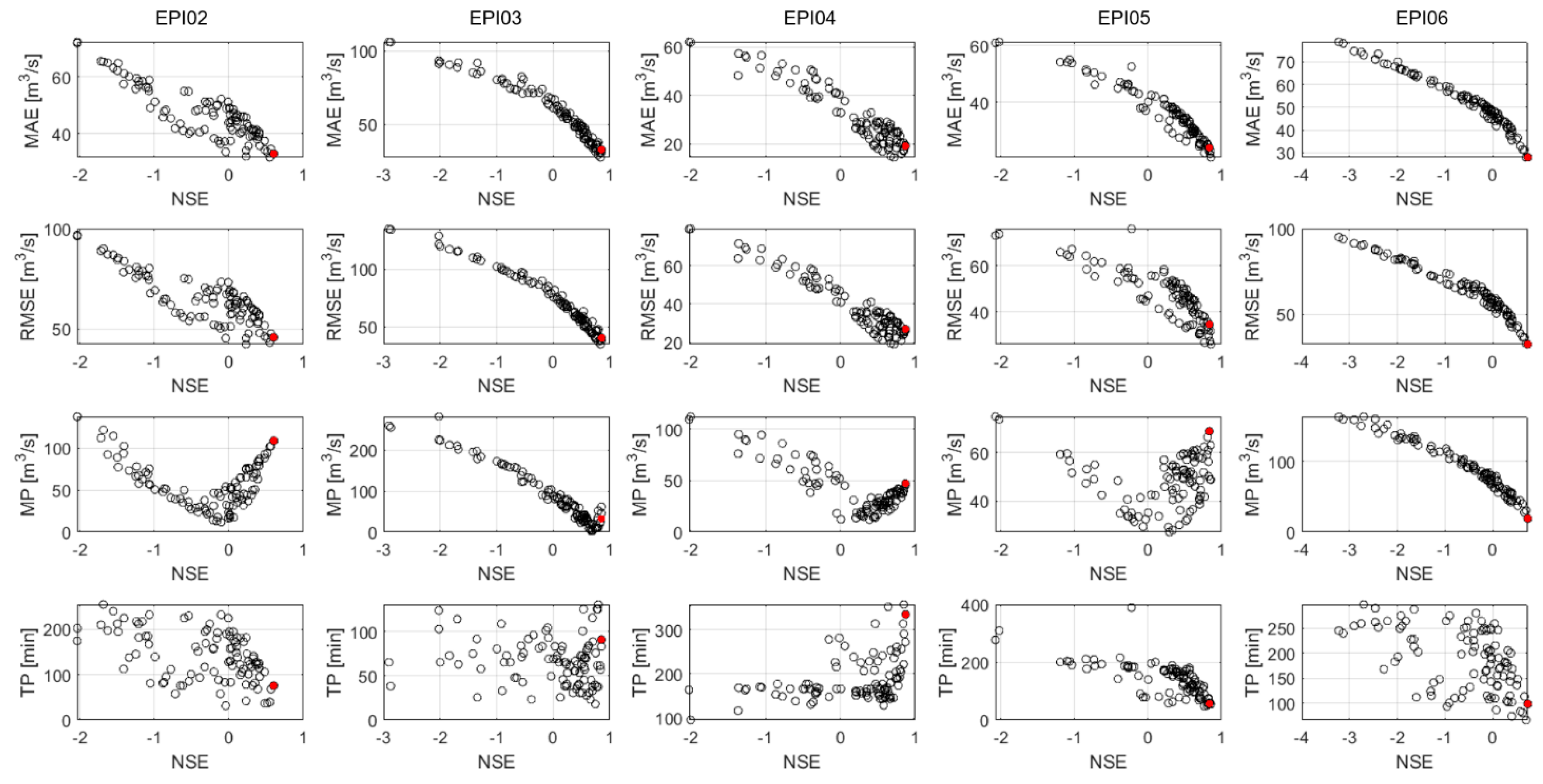
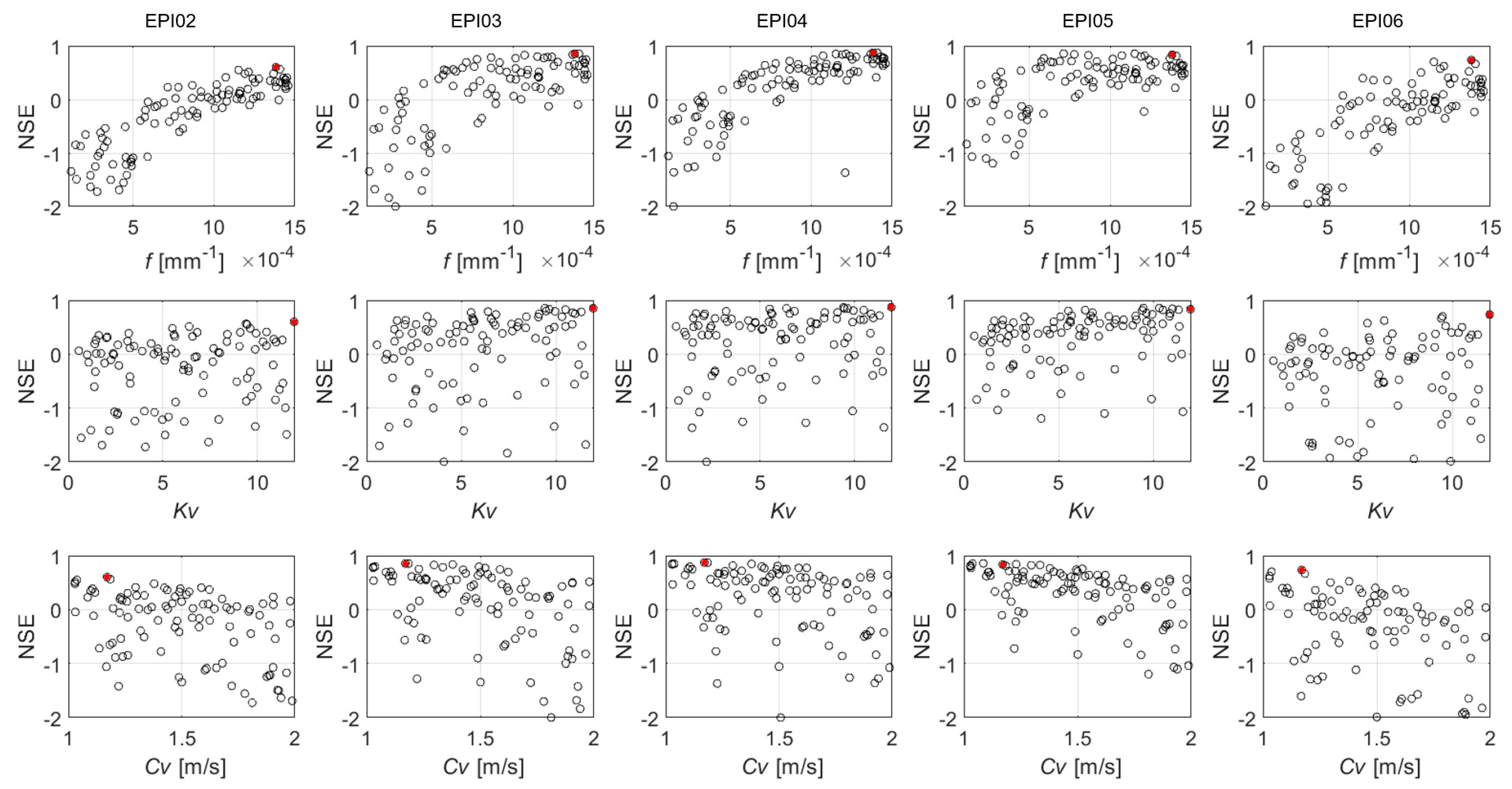
The model calibration can be based on optimization methods, seeking to minimize model errors. Model errors can be quantified by using different objective functions. A set of objective functions are needed to consider a set of aspects in the hydrograph, such as the hydrograph shape, the timing and magnitude of the peak and the magnitude of errors in low flows, among others.

In this study, five objective functions are used to calibrate the RIBS model. Three of them quantify the errors considering the complete hydrograph duration: mean absolute error (MAE), root mean square error (RMSE), and the Nash–Sutcliffe efficiency coefficient (NSE) (Equations (5)–(7)). Two additional parameters are considered to assess the fitting in the upper part of the hydrograph: time to peak (TP) and the magnitude of the peak (MP) (Equations (8) and (9)).

$$MAE\left(\theta \right)=\frac{1}{N}{{\displaystyle \sum }}_{k=1}^N\left|q_t-q_t^{\prime }\left(\theta \right)\right|$$

(5)

$$RMSE\left(\theta \right)=\sqrt{\frac{1}{N}{{\displaystyle \sum }}_{k=1}^N{\left(q_t-q_t^{\prime }\left(\theta \right)\right)}^2}$$

(6)

$$NSE\left(\theta \right)=1-\frac{{{\displaystyle \sum }}_{k=1}^N{\left(q_t-q_t^{\prime }\left(\theta \right)\right)}^2}{{{\displaystyle \sum }}_{k=1}^N{\left(q_t-\overline{q}\right)}^2}$$

(7)

$$TP\left(\theta \right)=\left|\mathrm{t}(\max \left(q_t\right))-\mathrm{t}\left(\max \left(q_t^{\prime }\left(\theta \right)\right)\right)\right|$$

(8)

$$MP\left(\theta \right)=\left|\max \left(q_t\right)-\max \left(q_t^{\prime }\left(\theta \right)\right)\right|$$

(9)

where $q_t$ is the measured discharge at a given time step $t$; $q_t^{\prime }\left(\theta \right)$ is the simulated discharge with a set of model parameters $\theta$ at the time step $t$; and $\overline{q}$ is the mean value of the observed discharges.

The NSE objective function [40] quantifies the improvement of using the simulated hydrograph compared with the average discharge of the observed hydrograph. The best value of all the objective functions is 0, except for NSE that supplies a value equal to one in a perfect match between the simulated and measured hydrographs. Indeed, MAE and RMSE values equal 0 and NSE values equal to 1 mean that there are not biases between the measured and the simulated discharge. A TP value equal to 0 means that the peak discharge of the simulated hydrograph occurs in the same time step as in the observed hydrograph. A MP value equal to 0 means that there is no difference between the magnitude of simulated and observed peaks.

2.3. Current Scenario

The design floods in the current scenario have been obtained by using the RIBS hydrological model with a set of design hyetographs as input data, obtained through an extreme frequency analysis. Daily observations at eight rain gauge stations have been considered. Both the GEV and the Gumbel distribution functions have been used to fit a frequency curve to annual maximum series. The return periods of 2, 5, 10, 50, 100, 500, and 1000 years are considered. An Areal Reduction Factor (ARF) is considered to reduce the mean areal precipitation in the catchment obtained from the precipitation quantiles estimated at rain gauge locations, as annual maximum rainfalls in the eight rain gauge stations are unlikely to occur on the same day in all the years.

The mean rainfall intensity for a given subdaily duration is obtained from the intensity–duration–frequency curve in the region. A storm duration of 24 h is considered. The 24 h design rainfall for a given return period is obtained by scaling a dimensionless hyetograph by the T-year daily rainfall multiplied by ARF. Therefore, the design hyetographs in the Arga River catchment have a fixed shape with the peak intensity in the central part of the event regardless the return period.

Finally, at-site rainfall precipitations at each time step given by the design hyetographs in the eight gauging sites are spatially distributed in the catchment, by using a grid with the cell size used by the RIBS model. The Thiessen polygon technique is used to obtain the precipitation fields in each time step. Therefore, 24 precipitation fields in the catchment are obtained for each design event, one for each time step of the hyetograph.

2.4. Climate Change Scenario

Expected changes in daily precipitation quantiles in the future under climate change conditions were extracted from rainfall climate projections supplied by 12 combinations of GCMs and RCMs (

Table 1. Ensemble of the 12 climate models considered in the analysis.

Code	Acronym	GCM	RCM
1	ICH-CCL	ICHEC-EC-EARTH	CCLM4-8-17
2	MPI-CCL	MPI-ESM-LR	CCLM4-8-17
3	MOH-RAC	MOHC-HadGEM2-ES	RACMO22E
4	CNR-CCL	CNRM-CM5	CCLM4-8-17
5	ICH-RAC	ICHEC-EC-EARTH	RACMO22E
6	MOH-CCL	MOHC-HadGEM2-ES	CCLM4-8-17
7	IPS-WRF	IPSL-CM5A-MR	WRF331F
8	IPS-RCA	IPSL-CM5A-MR	RCA4
9	MOH-RCA	MOHC-HadGEM2-ES	RCA4
10	ICH-RCA	ICHEC-EC-EARTH	RCA4
11	CNR-RCA	CNRM-CM5	RCA4
12	MPI-RCA	MPI-ESM-LR	RCA4

) of the EURO-CORDEX program [32]. Delta changes in daily precipitation quantiles are supplied for seven return periods (RP = 2, 5, 10, 50, 100, 500, and 1000 years), two representative concentration pathways (RCP 4.5 and RCP 8.5), and three time windows in the future (2011–2040, 2041–2070, and 2071–2100). A delta change represents the expected variation in rainfall quantiles for each combination of return period, climate model, time window, and RCP scenario. The delta changes are provided in a grid with a cell resolution of 0.11°. 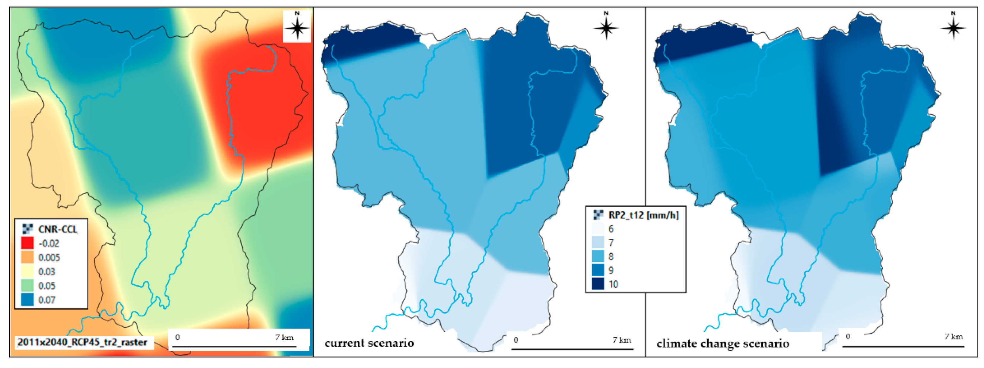Hence, the Arga River catchment is covered mainly by three points that have the greatest influence on the design rainfall variation, though additional seven points are also considered, as they cover smaller parts of the river catchment (Figure 1). Therefore, 504 values of delta changes are considered in each cell that are the possible combinations with the 7 return periods, 2 emission scenarios, 3 time windows, and 12 climate models considered in the study.

The delta changes are spatially distributed with the 50 m grid cell size that is used in the RIBS hydrological model simulations. Though the best geostatistical method depends on each case characteristics, ordinary kriging has been proved to provide better results than the inverse distance weighting (IDW) method in several studies regarding precipitation fields [41]. Nevertheless, in this case study the IDW technique has been used with a high exponent to maintain the same original squared shape of the delta changes. Furthermore, the use of the kriging method is not possible with these data as a fitting model cannot be determined for the semivariogram. Indeed, all the points have a fixed reciprocal distance. Therefore, for the same distance in the x-axis, there are several semivariance values in the y-axis that prevent any model from being able to converge (gaussian, exponential, and spherical).

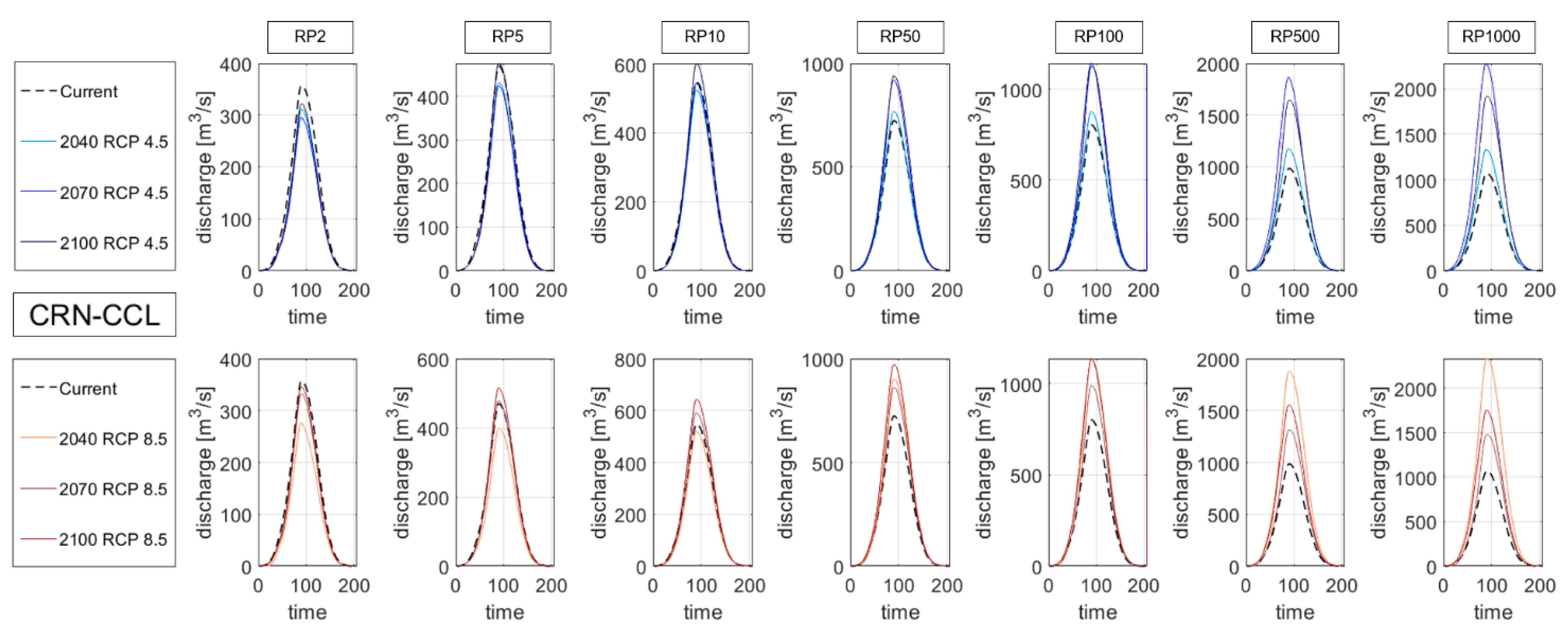
The spatial distributions of the future design precipitations are obtained combining the spatial distributions of both the current design rainfalls and the delta changes. Figure 1 shows the spatial distribution of the peak intensity in the 2 year hyetograph and the delta changes for the CNR-CCL climate model for the same return period in the 2040 time window. Considering the 504 combinations in each cell described above and the 24 time steps of the design hyetographs, a total of 12.096 rainfall spatial distributions have been considered as input data in the RIBS model.

2.5. Quantification of Expected Changes in Flood Quantiles

The expected changes in flood quantiles in the future are obtained from the comparison between flood quantiles in the future periods and the current period for each climate model. The flood quantile change supplied by a given climate model and return period (ΔQ_T) are obtained using the ratio between the hydrograph peak discharge in the climate change scenario ${\left(Q_p\right)}_{fut}$ and the hydrograph peak discharge in the current scenario ${\left(Q_p\right)}_{curr}$ (Equation (10)). ΔQ_T quantifies the change between a future time window and the current period, extracting the signal change supplied by a climate model forced with a given emission scenario, regardless the flood frequency curve obtained from observations. Therefore, the potential biases between the model simulations and observations do not have influence in the results.

$$\Delta Q_T=\frac{{\left(Q_{p,T}\right)}_{fut}}{{\left(Q_{p,T}\right)}_{curr}}$$

(10)

where (Q_p,T)_fut is the hydrograph peak magnitude for the return period T in the future period; (Q_p,T)_curr is the hydrograph peak magnitude for the return period T in the current period; and ΔQ_T is the expected change in the flood quantile for the return period T.

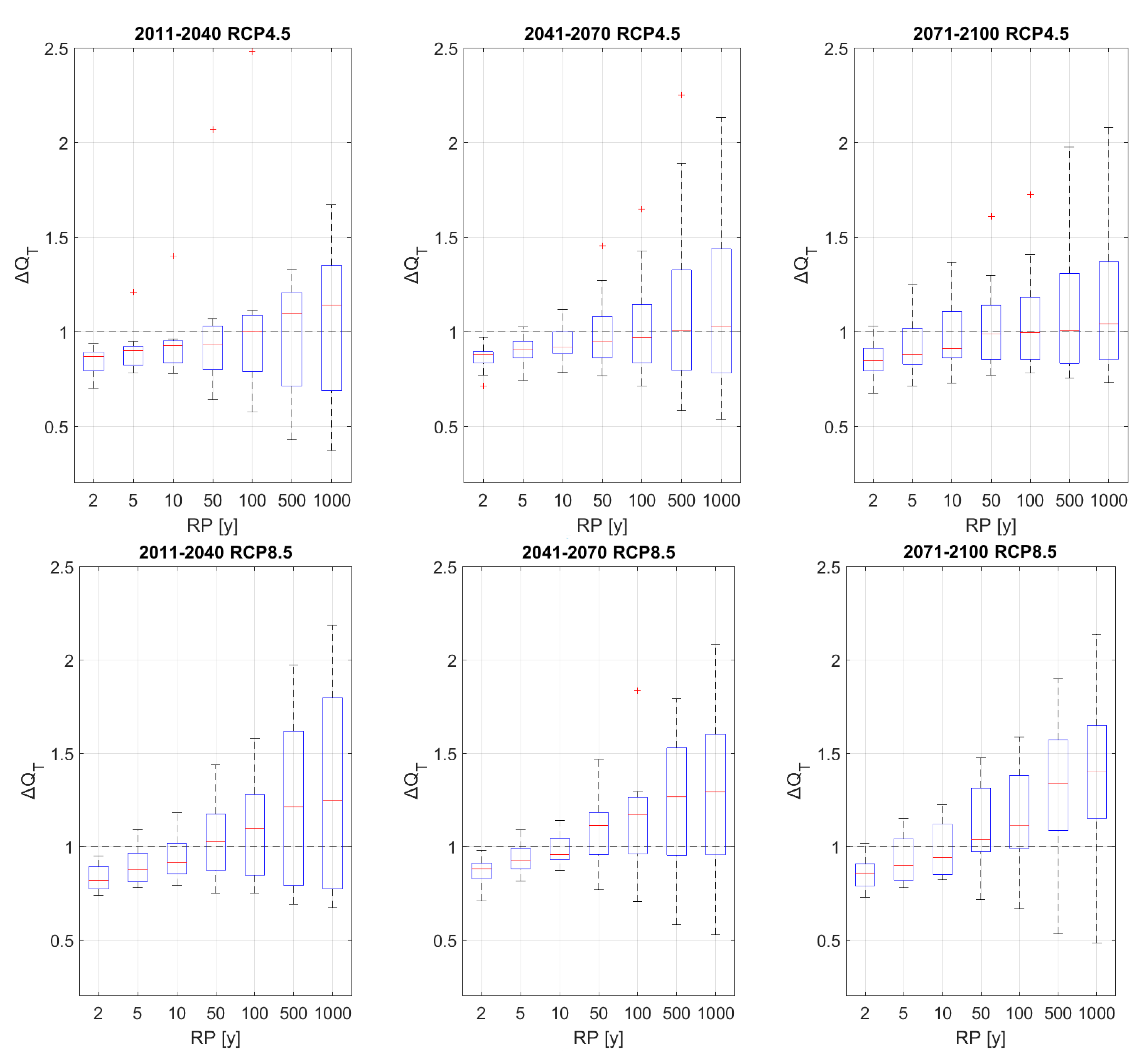
If ΔQ_T is greater than one, flood quantiles are expected to increase in the future. If ΔQ_T is smaller than one, flood quantiles are expected to decrease in the future. A value of one means that no changes in flood quantiles are expected in the future.

3. Data and Case Study

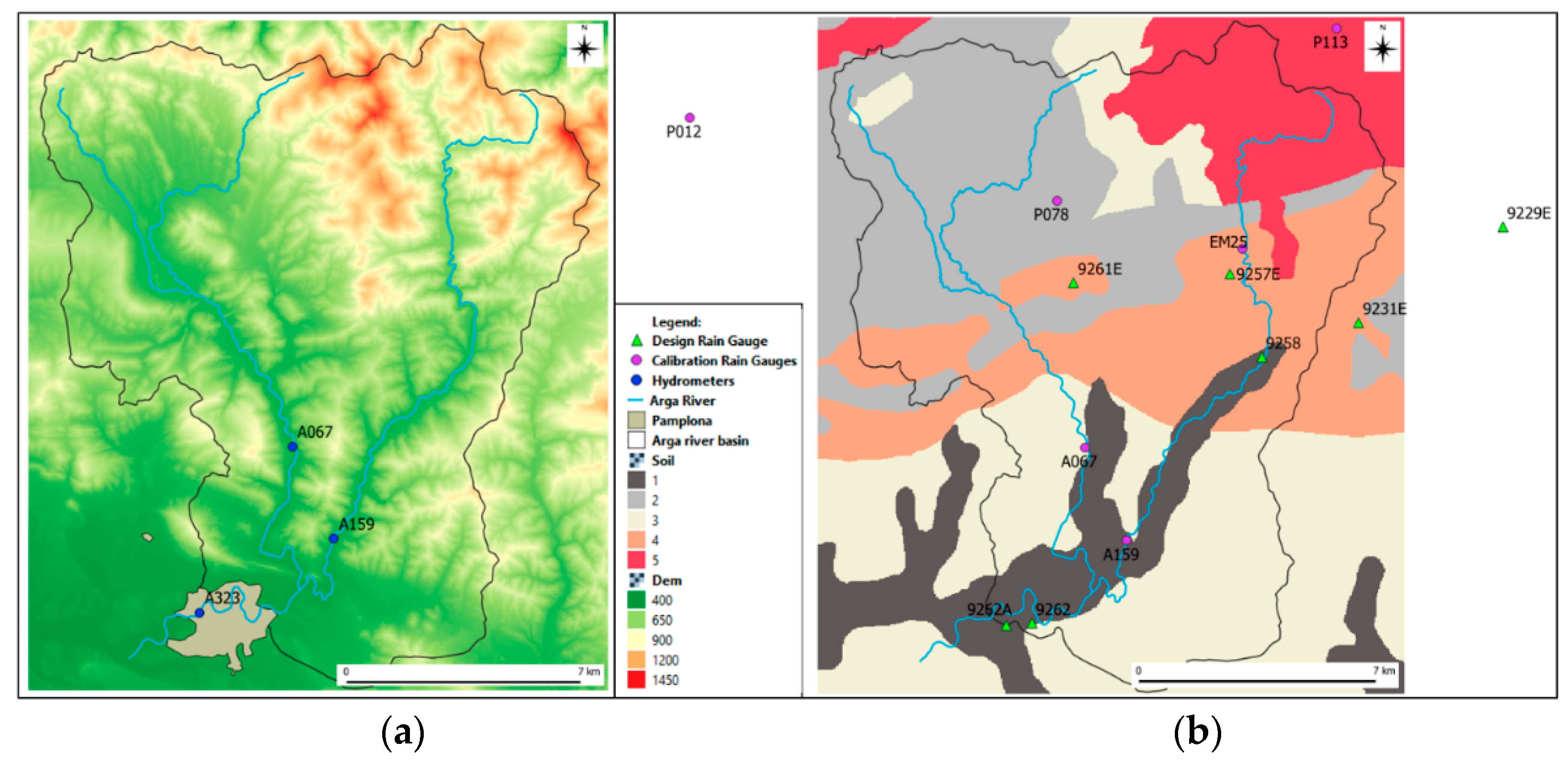
Pamplona is crossed by the Arga River that has a catchment area of 510 km². The Arga River is in the Navarre region and rises in the Urquiaga pass, located in the Paleozoic Quinto Real massif, one of the rainiest areas in Northern Spain. It is a tributary of Aragón River that has a total drainage area of 2759 km². In this study, the catchment outlet is located in the Pamplona city, where the A323 streamflow gauging station is placed, as shown in Figure 2.

Two types of rain-gauge stations are used in the study. For the RIBS model calibration procedure, six 15 min rain-gauge stations are used (purple circles in Figure 2). For estimating the design rainfall hyetographs, daily rain-gauge stations with longer time series are used (green triangles in Figure 2). Therefore, a time step of 15 min has been considered in the RIBS model simulations for both the calibration and the calculation with current and future design rainfalls.

Table 2. Summary about the rain- and streamflow-gauge stations considered in the study.

Code	Name	Instrument	Use	x (UTM)	y (UTM)	z (m asl)
A067	ULZAMA in OLAVE	Rain Gauge and Hydrometer	calibration	613,772	4,749,604	468
A159	ARGA in HUARTE	Rain Gauge and Hydrometer	calibration	615,717	4,745,302	454
A323	ARGA in PAMPLONA	Hydrometer	calibration	609,434	4,741,851	413
EM25	EMA DE EUGUI	Rain Gauge	calibration	621,072	4,758,771	628
P012	BERUETE	Rain Gauge	calibration	595,526	4,764,847	752
P078	LANTZ	Rain Gauge	calibration	612,505	4,761,016	645
P113	VALLE DE BAZTÁN	Rain Gauge	calibration	625,416	4,768,978	906
9229E	ESPINAL-AUZPERRI	Rain Gauge	design	633,099	4,759,795	870
9231E	ERRO	Rain Gauge	design	626,428	4,755,379	688
9257E	EUGUI ESTERIBAR	Rain Gauge	design	620,494	4,757,618	615
9258	ZUBIRI	Rain Gauge	design	621,945	4,753,786	536
9261E	OLAGUE	Rain Gauge	design	613,259	4,757,216	545
9262	PAMPLONA OBSERVATORIO	Rain Gauge	design	611,315	4,741,479	442
9262A	PAMPLONA INSTITUTO	Rain Gauge	design	610,148	4,741,399	441
9263I	ILUNDAIN	Rain Gauge	design	620,048	4,736,998	572

contains a summary about the streamflow- and rain-gauge station network.

The soil data were supplied by the Spanish National Geographic Institute IGN (Madrid, Spain), “Instituto Geográfico Nacional” in Spanish, in a shapefile format. The DEM was also supplied by IGN in a raster format. All the data in the RIBS model are provided in a raster format with a cell size of 50 m. Therefore, the soil raster in Figure 3 was obtained sampling the shapefile with a 50 m grid.

Table 3. Hydraulic characteristics of the soil classes belonging to the soil raster.

Soil Class	${\mathit{K}}_{0\mathit{n}}(\mathbf{mm}/\mathbf{h})$	${\mathit{\theta }}_{\mathit{s}}$	${\mathit{\theta }}_{\mathit{r}}$	$\mathit{\epsilon }$
1	50	0.5	0.04	3.5
2	1	0.35	0.04	3.5
3	25	0.25	0.03	3.5
4	15	0.3	0.03	3.5
5	30	0.25	0.01	6

reports the Brooks–Corey parameter values (see Section 2.1) for each soil class.

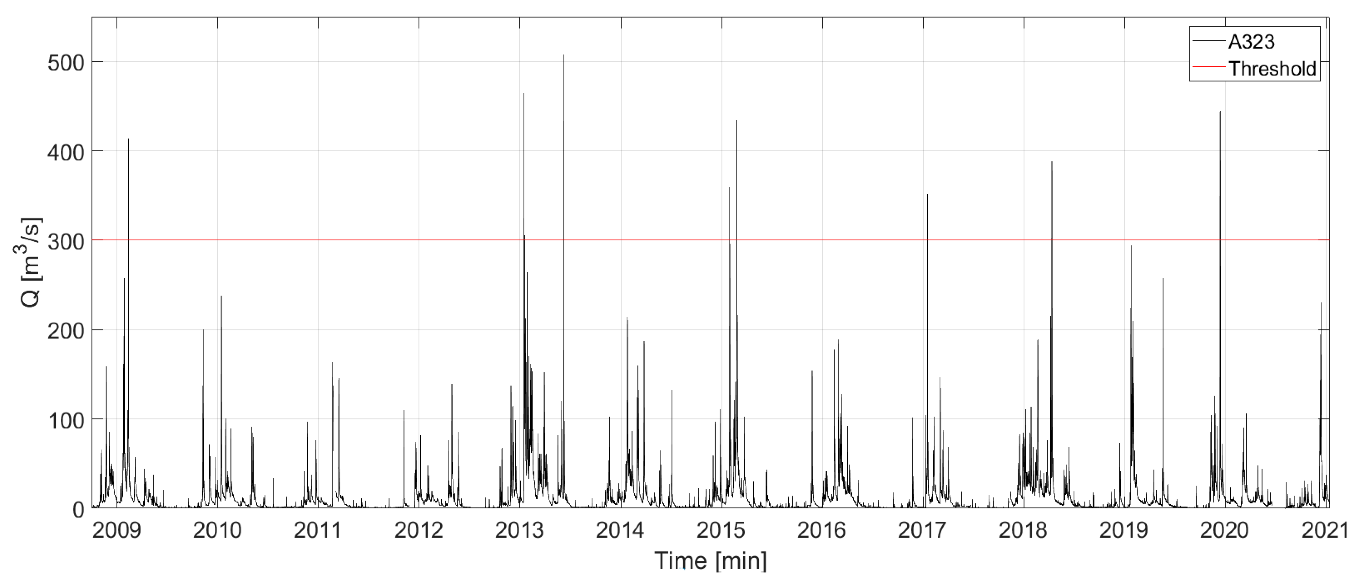
The greatest flood events of the Arga River in Pamplona in the last decade have been selected for the calibration of the RIBS hydrological model. A peak-over-threshold (POT) analysis has been applied to the streamflow time series recorded at the A323 hydrometer located at the catchment outlet. 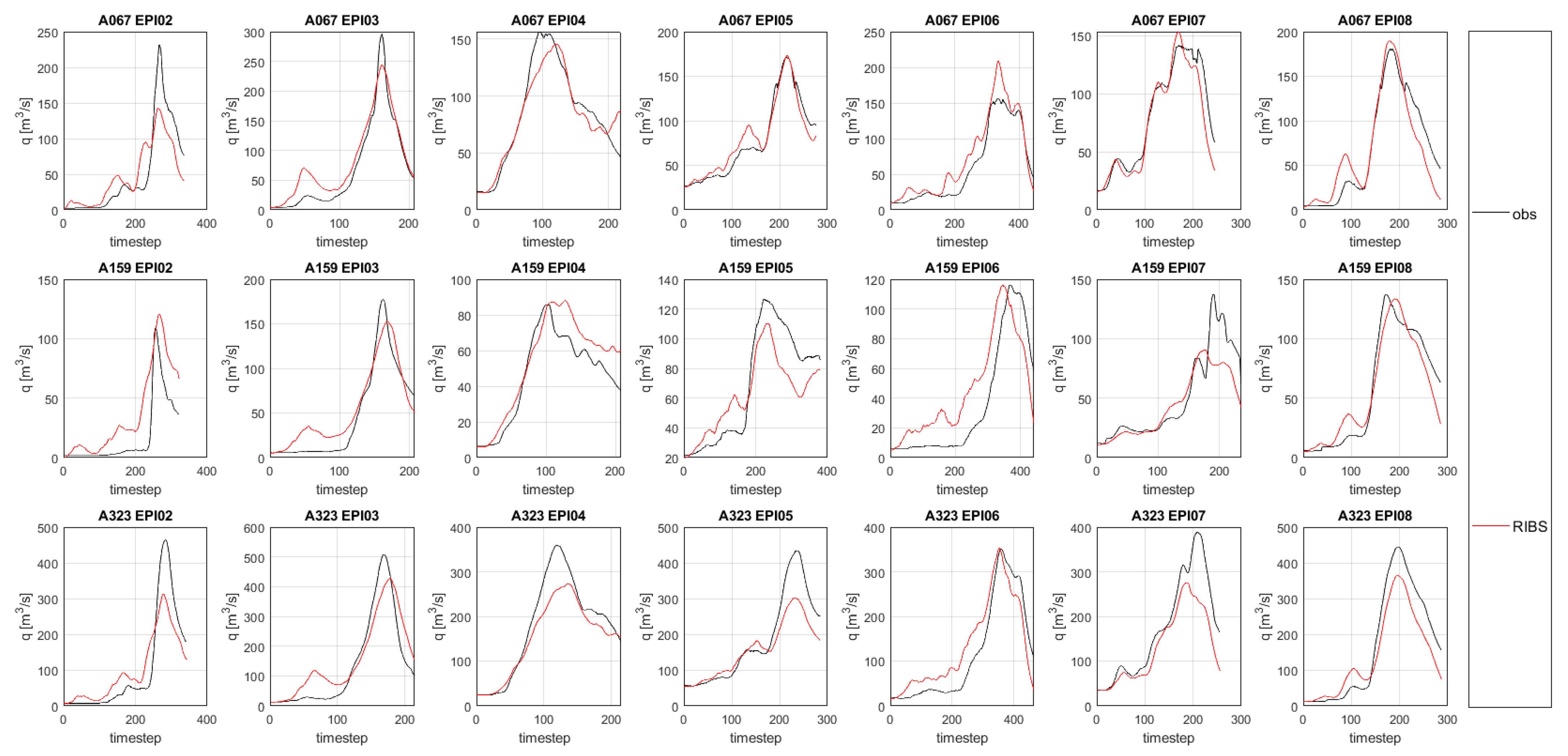A threshold of 300 m³/s has been considered, as floods that exceed such a threshold usually drive significant direct losses in the Pamplona city (Figure 3). Eight flood events have been selected for the calibration and validation methodology of the RIBS hydrological model. They are named from EPI01 to EPI08 in chronological order.

However, EPI01 has been removed from the calibration process, as two rain-gauge stations were out of service for this event. Hence, five events were used in the calibration procedure (EPI02, EPI03, EPI04, EPI05, and EPI06) and two in the validation (EPI07 and EPI08). A summary of the selected flood events is included in

Table 4. Summary of the flood events considered in the calibration process of the Real-time Interactive Basin Simulator (RIBS) model. Maximum intensity refers to the mean rainfall intensity in the catchment.

Code	Date	Flood Duration (h)	Maximum Intensity (mm/15 min)	Peak Flow (m3/s)
EPI02	12–17 January 2013	105	7.2	464.5
EPI03	7–10 June 2013	53	13.2	507.9
EPI04	29 January–3 February 2015	110	5.4	359.3
EPI05	23–27 February 2015	95	4.9	434.2
EPI06	12–17 January 2017	101	6.0	351.1
EPI07	10–12 April 2018	53	6.1	388.3
EPI08	11–13 December 2019	64	6.9	444.3

.

4. Results

In this section, the results of the hydrological simulation with the RIBS model are shown. First, the results of the calibration and validation methodology are reported. Second, the expected changes in flood quantiles in the future are compared with the design peak discharges in the current scenario.

4.1. RIBS Model Calibration and Validation

A set of 100 parameter value combinations generated randomly with a uniform distribution in the range of parameter values shown in

Table 5. Ranges of the RIBS model parameter values used in the calibration procedure.

Parameter	Lower Limit	Upper Limit
f (mm−1)	10−4	1.5 × 10−3
Cv (m/s)	1.0	2.0
Kv	0.5	12

has been considered in the calibration procedure.

The five objective functions selected in Section 2.2 have been calculated for the five flood events considered in the calibration process in the three hydrometers located in the Arga River catchment (A067, A159, and A323).

The model errors in the three streamflow-gauge stations have been combined using a weighted mean, to summarize the results of the calibration with a unique value for each flood event in the catchment. The results of the calibration process are shown in Figure 4. The 100 black circles in each subplot represent the simulations with the 100 combinations of parameter values. The red filled circle shows the model error of the best set of parameters used after the calibration in the flood quantile calculation.

Figure 4 shows that the parameter value combinations with the smallest values of the MAE and RMSE objective functions agree with the greatest values of the NSE objective function. However, a higher variability can be found in terms of the MP objective function, indicating that a good fit for the flood peak magnitude does not imply a good fit in the flood hydrographs shape. The results of the TP objective function indicate that it is not able to identify the best model parameter value combinations.

Nevertheless, the best combination of parameter values that minimize errors has been selected from the results of all the five objective functions. The set of parameter values that minimize the error has been identified for each flood event and each objective function. The best combination of parameter values has been selected analyzing the 25 parameter values. The objective function results for both the calibration and validation flood events with the combination of parameter values selected as calibration results are shown in

Table 6. Weighted values of the objective function values in the three hydrometers considered in the study for the events used in the calibration and validation phases. The results correspond to simulations with the RIBS model parameter values obtained in the calibration process.

Objective Functions	EPI02	EPI03	EPI04	EPI05	EPI06	EPI07	EPI08
RMSE (m3/s)	45.7	40.4	27.0	34.6	32.2	37.0	37.2
MAE (m3/s)	33.0	32.7	19.1	24.2	28.1	24.8	30.6
TP (min)	75	90	330	60	90	195	75
MP (m3/s)	108.9	61.3	47.2	68.9	19.3	67.4	43.4
NSE	0.60	0.85	0.87	0.86	0.74	0.82	0.87

.

Most of flood events show an NSE result higher than 0.8 that is a good fitting. The RMSE and MAE objective functions have small values when the NSE objective functions has high values, indicating that the three objective functions can identify the best parameter values. In terms of the TP objective function, most of flood events show values below 1.5 h that can be considered a good fit. The mean value of the observed flood peaks in the calibration is 420 m³/s, and the mean value of the MP objective function is 50 m³/s that corresponds to an error of 12%.

Figure 5 shows the relationship between the NSE objective function and the RIBS parameter values. The parameter values selected in the calibration and used for model validation is shown in red. NSE shows a higher sensitivity to the parameter f. Indeed, different values of f can correspond to different values of flood volume, and there is only one value that is optimal for the model. The RIBS model is less sensitive to the parameters $K_v$ and $C_v$, as the catchment time of response depend on water velocities in hills and streams that can be obtained with several combinations of $K_v$ and $C_v$. Nevertheless, the best set of parameter values identified in the calibration process is always in the upper part of the graphs, indicating its goodness of fit. The parameter values selected in the calibration process are included in

Table 7. RIBS parameter values for the best combination identified in the calibration process.

Parameter	f (mm−1)	Cv (m/s)	Kv
Optimal value	1.4 × 10−3	1.17	11.9

.

Figure 6 shows the comparison between the observed and simulated hydrographs, considering the set of model parameter values selected in the calibration process. The results of the calibration show that the simulated hydrographs are closer to the observed hydrographs at the A067 streamflow-gauging station rather than in the other hydrometers. The location of such a hydrometer pointed to a higher reliability in discharge estimations from water level measurements. Therefore, the results of the calibration process confirm the higher reliability of the A067 streamflow-gauging site. Errors in the A159 hydrometer can be driven by flood control processes in the Eugui reservoir located upstream in the Arga River. Underestimation in the RIBS model simulations in the EPI07 event could be explained by flood control processes and flow releases in such a reservoir, as the second rising limb of the observed hydrograph seems not to be forced by rainfall.

In the two validation flood events (EPI07 and EPI08), a good fitting between the observed and simulated hydrographs can be seen, mainly in the A067 hydrometer and in the A159 and A323 streamflow-gauging stations for the EPI08 flood event. In the EPI07 flood event, the simulated hydrograph underestimates the observed hydrograph in the A159 gauging site that could be due to the Eugui dam. Therefore, the simulation also underestimates the observed hydrograph in the A323 gauging stations which is located downstream the A159.

4.2. Flood Quantile Changes Expected in the Future

Flood quantile changes are quantified in the streamflow-gauging site A323 located at the river basin outlet of the Arga River catchment in the Pamplona city. The flood quantiles in the current scenario agree with the flood frequency curve obtained in the A323 hydrometer in the CAUMAX study [42], confirming the goodness of the model calibration. A comparison between flood quantiles in the future periods and the current period for each climate model has been carried out. Figure 7 shows the results for the CNR-CCL climate model. The figures for the rest of climate models are provided in the Supplementary Materials (Figures S1–S11).

The results for the CNR-CLL show a general increase of the flood quantiles in all the return periods, time windows and emission scenarios. Nevertheless, the results for all the climate models considered in the study are summarized to reduce potential biases in the future flood quantile estimates.

Expected changes in flood quantiles (ΔQ_T) are quantified for each climate model and return period with Equation (10). The results of the 12 climate models are summarized in a box plot for each return period, emission scenario, and future period (Figure 8). In the boxplots, the median value for the 12 climate models is highlighted by a red line, the horizontal black dashed line represents a value of one for ΔQ_T that separates the figure between the upper part with increasing flood quantiles and the lower part with decreasing flood quantiles.

Figure 8 uses the same vertical scale in each subplot. Therefore, the results for the three time windows and two RCPs can be compared. In RCP 4.5, a clear decrease in flood quantiles for the most frequent floods (2-, 5-, and 10-year return periods) is found for the three time windows in the future. The same signal of change for the most frequent floods is also visible in RCP 8.5 (lower boxplots of Figure 8). The dispersion of the results for the 12 climate models increases with the return period, showing the increasing uncertainty associated with the highest return periods. Nevertheless, in the RCP 8.5 the uncertainty for return periods greater than 50 years is smaller in the 2041–2070 and 2071–2100 time windows than in the period 2011–2040, with an evident increase of the design discharges. For return periods higher than 100 years, increasing flood quantiles are only found in the time window 2011–2040 for RCP 4.5. For RCP 8.5, higher positive changes are expected in the three time windows with flood quantiles increases higher than 25% for the 500- and 1000-year return period in the three time windows.

In addition, Figure 9 shows the results for the two RCP scenarios together reporting only the median values of the boxplots of Figure 8. A given color is used for each time window: cyan for 2011–2040, blue for 2041–2070, and black for 2070–2100. Dotted lines represent the results for RCP 4.5 scenario and solid lines for the emission scenario RCP 8.5.

Figure 9 shows the results for the median values of ΔQ_T values for each return period. The decrease in flood quantiles for the most frequent flood peaks (return periods smaller than 10 years) is also clear in this figure in the three time windows and both RCPs. Nevertheless, in this case a slight increase in the higher return periods (500 and 1000 years) is also evident for the RCP 4.5 in the three time windows, especially for the 2011–2040 period. For the highest return periods, RCP 8.5 leads to an increase in the 1000-year flood quantile 35% greater than in the RCP 4.5. In addition, RCP 8.5 points to 1000-year flood quantile increases of 40% compared with the current period.

However, the most interesting findings in Figure 9 are:

• The 100-year flood quantiles are expected to increase 10% in the RCP 8.5 already in the 2011–2040 time window;
• Flood quantile increases are generally greater in the scenario with higher emissions (RCP 8.5) than in the scenario with smaller emissions (RCP 4.5), except for the most frequent floods (2, 5, and 10 years) in the time window 2011–2040;
• Flood quantile increases of the most extreme events (500 and 1000 years) seem to be correlated with the greenhouse gas emission trend, as flood quantile increases in the RCP 4.5 scenario are expected to have their peak around 2040 with a subsequent decline, similar to the emission temporal evolution, and flood quantiles increase throughout the century with highest values in the 2100 in RCP 8.5, similar to the emission temporal evolution.

4.3. Influence of the GCMs and RCMs in the Flood Quantile Determination

Figure 10 shows the median values of ΔQ_T considering the three periods in the future, grouped by return periods and both GCMs and RCMs, to understand how given global or regional climate models have influence in the results. Therefore, the three time windows and two RCP scenarios are combined in a unique plot and each climate model has at least six values of ΔQ_T values for a given return period. The plot for GCMs does not show information about RCMs used to downscale their results. In addition, the plot for RCMs does not show information about the GCM from which they downscale the results.

While the ICH and MOH GCMs have been used three times, the rest of GCMs have been used twice. Therefore, in the left part of Figure 10 ICH and MOH medians are calculated with 18 values and the rest with 12 values. Regarding the RCMs, RCA points represent 30 values, CCL 24 values, RAC 12 values, and WRF just 6 values.

Figure 10 shows that climate models show differing influences on the results. GCMs may have a greater impact on the results compared with RCMs. While the CNR and IPS climate models point to a clear general increase of peak flow quantiles in the future, a similar tendency is shown only by the CCL RCM. Though the results of WRF seems to lead to a clear increase in the higher return periods, it is used only once to downscale the IPS climate model. Therefore, the increase is driven by the IPS GCM. On the contrary, CCL has a clear increasing tendency of peak flow quantiles for large return periods, and the results are more reliable than for the WRF RCM. In this case, the increasing trend is not driven by a given climate model, as it is used to downscale four different GCMs.

The RAC RCM is the only model that shows a slightly declining trend. Nevertheless, the influence of the GCMs that are combined with RAC seems to have a great influence on the results also in this case, as RAC is combined with MOH and ICH, which are the GCMs with milder slopes in the left part of Figure 10.

Figure 11 shows the median value of ΔQ_T for each combination of GCM and RCM, considering the three future time windows and the two RCPs. Therefore, also in this case each climate model has six values. The variability around the median values increase with the return periods, as was also shown in the boxplots of Figure 8. Nevertheless, variability patterns differ among climate models, and they seem to be driven by the GCMs. For instance, Figure 11 shows that the greatest increases are obtained with the CNR-RCA climate model, though RCA RCM does not show an increasing trend in Figure 10. Moreover, the influence of GCMs in the results can be seen analyzing the 1000-year flood results for the combinations that use the RCA RCM. The results vary depending on the GCM that is downscaled: CNR-RCA has a large variability and increase (red squares), MPI-RCA shows no significant changes (purple squares), and ICH-RCA presents an evident decrease in flood quantiles (blue squares).

5. Discussion and Conclusions

An analysis of the expected changes in flood quantiles in the future for Arga River in the city of Pamplona has been carried out using precipitation projections supplied by 12 climate models of the EURO-CORDEX program. Delta changes in daily rainfall quantiles obtained in a previous study have been used as input data in the RIBS distributed hydrological model to transform the expected changes in precipitation quantiles into changes in flood quantiles.

For this reason, the RIBS hydrological model has been calibrated with the seven greatest flood events in the city of Pamplona in the last decade. The results of calibration and validation show that the simulated hydrographs have a good fit with the observations, obtaining acceptable residual model errors both in terms of hydrograph shape (RMSE, MAE, NSE) and flood peak (TP, MP).

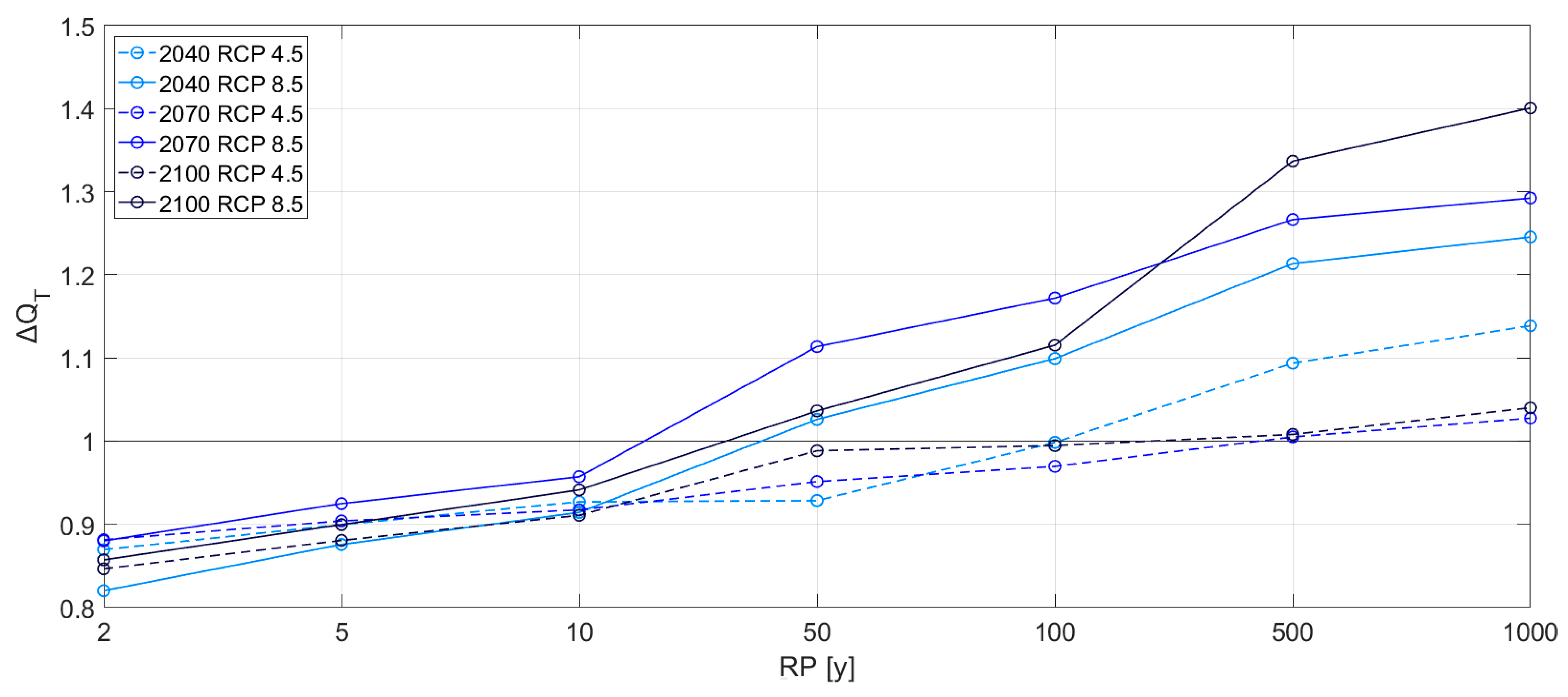
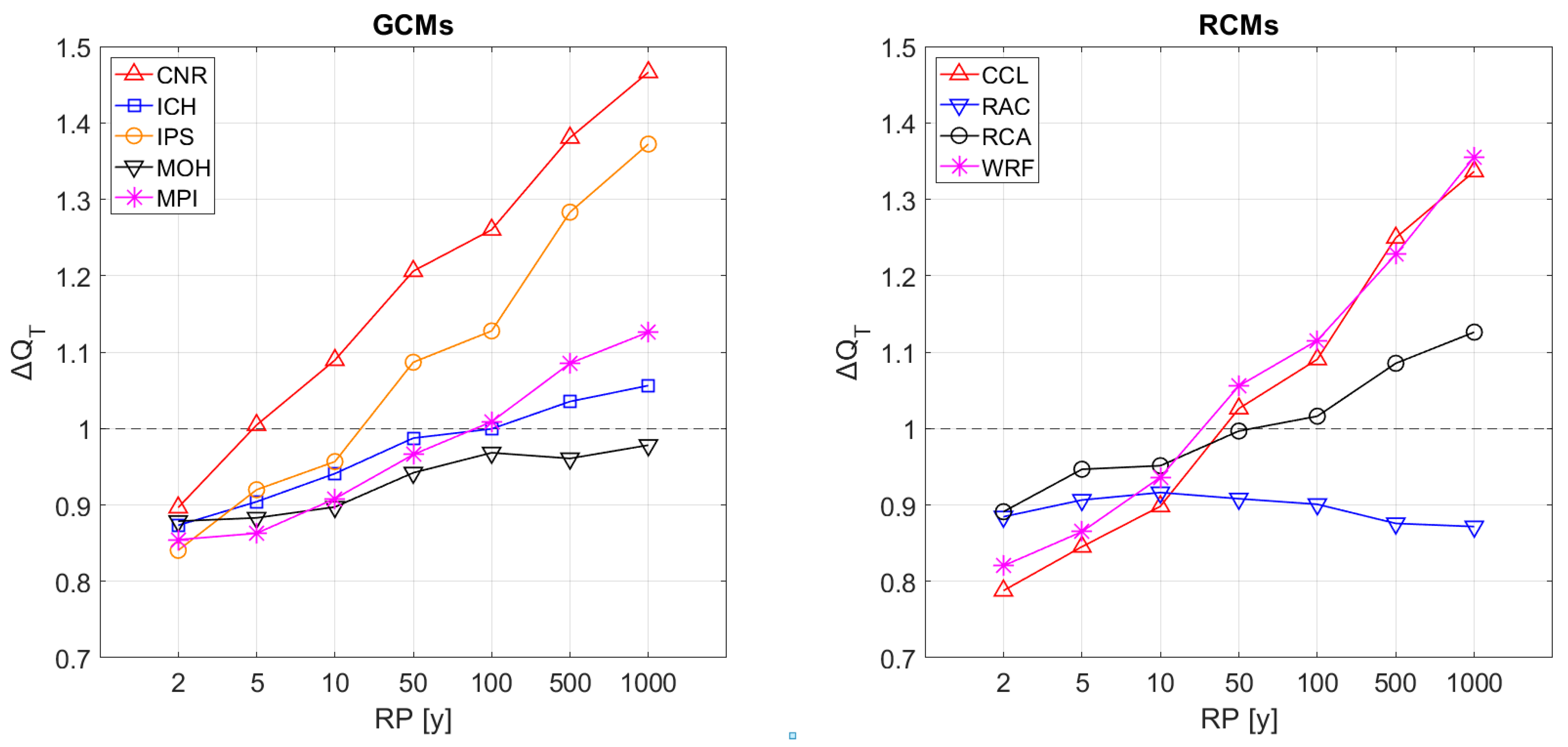
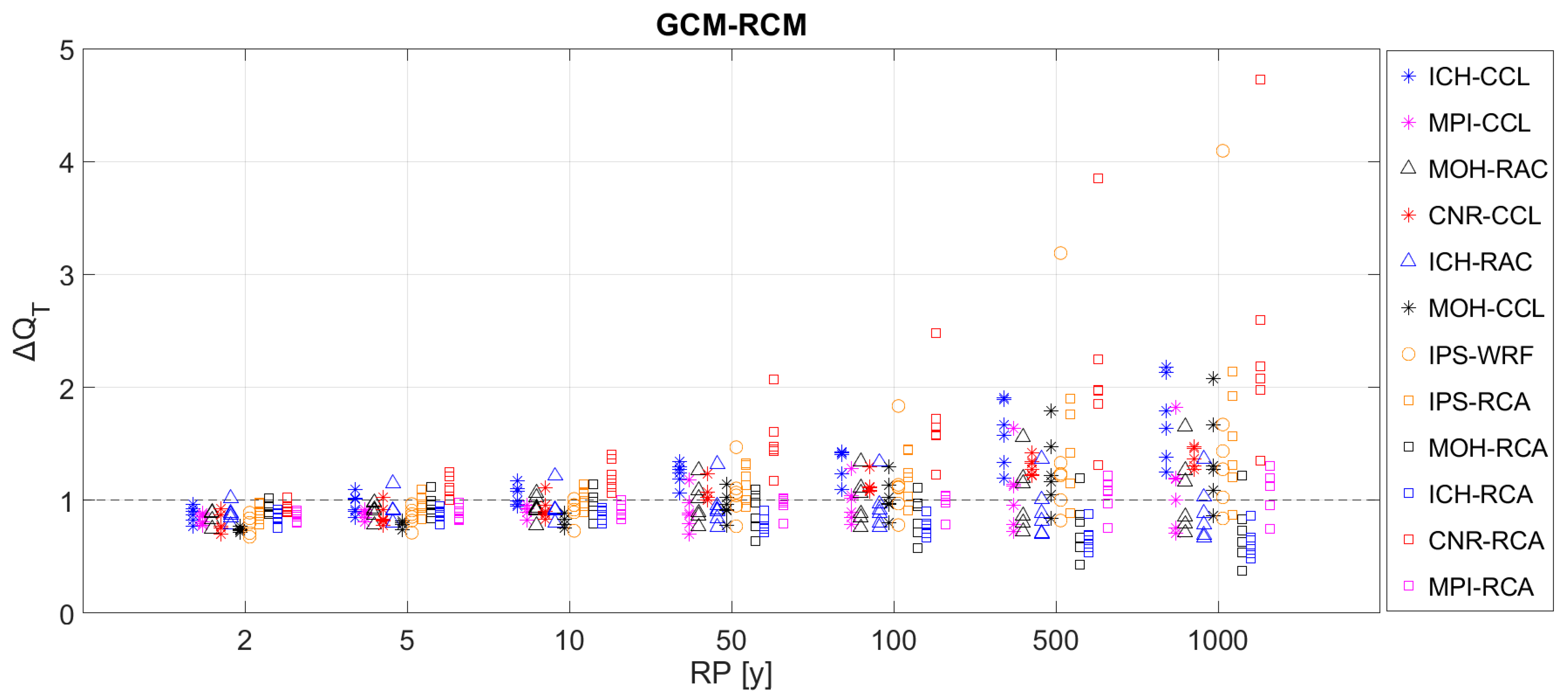
The results point to a decrease of the design peak discharges for both RCPs in the three time windows for return periods below 10 years. On the contrary, flood quantiles for return periods greater than 50 years are expected to increase for the three time windows in the RCP 8.5 scenario. In addition, the 100-year flood quantile will not change in the future if environmental policies cut greenhouse gasses emission (RCP 4.5). On the contrary, design peak discharges above 50 years are expected to increase 10–40% in the emission scenario RCP 8.5, especially for the time windows 2041–2070 and 2071–2100. GCMs seem to have more influence on the results than RCMs. The greatest increases are predicted by the results obtained with climate models that downscale from the CNRM-CM5 and IPSL-CM5A-MR GCMs.

The results of this work agree with Alfieri et al. [16] that show an increase of 100-year floods across Europe in the RCP 8.5 on average. The variation of flood quantiles in the Arga River could also be a signal for northern Spain, where a downtrend of the annual maximum flows has been found by Mediero et al. [43] and Bloesch et al. [15]. All these findings could be summarized together pointing that without a greenhouse gas emission abatement a generalized increase of the hydraulic risk for greater return periods could be expected also in the areas where the mean annual precipitation is decreasing.

Garijo and Mediero (2018) [35] found a slight decreasing trend in flood quantiles in Pamplona for RCP 4.5 and a slight increasing trend in flood quantiles for RCP 8.5 with the EURO-CORDEX climate models. In this study, clear increasing trends were obtained mainly for the RCP 8.5. The differences between both studies can be attributed to differences in the methodological approach. Garijo and Mediero (2018) used the continuous HBV model with climate projections using a daily scale, while in this study a distributed hydrological model was used with subdaily precipitations estimated with an approach based on design hyetographs and delta changes obtained from climate projections. Furthermore, the spatial distribution of the future design storms has been considered. Indeed, flood quantile delta changes have not been directly applied to the nearest rain gauges, though they have been interpolated spatially and then combined with design rainfall fields for the current scenario. This methodological approach generated 12,096 spatial distribution of rainfall for the future design storms that were used to force the RIBS hydrological model.

Comparing the results of this paper with similar studies carried out in other parts of Europe, they agree with Hennegriff et al. [30] who obtained a 15% increase in 100-year flood in Bavaria (Germany), though differing the results about the most frequent floods, as they found an increase up to 75% in the two-year floods. The results also agree with Hattermann et al. [31] who found a stronger significant increasing trend in flood frequency quantiles, reaching up to 60% increases in the 50-year floods. In addition, Sharma et al. [44] found similar increases in the most extreme floods, though analyzing climatic areas completely different from the Mediterranean area.

The most interesting result obtained in this study consist in the clear relationship between the flood hazards expected in the future the city of Pamplona and the temporal evolution of emission scenarios. Indeed, the greatest expected changes in the flood quantiles coincide with the peak of the greenhouse gasses emission in both emission scenarios: 2040 for the RCP 4.5 and in 2100 for the RCP 8.5. Therefore, results show how policies that aim to reduce greenhouse gases emissions in the future could lead to a reduction in the future flood risks. This could reduce costs related to flood damages of more extreme events and costs related to the oversized defense infrastructures.

However, the results and considerations of this study cannot be easily extrapolated to other geographical contexts. Nonetheless, they show the importance of the future hydraulic risk assessment for small and medium river basins. Indeed, small river catchments could have differing results from those obtained in large-scale studies that can only analyses the largest river basins in which they are contained.

The results also underline how important it would be to consider the increase of the future hydraulic risks due to climate change as soon as possible, especially for higher return periods and emission scenarios in which environmental policies do not aim to reduce emissions. Considering the expected increases in hydraulic risks for the 1000-year return period, decision makers could design structures such as dams avoiding spillway underestimation in the future. Similarly, the use of flood risk maps with underestimated 100-year floods could also underestimate the areas prone to flooding in urban cities.

References

1. Lal, P.N.; Mitchell, T.; Aldunce, P.; Auld, H.; Mechler, R.; Miyan, A.; Romano, L.E.; Zakaria, S.; Dlugolecki, A.; Masumoto, T.; et al. National Systems for Managing the Risks from Climate Extremes and Disasters; Cambridge University Press: Cambridge, UK; New York, NY, USA, 2012; Volume 9781107025066, ISBN 9781139177245. [Google Scholar]
2. Li, C.; Zwiers, F.; Zhang, X.; Chen, G.; Lu, J.; Li, G.; Norris, J.; Tan, Y.; Sun, Y.; Liu, M. Larger Increases in More Extreme Local Precipitation Events as Climate Warms. Geophys. Res. Lett. 2019, 46, 6885–6891. [Google Scholar] [CrossRef]
3. Donat, M.G.; Lowry, A.L.; Alexander, L.V.; O’Gorman, P.A.; Maher, N. More extreme precipitation in the world’s dry and wet regions. Nat. Clim. Chang. 2016, 6, 508–513. [Google Scholar] [CrossRef]
4. Prein, A.F.; Rasmussen, R.M.; Ikeda, K.; Liu, C.; Clark, M.P.; Holland, G.J. The future intensification of hourly precipitation extremes. Nat. Clim. Chang. 2017, 7, 48–52. [Google Scholar] [CrossRef]
5. Zhou, Q.; Leng, G.; Huang, M. Impacts of future climate change on urban flood risks: Benefits of climate mitigation and ad-aptations. Hydrol. Earth Syst. Sci. Discuss. 2016, 1–31. [Google Scholar] [CrossRef]
6. Miller, J.D.; Hutchins, M. The impacts of urbanisation and climate change on urban flooding and urban water quality: A review of the evidence concerning the United Kingdom. J. Hydrol. Reg. Stud. 2017, 12, 345–362. [Google Scholar] [CrossRef] [Green Version]
7. Tabari, H. Climate change impact on flood and extreme precipitation increases with water availability. Sci. Rep. 2020, 10, 1–10. [Google Scholar] [CrossRef]
8. Intergovernmental Panel on Climate Change IPCC. Managing the Risks of Extreme Events and Disasters to Advance Climate Change Adaptation; Cambridge University Press: Cambridge, UK, 2012. [Google Scholar] [CrossRef]
9. Hall, J.; Arheimer, B.; Borga, M.; Brázdil, R.; Claps, P.; Kiss, A.; Kjeldsen, T.R.; Kriaučiūnienė, J.; Kundzewicz, Z.W.; Lang, M.; et al. Understanding flood regime changes in Europe: A state-of-the-art assessment. Hydrol. Earth Syst. Sci. 2014, 18, 2735–2772. [Google Scholar] [CrossRef] [Green Version]
10. Quintero, F.; Mantilla, R.; Anderson, C.; Claman, D.; Krajewski, W. Assessment of changes in flood frequency due to the effects of climate change: Implications for engineering design. Hydrology 2018, 5, 19. [Google Scholar] [CrossRef] [Green Version]
11. Tofiq, F.A.; Guven, A. Prediction of design flood discharge by statistical downscaling and General Circulation Models. J. Hydrol. 2014, 517, 1145–1153. [Google Scholar] [CrossRef]
12. Pechlivanidis, I.G.; Arheimer, B.; Donnelly, C.; Hundecha, Y.; Huang, S.; Aich, V.; Samaniego, L.; Eisner, S.; Shi, P. Analysis of hydrological extremes at different hydro-climatic regimes under present and future conditions. Clim. Chang. 2017, 141, 467–481. [Google Scholar] [CrossRef] [Green Version]
13. Meinshausen, M.; Smith, S.J.; Calvin, K.; Daniel, J.S.; Kainuma, M.L.T.; Lamarque, J.; Matsumoto, K.; Montzka, S.A.; Raper, S.C.B.; Riahi, K.; et al. The RCP greenhouse gas concentrations and their extensions from 1765 to 2300. Clim. Chang. 2011, 109, 213–241. [Google Scholar] [CrossRef] [Green Version]
14. Madsen, H.; Lawrence, D.; Lang, M.; Martinkova, M.; Kjeldsen, T.R. Review of trend analysis and climate change projections of extreme precipitation and floods in Europe. J. Hydrol. 2014, 519, 3634–3650. [Google Scholar] [CrossRef] [Green Version]
15. Blöschl, G.; Hall, J.; Viglione, A.; Perdigão, R.A.P.; Parajka, J.; Merz, B.; Lun, D.; Arheimer, B.; Aronica, G.T.; Bilibashi, A.; et al. Changing climate both increases and decreases European river floods. Nature 2019, 573, 108–111. [Google Scholar] [CrossRef]
16. Alfieri, L.; Burek, P.; Feyen, L.; Forzieri, G. Global warming increases the frequency of river floods in Europe. Hydrol. Earth Syst. Sci. 2015, 19, 2247–2260. [Google Scholar] [CrossRef] [Green Version]
17. Dankers, R.; Feyen, L. Flood hazard in Europe in an ensemble of regional climate scenarios. J. Geophys. Res. Atmos. 2009, 114, 47–62. [Google Scholar] [CrossRef]
18. Rojas, R.; Feyen, L.; Bianchi, A.; Dosio, A. Assessment of future flood hazard in Europe using a large ensemble of bias-corrected regional climate simulations. J. Geophys. Res. Atmos. 2012, 117. [Google Scholar] [CrossRef]
19. Kundzewicz, Z.W.; Krysanova, V.; Dankers, R.; Hirabayashi, Y.; Kanae, S.; Hattermann, F.F.; Huang, S.; Milly, P.C.D.; Stoffel, M.; Driessen, P.P.J.; et al. Differences in flood hazard projections in Europe–their causes and consequences for decision making. Hydrol. Sci. J. 2017, 62, 1–14. [Google Scholar] [CrossRef] [Green Version]
20. Roudier, P.; Andersson, J.C.M.; Donnelly, C.; Feyen, L.; Greuell, W.; Ludwig, F. Projections of future floods and hydrological droughts in Europe under a +2 °C global warming. Clim. Chang. 2016, 135, 341–355. [Google Scholar] [CrossRef] [Green Version]
21. Hirabayashi, Y.; Mahendran, R.; Koirala, S.; Konoshima, L.; Yamazaki, D.; Watanabe, S.; Kim, H.; Kanae, S. Global flood risk under climate change. Nat. Clim. Chang. 2013, 3, 816–821. [Google Scholar] [CrossRef]
22. Herrera, S.; Fita, L.; Fernández, J.; Gutiérrez, J.M. Evaluation of the mean and extreme precipitation regimes from the ENSEMBLES regional climate multimodel simulations over Spain. J. Geophys. Res. Atmos. 2010, 115, 1–13. [Google Scholar] [CrossRef] [Green Version]
23. Pham, H.V.; Sperotto, A.; Torresan, S.; Acuña, V.; Jorda-Capdevila, D.; Rianna, G.; Marcomini, A.; Critto, A. Coupling scenarios of climate and land-use change with assessments of potential ecosystem services at the river basin scale. Ecosyst. Serv. 2019, 40, 101045. [Google Scholar] [CrossRef]
24. Zhang, Y.; You, Q.; Chen, C.; Ge, J. Impacts of climate change on streamflows under RCP scenarios: A case study in Xin River Basin, China. Atmos. Res. 2016, 178–179, 521–534. [Google Scholar] [CrossRef]
25. Stefanidis, S.; Dafis, S.; Stathis, D. Evaluation of regional climate models (RCMs) performance in simulating seasonal precipitation over Mountainous Central Pindus (Greece). Water 2020, 12, 2750. [Google Scholar] [CrossRef]
26. Giménez, P.O.; García-Galiano, S.G. Assessing Regional Climate Models (RCMs) Ensemble-driven reference evapotranspiration over Spain. Water 2018, 10, 1181. [Google Scholar] [CrossRef] [Green Version]
27. Ducharne, A.; Habets, F.; Sauquet, E.; Viennot, P.; Gascoin, S.; Hachour, A.; Martin, E.; Oudin, L.; Terray, L. Climate Change Impacts on Water Resources and Hydrological Extremes. In XVIII International Conference on Water Resources (CMWR); Carrera, J., Ed.; CIMNE: Barcelona, Spain, 2010. [Google Scholar]
28. Osuch, M.; Kindler, J.; Romanowicz, R.J.; Berbeka, K.; Banrowska, A. Adaptation Strategy of Poland to Climate Change; KLIMADA Project; Institute of Environmental Protection, National Research Institute: Warsaw, Poland, 2012. (In Polish) [Google Scholar]
29. Veijalainen, N.; Lotsari, E.; Alho, P.; Vehviläinen, B.; Käyhkö, J. National scale assessment of climate change impacts on flooding in Finland. J. Hydrol. 2010, 391, 333–350. [Google Scholar] [CrossRef]
30. Hennegriff, W.; Kolokotronis, V.; Weber, H.; Bartels, H. Climate change and floods—findings and adaptation strategies for flood protection (in German). KA Abwasser. Abfall. 2006, 53, 770–779. [Google Scholar]
31. Hattermann, F.F.; Weiland, M.; Huang, S.; Krysanova, V.; Kundzewicz, Z.W. Model-Supported Impact Assessment for the Water Sector in Central Germany under Climate Change—A Case Study. Water Resour. Manag. 2011, 25, 3113–3134. [Google Scholar] [CrossRef]
32. Garijo, C.; Mediero, L. Assessment of changes in annual maximum precipitations in the Iberian Peninsula under climate change. Water 2019, 11, 2375. [Google Scholar] [CrossRef] [Green Version]
33. Garrote, L.; Bras, R.L. A distributed model for real time forecasting using digital elevation models. J. Hydrol. 1995, 7, 279–306. [Google Scholar] [CrossRef] [Green Version]
34. Garrote, L.; Bras, R.L. An integrated software environment for real-time use of a distributed hydrologic model. J. Hydrol. 1995, 167, 307–326. [Google Scholar] [CrossRef] [Green Version]
35. Garijo, C.; Mediero, L. Influence of climate change on flood magnitude and seasonality in the Arga River catchment in Spain. Acta Geophys. 2018, 66, 769–790. [Google Scholar] [CrossRef]
36. Cabral, M.C.; Garrote, L.; Bras, R.L.; Entekhabi, D. A kinematic model of infiltration and runoff generation in layered and sloped soils. Adv. Water Resour. 1992, 15, 311–324. [Google Scholar] [CrossRef] [Green Version]
37. Mediero, L.; Garrote, L.; Martín-Carrasco, F.J. Probabilistic calibration of a distributed hydrological model for flood fore-casting. Hydrol. Sci. J. 2011, 56, 1129–1149. [Google Scholar] [CrossRef]
38. Gupta, H.V.; Sorooshian, S.; Yapo, P.O. Toward improved calibration of hydrologic models: Multiple and noncommensurable measures of information. Water Resour. Res. 1998, 34, 751–763. [Google Scholar] [CrossRef]
39. Beven, K.J. A manifesto for the equifinality thesis. J. Hydrol. 2006, 320, 18–36. [Google Scholar] [CrossRef] [Green Version]
40. Nash, J.E.; Sutcliffe, J.V. River flow forecasting through conceptual models part I—A discussion of principles. J. Hydrol. 1970, 10, 282–290. [Google Scholar] [CrossRef]
41. Luo, X.; Xu, Y.; Shi, Y. Comparison of interpolation methods for spatial precipitation under diverse orographic effects. In Proceedings of the 2011 19th International Conference on Geoinformatics, Shanghai, China, 24 June 2011. [Google Scholar] [CrossRef]
42. Jiménez-Álvarez, A.; García-Montañés, C.; Mediero, L.; Incio, L.; Garrote-Revilla, J. Bases Metodológicas del Mapa de Caudales Máximos de las Cuencas Intercomunitarias; Centro de Estudios y Experimentación de Obras Públicas: Madrid, Spain, 2014; p. 96. (In Spanish) [Google Scholar]
43. Mediero, L.; Santillán, D.; Garrote, L.; Granados, A. Detection and attribution of trends in magnitude, frequency and timing of floods in Spain. J. Hydrol. 2014, 517, 1072–1088. [Google Scholar] [CrossRef]
44. Sharma, A.; Wasko, C.; Lettenmaier, D.P. If Precipitation Extremes Are Increasing, Why Aren’t Floods? Water Resour. Res. 2018, 54, 8545–8551. [Google Scholar] [CrossRef]
Figure 1. Combination of the delta changes with the design rainfall to obtain the rainfall spatial distribution in the future.
Water 13 00792 g001
Figure 2. (a) Digital elevation model (DEM) and location of streamflow gauges. (b) Soil types and location of rain gauges.
Water 13 00792 g002
Figure 3. Floods selected in the A323 hydrometer by using a peak-over-threshold (POT) analysis with a threshold of 300 m3/s.
Water 13 00792 g003
Figure 4. Objective function results for the five flood events considered in the calibration process. Columns show flood events. Rows show the relationship between each objective function and Nash–Sutcliffe efficiency coefficient (NSE). Red circles represent the combination of parameter values selected for the validation procedure.
Water 13 00792 g004
Figure 5. NSE objective function results for the five flood events considered in the calibration process. Columns show flood events. Rows show the three parameters used to calibrate the model: f, K v , C v . Red circles represent the combination of best combination of parameter values identified in the calibration process.
Water 13 00792 g005
Figure 6. Comparison between observed (black) and simulated (red) hydrographs for the calibration and validation flood events with the parameter values selected in the calibration process. Columns show flood events. Rows show streamflow gauging-sites.
Water 13 00792 g006
Figure 7. Hydrographs for the current (dashed black) and climate change (colored) scenarios for the CNR-CCL climate model in the three periods. Columns show return periods. The upper row shows results for the representative concentration pathways RCP 4.5 and the lower row for the RCP 8.5.
Water 13 00792 g007
Figure 8. Boxplots of ΔQT values for the 12 climate models considered in the study. The upper row shows the results for the RCP 4.5 and the lower row for the RCP 8.5. The first column shows the results for the 2011–2040 period, the second for the 2041–2070 period, and the third for the 2071–2100 period.
Water 13 00792 g008
Figure 9. Median values of expected flood changes in the three time windows and two emission scenarios.
Water 13 00792 g009
Figure 10. Median values of ΔQT for the three periods in the future and two RCPs. The results are shown for each return period grouped by global climate models (GCMs) (left) and regional climate models (RCMs) (right).
Water 13 00792 g010
Figure 11. Median values of ΔQT for each combination of GCM and RCM.
Water 13 00792 g011