
Water Demand Prediction Using Machine Learning Methods: A Case Study of the Beijing–Tianjin–Hebei Region in China


Abstract
1. Introduction
2. Literature Review
2.1. Variables Considered in the Literature for Explaining Water Demand

| Explanatory variables | Unit | Lu et al. [11] | Li et al. [12] | Zhao and Chen [13] | Tian and Xue [14] | Zhang et al. [15] | Sun et al. [16] | Tang et al. [17] | Zhang et al. [18] | Wang et al. [19] | Tiwari et al. [20] | Chen et al. [21] | |
|---|---|---|---|---|---|---|---|---|---|---|---|---|---|
| Economy | GDP | Billion Yuan | √ | √ | √ | √ | √ | √ | |||||
| Per capita GDP | Yuan per Person | √ | √ | √ | |||||||||
| Added value of primary industry | Billion Yuan | √ | √ | √ | √ | ||||||||
| Added value of secondary industry | Billion Yuan | √ | √ | ||||||||||
| Added value of tertiary industry | Billion Yuan | √ | √ | √ | |||||||||
| Per capita disposable income | Yuan | √ | √ | √ | |||||||||
| Community | Year-end population | Million | √ | √ | √ | √ | √ | √ | √ | ||||
| Water use | Agricultural water consumption | Billion m3 | √ | √ | √ | ||||||||
| Irrigated area | Thousand Hectare | √ | √ | √ | √ | ||||||||
| Resource availability | Total water resources | Billion m3 | √ | ||||||||||
| Annual precipitation | mm | √ | √ | √ | |||||||||
2.2. Models for Predicting Water Demand
3. Methodology
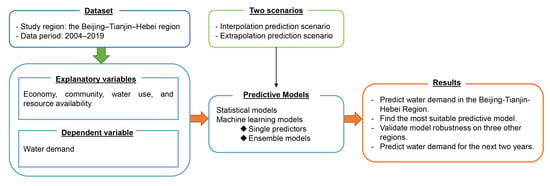
3.1. Research Design
- (1)
- Interpolation prediction scenario (IPS): For each model, a 10-fold CV was applied to randomly selected training samples accounting for 80% of all the data. The fitted models were then tested on the remaining 20% of the data to verify their prediction performance.
- (2)
- Extrapolation prediction scenario (EPS): For each model, a 10-fold CV was applied to the training data covering the period from 2004 to 2018. The fitted models were then tested on the 2019 data.
3.2. Data Preprocessing
3.3. Modeling
- Statistical models: linear regression (LR), ridge regression, least absolute shrinkage and selection operator (lasso) regression, kernel ridge regression (KRR), and Bayesian ridge regression (BRR);
- Machine learning models:
- ➢
- Single predictors: backpropagation neural network (BPNN), decision tree (DT), and support vector machine (SVM);
- ➢
- Ensemble methods: random forest (RF), adaptive boosting (AdaBoost), and gradient-boosting decision tree (GBDT). RF is a parallel integration algorithm, whereas AdaBoost and GBDT are serial-integration algorithms.
3.3.1. Linear Regression
3.3.2. Ridge and Lasso Regression
3.3.3. Kernel and Bayesian Ridge Regression
3.3.4. Backpropagation Neural Network
3.3.5. Decision Tree
3.3.6. Support Vector Machine
3.3.7. Random Forest
3.3.8. AdaBoost
3.3.9. Gradient Boosting Decision Tree
3.4. Model Training
3.5. Cross-Validation
3.6. Model Testing
4. Cast Study: Beijing–Tianjin–Hebei Region in China
4.1. Study Region
4.2. Dataset
- Economy: GDP, per capita GDP, added value of primary industry, added value of secondary industry, added value of tertiary industry, and per capita disposable income;
- Community: year-end population;
- Water use: agriculture water consumption and irrigated area;
- Resource availability: total water resources and annual precipitation.
4.3. Predictive Results
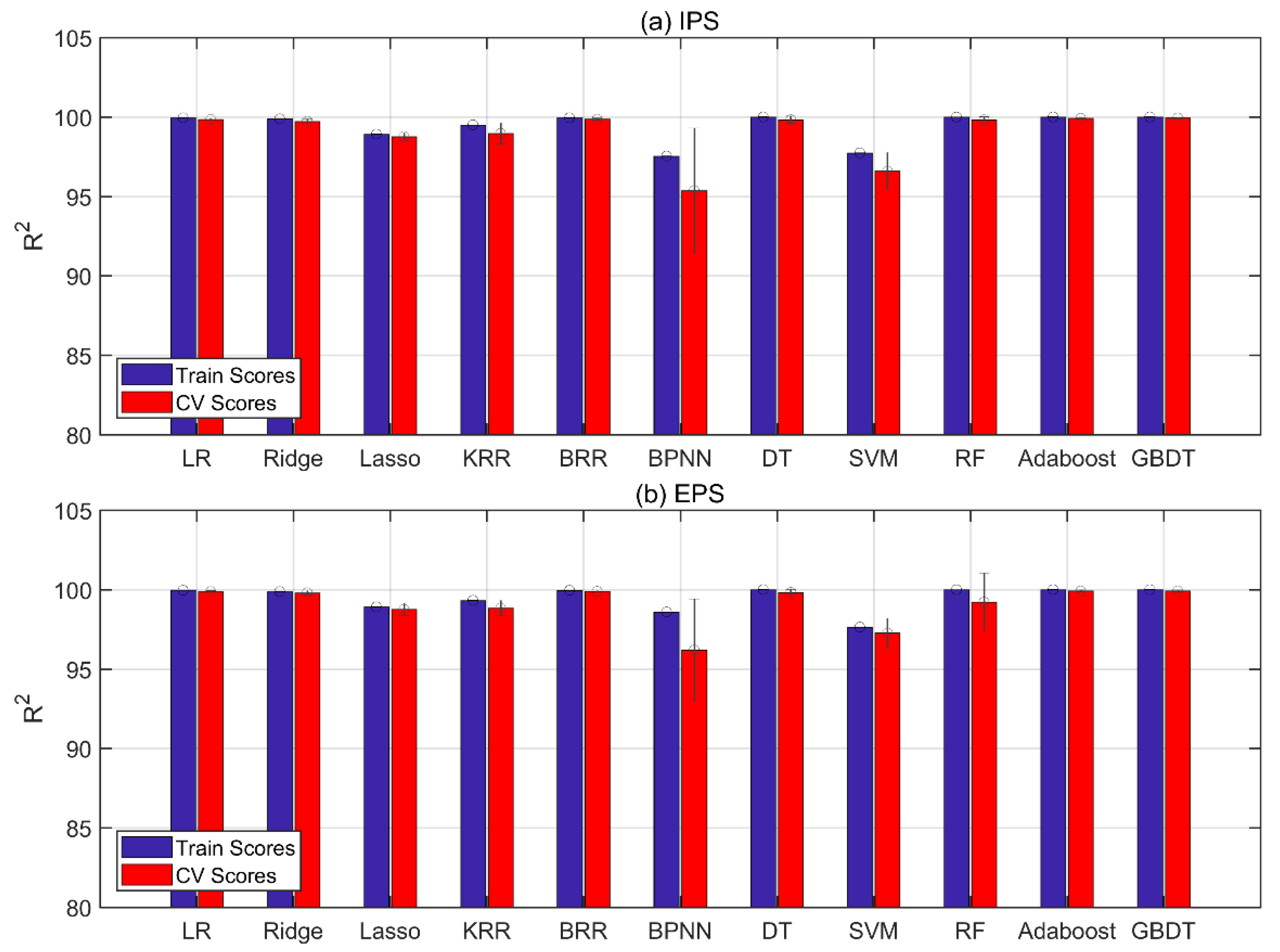
4.3.1. Training and CV Results
4.3.2. Test Results
4.3.3. Model Robustness
4.3.4. Prediction for the Next Two Years
5. Conclusions
Author Contributions
Funding
Institutional Review Board Statement
Informed Consent Statement
Data Availability Statement
Conflicts of Interest
Appendix A
| Variables | Units | Mean | Std | Min | Max |
|---|---|---|---|---|---|
| Water demand | Billion m3 | 8.45 | 7.74 | 2.21 | 20.4 |
| GDP | Billion Yuan | 1736.35 | 936.79 | 311.10 | 3537.13 |
| Per capita GDP | Yuan per Person | 66,566.60 | 37,324.61 | 12,487.00 | 16,422.00 |
| Added value of primary industry | Billion Yuan | 98.21 | 129.20 | 8.74 | 351.84 |
| Added value of secondary industry | Billion Yuan | 671.37 | 422.17 | 168.60 | 1584.62 |
| Added value of tertiary industry | Billion Yuan | 966.78 | 655.00 | 131.98 | 2954.25 |
| Per capita disposable income | Yuan | 28,810.09 | 15,283.60 | 7951.31 | 73,848.51 |
| Year-end population | Million | 35.02 | 26.79 | 10.24 | 75.92 |
| Agricultural water consumption | Billion m3 | 5.38 | 6.20 | 0.37 | 15.69 |
| Irrigated area | Thousand Hectare | 1668.90 | 2030.30 | 109.24 | 4603.07 |
| Total water resources | Billion m3 | 6.37 | 6.48 | 0.81 | 23.55 |
| Annual precipitation | mm | 531.89 | 85.15 | 408.20 | 850.30 |
References
- Greve, P.; Kahil, T.; Mochizuki, J.; Schinko, T.; Satoh, Y.; Burek, P.; Fischer, G.; Tramberend, S.; Burtscher, R.; Langan, S.; et al. Global assessment of water challenges under uncertainty in water scarcity projections. Nat. Sustain. 2018, 1, 486–494. [Google Scholar] [CrossRef]
- Bakkes, J.A.; Bosch, P.R.; Bouwman, A.F.; Eerens, H.C.; Den Elzen, M.; Isaac, M.; Janssen, P.; Goldewijk, K.K.; Kram, T.; De Leeuw, F.; et al. (Eds.) Background Report to the OECD Environmental Outlook to 2030: Overviews, Details, and Methodology of Model-Based Analysis; Netherlands Environmental Assessment Agency (MNP): Bilthoven, The Netherlands, 2008. [Google Scholar]
- House-Peters, L.A.; Chang, H. Urban water demand modeling: Review of concepts, methods, and organizing principles. Water Resour. Res. 2011, 47, 5. [Google Scholar] [CrossRef]
- Pacchin, E.; Gagliardi, F.; Alvisi, S.; Franchini, M. A Comparison of Short-Term Water Demand Forecasting Models. Water Resour. Manag. 2019, 33, 1481–1497. [Google Scholar] [CrossRef]
- Pesantez, J.; Berglund, E.Z.; Kaza, N. Smart meters data for modeling and forecasting water demand at the user-level. Environ. Model. Softw. 2020, 125, 104633. [Google Scholar] [CrossRef]
- Derrible, S. Urban infrastructure is not a tree: Integrating and decentralizing urban infrastructure systems. Environ. Plan. B Urban Anal. City Sci. 2017, 44, 553–569. [Google Scholar] [CrossRef]
- Beijing Water Authority. Water Resources Reports for Beijing. 2019. Available online: http://swj.beijing.gov.cn/ (accessed on 10 November 2020).
- Tianjin Water Authority. Water Resources Reports for Tianjin. 2019. Available online: http://swj.tj.gov.cn/ (accessed on 10 November 2020).
- Department of Water Resources of Hebei Province. Water Resources Reports of Hebei Province. 2019. Available online: http://slt.hebei.gov.cn/ (accessed on 10 November 2020).
- China Statistics Bureau. China Statistics Yearbook. Beijing: China Statistics Bureau. 2019. Available online: http://www.stats.gov.cn/ (accessed on 10 November 2020).
- Lu, H.; Matthews, J.; Han, S. A hybrid model for monthly water demand prediction: A case study of Austin, Texas. AWWA Water Sci. 2020, 2, 1175. [Google Scholar] [CrossRef]
- Li, M.; Finlayson, B.; Webber, M.; Barnett, J.; Webber, S.; Rogers, S.; Chen, Z.; Wei, T.; Chen, J.; Wu, X.; et al. Estimating urban water demand under conditions of rapid growth: The case of Shanghai. Reg. Environ. Chang. 2017, 17, 1153–1161. [Google Scholar] [CrossRef]
- Zhao, Y.; Chen, X.J. Prediction Model on Urban Residential Water Based on Resilient BP Learning Algorithm. Appl. Mech. Mater. 2014, 543, 4086–4089. [Google Scholar] [CrossRef]
- Tian, T.; Xue, H. Prediction of annual water consumption in Guangdong Province based on Bayesian neural network. IOP Conf. Series Earth Environ. Sci. 2017, 69, 12032. [Google Scholar] [CrossRef]
- Zhang, Z.G.; Shao, Y.S.; Xu, Z.X. Prediction of urban water demand on the basis of Engel’s coefficient and Hoffmann index: Case studies in Beijing and Jinan, China. Water Sci. Technol. 2010, 62, 410–418. [Google Scholar]
- Sun, Y.; Liu, N.; Shang, J.; Zhang, J. Sustainable utilization of water resources in China: A system dynamics model. J. Clean. Prod. 2017, 142, 613–625. [Google Scholar] [CrossRef]
- Tang, Z.Q.; Liu, G.; Xu, W.N.; Xia, Z.Y.; Xiao, H. Water Demand Forecasting in Hubei Province with BP Neural Network Model. Adv. Mater. Res. 2012, 599, 701–704. [Google Scholar] [CrossRef]
- Zhang, Q.; Diao, Y.; Dong, J. Regional Water Demand Prediction and Analysis Based on Cobb-Douglas Model. Water Resour. Manag. 2013, 27, 3103–3113. [Google Scholar] [CrossRef]
- Wang, H.; Wang, W.; Cui, Z.; Zhou, X.; Zhao, J.; Ya, L. A new dynamic firefly algorithm for demand estimation of water resources. Inf. Sci. 2018, 438, 95–106. [Google Scholar] [CrossRef]
- Tiwari, M.K.; Adamowski, J.F. Medium-Term Urban Water Demand Forecasting with Limited Data Using an Ensemble Wavelet–Bootstrap Machine-Learning Approach. J. Water Resour. Plan. Manag. 2015, 141, 04014053. [Google Scholar] [CrossRef]
- Chen, X.; Li, F.; Li, X.; Hu, Y.; Hu, P. Evaluating and mapping water supply and demand for sustainable urban ecosystem management in Shenzhen, China. J. Clean. Prod. 2020, 251, 119754. [Google Scholar] [CrossRef]
- Fricke, K. Analysis and Modelling of Water Supply and Demand under Climate Change, Land Use Transformation and Socio-Economic Development: The Water Resource Challenge and Adaptation Measures for Urumqi Region, Northwest China; Springer Science & Business Media: Berlin, Germany, 2013. [Google Scholar]
- Donkor, E.A.; Mazzuchi, T.A.; Soyer, R.; Roberson, J.A. Urban Water Demand Forecasting: Review of Methods and Models. J. Water Resour. Plan. Manag. 2014, 140, 146–159. [Google Scholar] [CrossRef]
- Mitchell, T.M. Machine Learning; McGraw-Hill Education: New York, NY, USA, 1997. [Google Scholar]
- Arbues, F.; Villanua, I. Potential for Pricing Policies in Water Resource Management: Estimation of Urban Residential Water Demand in Zaragoza, Spain. Urban Stud. 2006, 43, 2421–2442. [Google Scholar] [CrossRef]
- House-Peters, L.; Pratt, B.; Chang, H. Effects of Urban Spatial Structure, Sociodemographics, and Climate on Residential Water Consumption in Hillsboro, Oregon1. JAWRA J. Am. Water Resour. Assoc. 2010, 46, 461–472. [Google Scholar] [CrossRef]
- Kontokosta, C.E.; Jain, R.K. Modeling the determinants of large-scale building water use: Implications for data-driven urban sustainability policy. Sustain. Cities Soc. 2015, 18, 44–55. [Google Scholar] [CrossRef]
- Ashoori, N.; Dzombak, D.A.; Small, M.J. Modeling the Effects of Conservation, Demographics, Price, and Climate on Urban Water Demand in Los Angeles, California. Water Resour. Manag. 2016, 30, 5247–5262. [Google Scholar] [CrossRef]
- Hastie, T.; Tibshirani, R.; Friedman, J. The Elements of Statistical Learning; Springer: Berlin, Germany, 2009; pp. 43–99. [Google Scholar]
- Lee, D.; Derrible, S. Predicting Residential Water Demand with Machine-Based Statistical Learning. J. Water Resour. Plan. Manag. 2020, 146, 04019067. [Google Scholar] [CrossRef]
- Mu, L.; Zheng, F.; Tao, R.; Zhang, Q.; Kapelan, Z. Hourly and Daily Urban Water Demand Predictions Using a Long Short-Term Memory Based Model. J. Water Resour. Plan. Manag. 2020, 146, 05020017. [Google Scholar] [CrossRef]
- Villarin, M.C.; Rodriguez-Galiano, V.F. Machine Learning for Modeling Water Demand. J. Water Resour. Plan. Manag. 2019, 145, 04019017. [Google Scholar] [CrossRef]
- Rozos, E.; Butler, D.; Makropoulos, C. An integrated system dynamics–cellular automata model for distributed water-infrastructure planning. Water Sci. Tech. Water Supply 2016, 16, 1519–1527. [Google Scholar] [CrossRef]
- Golshani, N.; Shabanpour, R.; Mahmoudifard, S.M.; Derrible, S.; Mohammadian, A. Modeling travel mode and timing decisions: Comparison of artificial neural networks and copula-based joint model. Travel Behav. Soc. 2018, 10, 21–32. [Google Scholar] [CrossRef]
- Lee, D.; Derrible, S.; Pereira, F.C. Comparison of Four Types of Artificial Neural Network and a Multinomial Logit Model for Travel Mode Choice Modeling. Transp. Res. Rec. J. Transp. Res. Board 2018, 2672, 101–112. [Google Scholar] [CrossRef]
- Ali, S.; Wu, K.; Weston, K.; Marinakis, D. A Machine Learning Approach to Meter Placement for Power Quality Estimation in Smart Grid. IEEE Trans. Smart Grid 2015, 7, 1552–1561. [Google Scholar] [CrossRef]
- Marvuglia, A.; Messineo, A. Monitoring of wind farms’ power curves using machine learning techniques. Appl. Energy 2012, 98, 574–583. [Google Scholar] [CrossRef]
- García, V.; Marqués, A.; Sánchez-Garreta, J. Exploring the synergetic effects of sample types on the performance of ensembles for credit risk and corporate bankruptcy prediction. Inf. Fusion 2019, 47, 88–101. [Google Scholar] [CrossRef]
- Xia, Y.; Liu, C.; Li, Y.; Liu, N. A boosted decision tree approach using Bayesian hyper-parameter optimization for credit scoring. Expert Syst. Appl. 2017, 78, 225–241. [Google Scholar] [CrossRef]
- Voyant, C.; Notton, G.; Kalogirou, S.; Nivet, M.; Paoli, C.; Motte, F.; Fouilloy, A. Machine learning methods for solar radiation forecasting: A review. Renew. Energy 2017, 105, 569–582. [Google Scholar] [CrossRef]
- Muñoz-Mas, R.; Gil-Martínez, E.; Oliva-Paterna, F.J.; Belda, E.J. and Martínez-Capel, F. Tree-based ensembles unveil the microhabitat suitability for the invasive bleak (Alburnus alburnus L.) and pumpkinseed (Lepomis gibbosus L.): Introducing XGBoost to eco-informatics. Ecol. Inform. 2019, 53. [Google Scholar] [CrossRef]
- Darling, E.S.; Alvarez-Filip, L.; Oliver, T.A.; McClanahan, T.R.; Côté, I.M. Evaluating life-history strategies of reef corals from species traits. Ecol. Lett. 2012, 15, 1378–1386. [Google Scholar] [CrossRef]
- Archibald, S.; Roy, D.P.; Van Wilgen, B.W.; Scholes, R.J. What limits fire? An examination of drivers of burnt area in Southern Africa. Glob. Chang. Biol. 2009, 15, 613–630. [Google Scholar] [CrossRef]
- Rozos, E. Machine Learning, Urban Water Resources Management and Operating Policy. Resources 2019, 8, 173. [Google Scholar] [CrossRef]
- Nascimento, D.S.; Coelho, A.L.; Canuto, A.M. Integrating complementary techniques for promoting diversity in classifier ensembles: A systematic study. Neurocomputing 2014, 138, 347–357. [Google Scholar] [CrossRef]
- Lessmann, S.; Baesens, B.; Seow, H.-V.; Thomas, L.C. Benchmarking state-of-the-art classification algorithms for credit scoring: An update of research. Eur. J. Oper. Res. 2015, 247, 124–136. [Google Scholar] [CrossRef]
- Parisouj, P.; Mohebzadeh, H.; Lee, T. Employing Machine Learning Algorithms for Streamflow Prediction: A Case Study of Four River Basins with Different Climatic Zones in the United States. Water Resour. Manag. 2020, 34, 4113–4131. [Google Scholar] [CrossRef]
- Sengupta, A.; Hawley, R.J.; Stein, E.D. Predicting Hydromodification in Streams Using Nonlinear Memory-Based Algorithms in Southern California Streams. J. Water Res. Plan. Mang. 2018, 144, 144. [Google Scholar] [CrossRef]
- Pedregosa, F.; Varoquaux, G.; Gramfort, A.; Michel, V.; Thirion, B.; Grisel, O.; Blondel, M.; Prettenhofer, P.; Weiss, R.; Dubourg, V.; et al. Scikit-learn: Machine learning in Python. J. Mach. Learn. Res. 2011, 12, 2825–2830. [Google Scholar]
- API Design for Machine Learning Software: Experiences from the Scikit-Learn Project. Available online: https://arxiv.org/pdf/1309.0238.pdf (accessed on 1 July 2020).
- Hoerl, A.E.; Kennard, R.W. Ridge regression: Applications to nonorthogonal problems. Technometrics. 1970, 12, 69–82. [Google Scholar] [CrossRef]
- Khan, M.H.R.; Bhadra, A.; Howlader, T. Stability selection for lasso, ridge and elastic net implemented with AFT models. Stat Appl. Genet Mol. 2019, 18. [Google Scholar] [CrossRef] [PubMed]
- Tibshirani, R. Regression shrinkage and selection via the lasso. J. R. Stat. Soc. Ser. B 1996, 58, 267–288. [Google Scholar] [CrossRef]
- Geng, S.; Wang, X. Research on data-driven method for circuit breaker condition assessment based on back propagation neural network. Comput. Electr. Eng. 2020, 86, 106732. [Google Scholar] [CrossRef]
- Cortes, C.; Vapnik, V. Support-vector networks. Mach. Learn. 1995, 20, 273–297. [Google Scholar] [CrossRef]
- Breiman, L. Random forests. Mach. Learn. 2001, 45, 5–32. [Google Scholar] [CrossRef]
- Freund, Y.; Schapire, R.E. Experiments with a new boosting algorithm. In Machine Learning: Proceedings of the Thirteenth International Conference; Saitta, L., Ed.; Morgan Kaufmann Publishers: San Francisco, CA, USA, 1996. [Google Scholar]
- Feng, D.-C.; Liu, Z.-T.; Wang, X.-D.; Jiang, Z.-M.; Liang, S.-X. Failure mode classification and bearing capacity prediction for reinforced concrete columns based on ensemble machine learning algorithm. Adv. Eng. Inform. 2020, 45, 101126. [Google Scholar] [CrossRef]
- Friedman, J.H. Greedy function approximation: A gradient boosting machine. Ann. Stat. 2001, 1189–1232. [Google Scholar] [CrossRef]
- Ebrahimi, M.; Mohammadi-Dehcheshmeh, M.; Ebrahimie, E.; Petrovski, K. Comprehensive analysis of machine learning models for prediction of sub-clinical mastitis: Deep Learning and Gradient-Boosted Trees outperform other models. Comput. Biol. Med. 2019, 114, 103456. [Google Scholar] [CrossRef]
- Zhao, D.; Tang, Y.; Liu, J.; Tillotson, M.R. Water footprint of Jing-Jin-Ji urban agglomeration in China. J. Clean. Prod. 2017, 167, 919–928. [Google Scholar] [CrossRef]
- Zhang, Z.; Shi, M.; Yang, H. Understanding Beijing’s Water Challenge: A Decomposition Analysis of Changes in Beijing’s Water Footprint between 1997 and 2007. Environ. Sci. Technol. 2012, 46, 12373–12380. [Google Scholar] [CrossRef] [PubMed]
- Derrible, S. An approach to designing sustainable urban infrastructure. MRS Energy Sustain. 2019, 5, 5. [Google Scholar] [CrossRef]
- Sichuan Provincal Water Resources Department. Water Resources Reports for Sichuan. 2019. Available online: http://slt.sc.gov.cn/scsslt/xzfw/szy_list.shtml (accessed on 10 November 2020).
- Chongqing Water Resources Department. Water Resources Reports for Chongqing. 2019. Available online: http://slj.cq.gov.cn/zwgk_250/fdzdgknr/tjgb/ (accessed on 10 November 2020).
- HeiLongJiang Provincal Water Resources Department. Water Resources Reports for HeiLongJiang Province. 2019. Available online: http://slt.hlj.gov.cn/channels/154.html (accessed on 10 November 2020).
- Jilin Provincal Water Resources Department. Water Resources Reports for Jilin. 2019. Available online: http://slt.jl.gov.cn/zwgk/szygb/ (accessed on 10 November 2020).
- Henan Provincal Water Resources Department. Water Resources Reports for Henan. 2019. Available online: http://slt.henan.gov.cn/bmzl/szygl/szygb/ (accessed on 10 November 2020).
- Shanxi Provincal Department of Water Resources. Water Resources Reports for Shanxi. 2019. Available online: http://slt.shanxi.gov.cn/zncs/szyc/szygb/ (accessed on 10 November 2020).
- Anhui Water Resources Department. Water Resources Reports for Anhui. 2019. Available online: http://slt.ah.gov.cn/tsdw/swj/szyshjjcypj/ (accessed on 10 November 2020).
- Water Resources Department of Shandong Province. Water Resources Reports for Shandong. 2019. Available online: http://wr.shandong.gov.cn/ (accessed on 10 November 2020).
- Moriasi, D.N.; Arnold, J.G.; Van Liew, M.W.; Bingner, R.L.; Harmel, R.D.; Veith, T.L. Model Evaluation Guidelines for Systematic Quantification of Accuracy in Watershed Simulations. Trans. ASABE 2007, 50, 885–900. [Google Scholar] [CrossRef]
- Miraji, M.; Liu, J.; Zheng, C. The impacts of water demand and its implications for future surface water resource management: The case of tanzania’s wami ruvu basin (WRB). Water 2019, 11, 1280. [Google Scholar] [CrossRef]
- The People’s Government of Sichuan Province. 2012 Sichuan Province Work Report. 2012. Available online: http://www.gov.cn/test/2012-02/02/content_2056707.htm (accessed on 20 January 2021).
- Li, T. Binhai New Area of Tianjin Development Report; Annual Report on the Development of China’s Special Economic Zones(2018); Social Science Academic Press: Beijing, China, 2019. [Google Scholar]


| IPS | ||||
|---|---|---|---|---|
| Metric | LR | BRR | AdaBoost | GBDT |
| MSE | 0.00010812 | 0.00010758 | 0.00000057 | 0.00000016 |
| MAE | 0.00906555 | 0.00929241 | 0.00040798 | 0.00032787 |
| R2 (%) | 99.9468% | 99.9470% | 99.9997% | 99.9999% |
| EPS | ||||
| Metric | LR | BRR | AdaBoost | GBDT |
| MSE | 0.00079666 | 0.00053748 | 0.00009235 | 0.00006178 |
| MAE | 0.02147535 | 0.01805283 | 0.00720000 | 0.00584230 |
| R2 (%) | 99.4558% | 99.6329% | 99.9369% | 99.9578% |
Publisher’s Note: MDPI stays neutral with regard to jurisdictional claims in published maps and institutional affiliations. |
© 2021 by the authors. Licensee MDPI, Basel, Switzerland. This article is an open access article distributed under the terms and conditions of the Creative Commons Attribution (CC BY) license (http://creativecommons.org/licenses/by/4.0/).
Share and Cite
Shuang, Q.; Zhao, R.T. Water Demand Prediction Using Machine Learning Methods: A Case Study of the Beijing–Tianjin–Hebei Region in China. Water 2021, 13, 310. https://doi.org/10.3390/w13030310
Shuang Q, Zhao RT. Water Demand Prediction Using Machine Learning Methods: A Case Study of the Beijing–Tianjin–Hebei Region in China. Water. 2021; 13(3):310. https://doi.org/10.3390/w13030310
Chicago/Turabian StyleShuang, Qing, and Rui Ting Zhao. 2021. "Water Demand Prediction Using Machine Learning Methods: A Case Study of the Beijing–Tianjin–Hebei Region in China" Water 13, no. 3: 310. https://doi.org/10.3390/w13030310
APA StyleShuang, Q., & Zhao, R. T. (2021). Water Demand Prediction Using Machine Learning Methods: A Case Study of the Beijing–Tianjin–Hebei Region in China. Water, 13(3), 310. https://doi.org/10.3390/w13030310