Discharge Estimation with the Use of Unmanned Aerial Vehicles (UAVs) and Hydraulic Methods in Shallow Rivers

Abstract

Although river discharge is essential hydrologic information, it is often absent, especially for small rivers and remote catchment areas. Practical difficulties frequently impede the installation and operation of gauging stations, while satellite-sensed data have proved to be relatively useful only for discharge estimation of large-scale rivers. In this study, we propose a new methodology based on UAV-sensed data and photogrammetry techniques combined with empirical hydraulic equations for discharge estimation. In addition, two different riverbed particle size distributions were incorporated, to study the effect of fine sediment inclusion (or exclusion) in the estimation process. Accordingly, 17 study sites were selected and six different approaches were applied in each. Results show that at 75% of sites at least one approach produced an accurate discharge estimation, while in 10 out the 17 sites (58.8%) all six approaches produced accurate estimations. A strong correlation between a threshold value for the hydraulic radius (Rh = 0.3 m) of cross-sections and high estimation errors for sites exceeding it was also observed. The fine sediment inclusion improved only the performance of certain approaches and did not have a consistently positive effect. Overall, the relatively high percentage of sites with satisfactory discharge estimates indicates that using UAV-derived data and simple hydraulic equations can be used for this purpose, with an acceptable level of accuracy.

1. Introduction

River discharge is one of the most important variables in hydrology and constitutes fundamental information [1,2] in the fields of environmental monitoring and in water management operations. However, measurements of discharge are often absent as conventional gauging methods are expensive and impractical as well as hard to deploy and maintain [3,4]. These limitations are particularly true for water bodies located in remote locations, for rivers and streams with ephemeral flow and for small catchment areas. This is of great concern, since the latter are impacted from flash floods, one of the most significant natural hazards, known to cause serious loss of life and economic damage [5], especially in Mediterranean regions [6].

In the last decades, remote sensing has been extensively used as a source of primary data in environmental studies, as it can overcome the aforementioned limitations. Encompassing a wide range of temporal and spatial extents, remotely sensed data can be the product of satellite missions [7], airborne laser scanning [8], multibeam echo sounding methods [9], terrestrial laser scanning [10] and finally UAVs. Remote sensing of river discharge has been the scope of numerous scientific studies and experimental setups, but until now, no remote sensing platform has the ability to directly measure river discharge [11]. As a result, discharge is usually estimated via proxies, including remote sensing observations of water surface elevation, river width and water surface slope [12], combined with some discharge equation. The Manning equation has been noted to produce positive results on discharge estimation in numerous studies with quite diverse data sources, from satellite [13,14] to UAVs [15,16]. The outcomes of such studies suggest that the Manning equation is a rather credible solution for similar research projects. In the last two decades, many studies have experimented in the field of river discharge estimation from satellite data [17,18,19,20]. Yet, satellite remote sensing platforms have serious limitations on temporal and spatial scales, making this approach unsuitable for medium and small scale rivers (narrower than 100 m) [21]; the low spatial resolution data lead to critical scale discrepancy between data sources and the models used [22], while the lack of control on the revisiting period of the sensor over the selected site [23] is another significant constraint. Moreover, the overall operation and data delivery of satellite platforms are under the auspices of large organizations or agencies [24].

The demand for fine scale remote sensing has led to the introduction of Unmanned Aerial Vehicles (UAVs), which have proven to be efficient in a vast range of applications in environmental monitoring and management [25]. Given the advantages of low cost, ease of use, full operational control to the user and high-resolution spatial data, low-altitude UAVs have been filling the gap between satellite-born data and ground monitoring. As a result, UAVs are increasingly being used in new studies, covering a wide range of different methodologies and adapted sensors.

Detert et al. [26] recently demonstrated the use of low-cost UAVs for the estimation of river flow measurements. In that research, the recorded airborne video was used to determine flow velocities and surface flow fields via particle image velocimetry (PIV) and river bathymetry through the application of photogrammetry methods. Similarly, using large-scale particle image velocimetry (LSPIV) on video captures from UAV, Lewis et al. [27] managed, through a basic setup, to produce accurate estimates of discharge over ten streams and small rivers in East-Central Illinois, USA. In an innovative study, Zhao et al. [28] proposed a new framework for estimation of streamflow in medium-to-small rivers where ground measurements are limited, with the pairing of high-resolution UAV imagery and the introduction of a new virtual hydraulic radius (VHR) method to provide the initial values of the AMHG (at-many-stations hydraulic geometry) parameters. Dealing with non-uniform flow modelling, Kang et al. [29] estimated streamflow with the aid of optical, infrared and microwave sensors on a UAV.

Using a different set-up, Kinzel and Legleiter [30] proposed a combination of a thermal infrared camera and a PIV algorithm to approximate surface flow velocity combined with a polarizing LiDAR for bathymetry measurement, in order to estimate discharge in the Blue River, Colorado, USA. Fulton et al. [31] presented the coupling of a Doppler radar mounted on a UAV with alternative algorithms for the estimation of discharge in ungauged basins. An innovative approach for the determination of river discharge, proposing the combination of the Manning equation with data acquired from UAV and satellites alike, has been the subject of very recent studies [13,32]. UAV photogrammetry has also been used to monitor river morphology dynamics such as bank erosion [33,34] and riparian vegetation [35,36]. In a recent study, Kim et al. [37] worked on the bathymetric mapping of shallow streams from UAV-assisted RGB imagery, to acquire accurate and high resolution bathymetric data in order to enhance the performance of river model.

The aim of this study is to identify the optimal methodological approach for river discharge estimation, by combining UAV produced Digital Surface Models (DSM), orthophotomaps and classical hydraulic equations (Manning). At first, all stages of the developed method for calculation of the necessary hydraulic parameters from UAV-sensed data are presented in detail. Then, three empirical equations for roughness coefficient estimation are examined and combined with two sets of different riverbed particle size distributions, resulting in six different approaches for discharge estimation per site. The results of each approach are evaluated and compared to each other, to identify the better performing one.

2. Materials and Methods

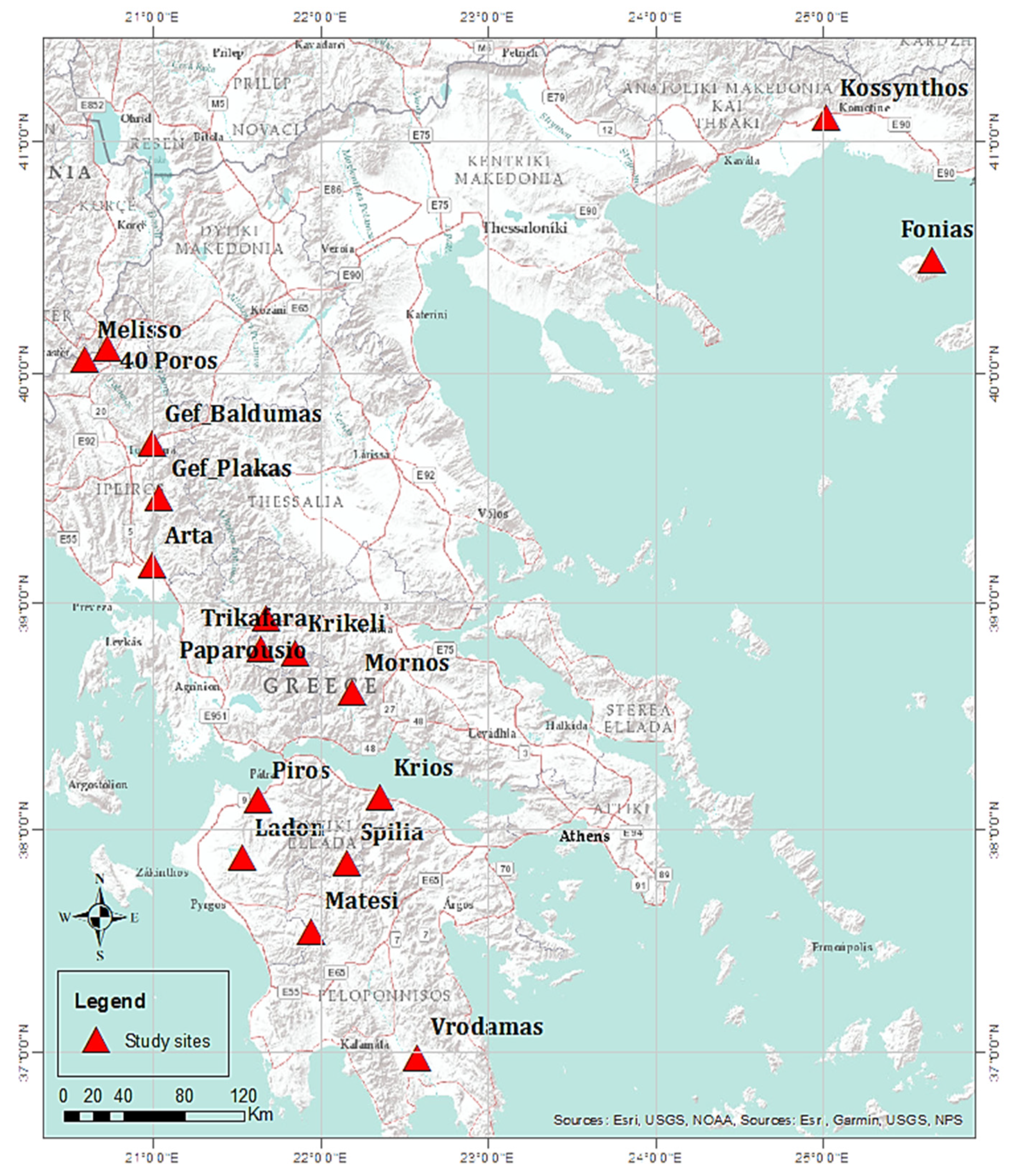
2.1. Study Area & Data Used

Incorporating the European Framework Directive 2000/60 (WFD), which established action in the field of water policy, Greece has created the National Monitoring Water Network (NMWN) to systematically and consistently gauge and monitor the quantitative and qualitative status of surface water and groundwater (http://nmwn.ypeka.gr) (accessed on 12 August 2021). The Hellenic Centre for Marine Research (HCMR) has been contracted for the monitoring of rivers and transitional and coastal waters and has been operating a large number of gauging sites across Greece. In parallel to the monitoring program, an experimental initiative has proceeded with the 3D capturing of a smaller number of selected sites [38]. Following a screening process on this shorter list of river bodies, for which both in-situ discharge measurements and 3D captures were available, 17 sites were selected and examined in this study.

The 17 selected sites are shown in Figure 1, they exhibit a considerable spatial distribution, occupying a big part of mostly mainland Greece, except for one site (Fonias), which is located on the island of Samothrace. A cluster of five sites is located in the north-western part of Greece while another cluster of four sites is located in Central Greece. Six more sites are distributed over the Peloponnese region, in southern Greece, and the other two sites are located in the north-eastern part of Greece.

Notable variations are expected in their flow regimes and other characteristics (

Table 1. General information on the 17 selected sites (name, geographic position in WGS’ 84, elevation, measured discharge and date of measurement).

Study Site Name	River/Stream Name	Latitude	Longitude	Elevation (m)	Discharge (m3/s)	Date of Measurement
40 Poros	Sarantaporos	40.11158	20.72377	416.3	1.83	Jul-2019
Arta	Aracthos	39.16543	20.99305	21.1	9.4	Jul-2019
Fonias	Fonias	40.49137	25.65514	15.0	0.05	Aug-2018
Gef_Baldumas	Dipotamos	39.69724	20.99341	437.9	0.87	Aug-2019
Gef_Plakas	Aracthos	39.45803	21.03130	230.3	11.76	Jul-2019
Kossynthos	Kossynthos	41.10172	25.02614	21.3	2.39	May-2019
Krikeli	Krikeliotis	38.77596	21.84881	827.6	0.18	Jul-2018
Krios	Krios	38.14006	22.35951	1.7	0.74	May-2019
Ladon	Pineios (Peloponnese)	37.87127	21.53456	64.2	0.48	Jul-2019
Matesi	Alfeios	37.54373	21.94867	124.2	5.0	Jul-2019
Melisso	Aoos	40.06035	20.59203	359.6	4.0	Jul-2019
Mornos	Mornos	38.60376	22.19012	487.5	1.5	Jul-2018
Paparousio	Tavropos	38.93268	21.67211	272.1	3.0	Jul-2018
Piros	Piros	38.12771	21.62715	7.7	4.35	May-2019
Spilia	Aroanios	37.84978	22.15801	418.3	2.61	Jul-2019
Trikfara	Krikeliotis	38.79830	21.64779	379.5	3.55	Jul-2018
Vrodamas	Evrotas	36.97452	22.58057	136.8	2.0	Jul-2019

), as the study sites include streams and bigger rivers alike. These variations are reflected in the measured discharge values, collected over the periods of July to August 2018 and May to August 2019 (Table 1), which range from 0.05 to 11.7 m³/s with an average of 3.2 m³/s. Considerable variations are also observed in their elevation, as values range from 1.7 to 807.6 m with an average of 248.3 m. Sites located at higher elevations comprise the first two clusters, of north-western and central Greece, since they are distributed along the Pindus mountain range and are located in fairly mountainous areas. The average elevation of these sites alone is 343.2 m. The remaining sites, located in the Peloponnese and north-eastern Greece, are located at lower elevations, with an average value of 95.8 m.

In-situ discharge measurements and UAV flights for image capturing were conducted concurrently on each site, in the spring and, for the most part, the summer months of 2018–2019. All the collected data as well as the method implemented for in-situ discharge measurement concern river segments with shallow water conditions.

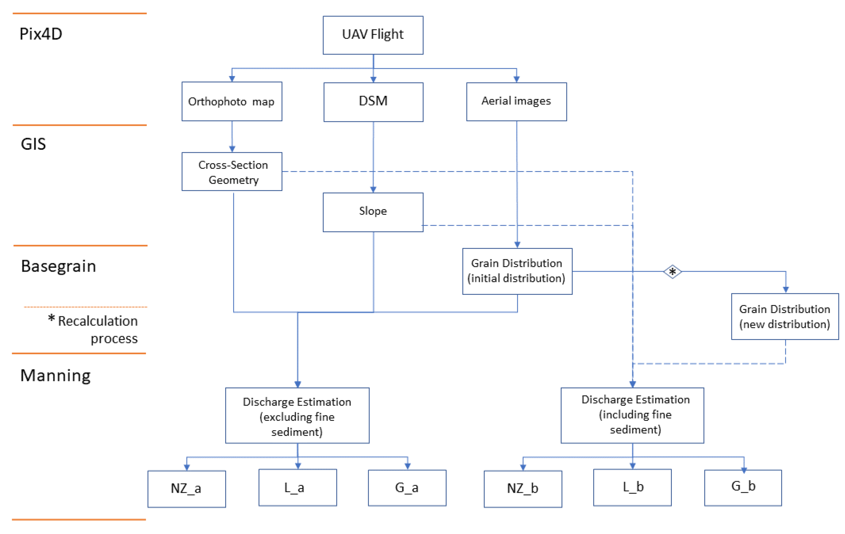
2.2. UAV Flights and Photogrammetry Software

Concerning the image capturing, the Phantom 4 pro v2.0 UAV of DJI (Shenzhen, China) was used at a certain flight altitude depending on each site’s obstacles ranging from 70 to 80 m above take off point, overall (the same altitude was maintained throughout the entire flight). The Pix4D capture mission planner (Pix4D SA, Prilly, Switzerland) was used to plan the flights above river corridors along the river course, with an 80% longitudinal and transverse image overlap and a cell size of about 2 cm/pixel. For the development of the areas’ orthophotomap and Digital Surface Model (DSM) through photogrammetry, the Pix4D mapper was used, which is a software widely applied for this purpose [39]. The relative accuracy of the produced DSM according to the software quality report was three times the cell size of the images (approximately 6 cm) while the analysis of the UAV image sensor was 20 Mpixels. The flights were recorded during the low flow periods when most of the Greek rivers have very shallow waters, and in most cases the water depth and transparency was at such levels that allowed estimation of the DSM even below the water surface. This approach provides satisfactory results when the water is very shallow and transparent [40,41].

2.3. Methodology

To begin with the proposed method, a UAV flight was performed in each site to capture the high-resolution images required. Subsequently, the images were processed to develop the orthophotomap and Digital Surface Model (DSM) of the areas. Following, a suitable river cross-section was identified on the orthophotomap and selected on each study site, for which the parameters for the Manning equation would be specified.

In a gradual process, first the geometric characteristics of a cross-section were acquired from ArcGIS utilizing both DSM and orthophotomaps produced by UAV images. Then, the UAV images of the selected cross-section were also used to estimate the riverbed particle size distribution through an automated photosieving process, which made available the initial set of distribution values. A recalculation process was also introduced, in order to account for the small size particles that were not captured in the images, and as a result, another particle size distribution was also produced. Both particle size distribution sets were examined and used in the roughness coefficient (n) estimation.

However, given that the Manning equation is especially sensitive to the roughness coefficient (n value, it was decided to use three different empirical equations for its estimation and subsequently evaluate them to define the most suitable one.

Each step incorporated in the process is separately described in the following subsections.

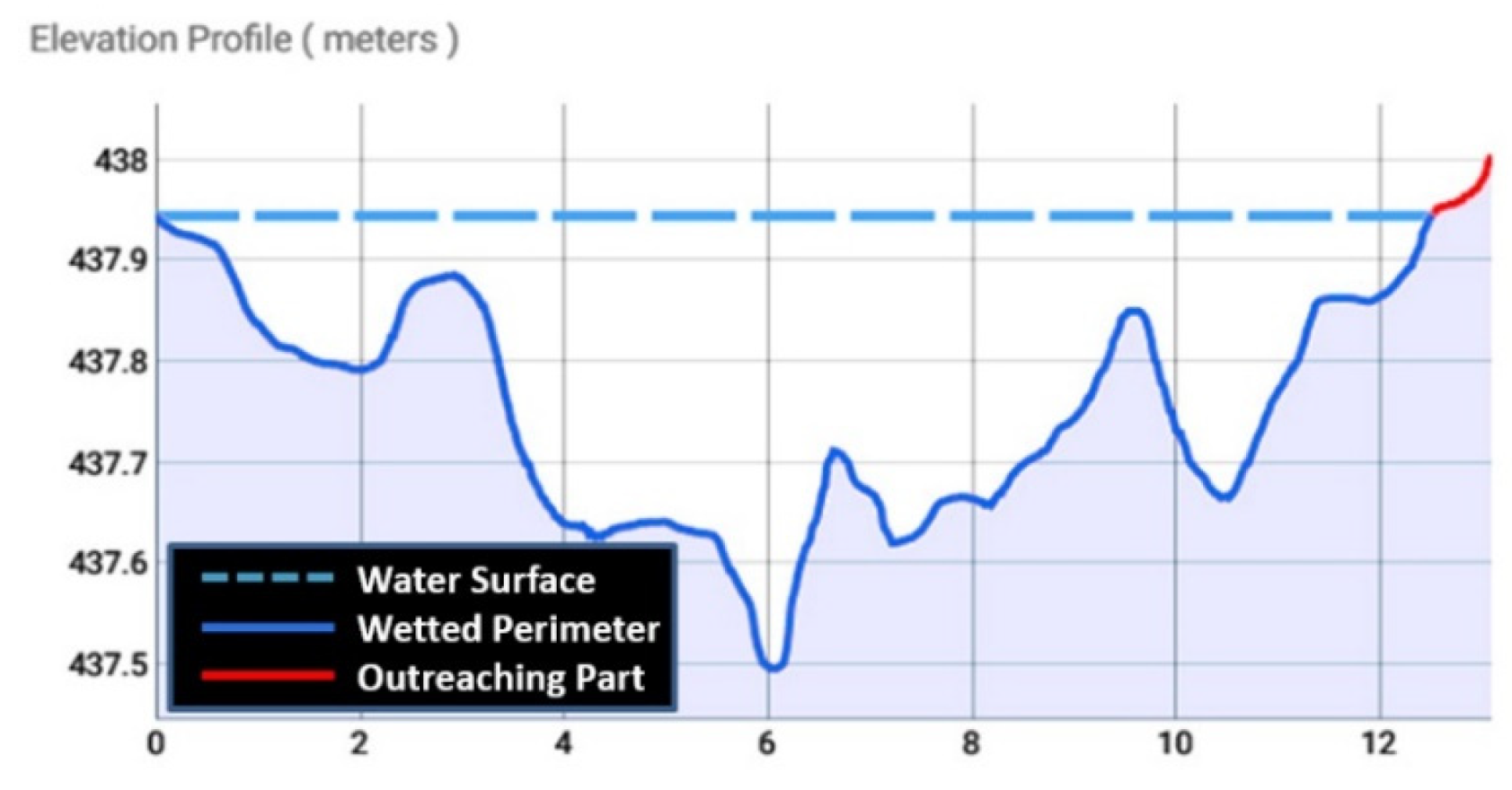
2.3.1. Cross-Section Geometry

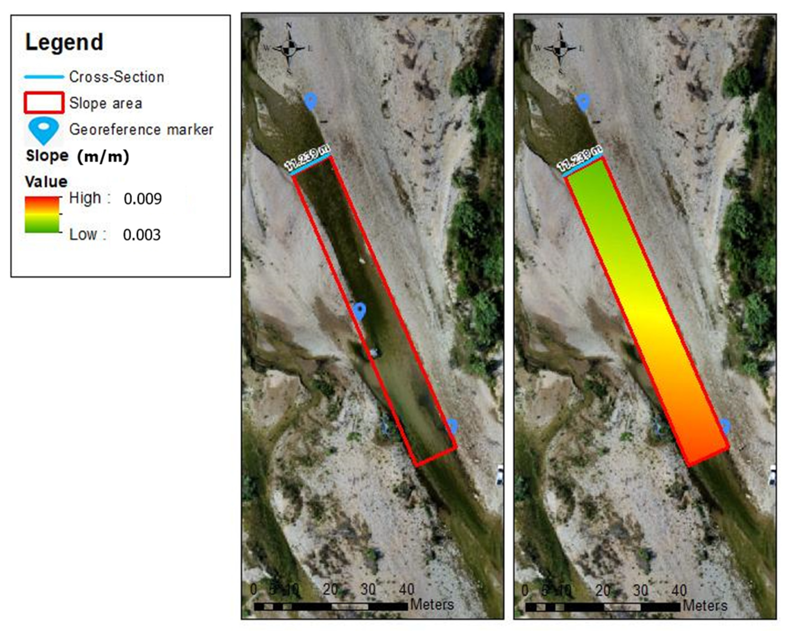
At first, a visual examination of the orthophotomap for each site was performed, to locate a suitable river segment. After numerous trial and error efforts, the suitability conditions for the selection of a representative cross-section were identified: (a) shallow water, (b) absence of vegetation covering the riverbanks, (c) image clarity, (d) water clarity and (e) cross-section positioning within a homogeneous and straight river segment. Selecting a cross-section, on which the measurements would be extracted was a challenging task as river segments that did fulfil the above set of criteria were limited in most examined cases.

Subsequently two points at the edge of the riverbanks, that would constitute a vertical section to the river flow, were selected. The elevation profile of this line was then acquired through the Pix4D platform and imported to ArcGIS software as a set of x, y points with elevation information. The resulting elevation graph was then examined to correct possible elevation discrepancies between the two points (Figure 2); the correction was always performed to the point with the highest elevation, trimming off the outreaching parts. Information on the area (A) and the wetted perimeter (P) of the cross-section created through that process could then be easily obtained via ArcGIS.

2.3.2. Slope

Measuring the gradient slope of a river can be a challenging task as its value may vary spatially and temporally to a considerable extent [17]. To overcome this difficulty, the slope value was estimated for river segments, in which uniform and steady flow conditions were assumed. In order for this assumption to be valid, an effort was made so that the selected river segments were reasonably homogeneous, non-sinuous and also long enough to make credible slope estimations. In such conditions, the water-surface slope could be approximated by the topographic slope [18,29].

These segments were represented by 2-D polygons whose vertices were selected on the edge of the riverbanks, in order to get a close approximation of the water surface (Figure 3). The one edge of the polygon was defined by the selected cross-section in each river and the other was set at a meaningful reach upwards. Depending on the specific conditions of each river, the length of this polygon varied, but in all examined sites it was never shorter than 50 m or greater than 100 m. Elevation information for the four vertices of the polygon was then extracted from the DSM, and subsequently, an interpolation method was implemented in order to acquire the slope value of the polygon.

2.3.3. Manning Roughness Coefficient

The Manning roughness coefficient (n) accounts for frictional resistance of the channel to the flow. For the estimation of n, three empirical flow dependent equations were incorporated, which make use of the measured channel substrate in natural channels. Given that each of these equations makes use of a different bed particle percentile, they were all used to estimate n, in order to examine the difference in the estimated values and define the better performing one. All three equations correlate n values with hydraulic radius and varying bed sediment sizes. Those are (for SI units):

New Zealand:

$$n=\frac{ {\mathrm{d}}_{90}{}^{1/6}}{26\left(1-{0.3595}^{{\mathrm{x}}^{0.7}}\right)}$$

(1)

Limerinos:

$$n=\frac{0.1128 R{h}^{1/6}}{1.16+2.0log \left(\frac{\mathrm{R}}{d_{84}}\right) }$$

(2)

Griffiths:

$$n=\frac{0.1128 R{h}^{1/6}}{0.76+1.98log\left(\frac{\mathrm{R}}{d_{50}}\right) }$$

(3)

where R is the hydraulic radius, d₅₀ the particle diameter of the 50th percentile of particles, d₈₄ the particle diameter of the 84th percentile of particles, d₉₀ the particle diameter for the 90th percentile of particles and x = (R/d₉₀)(d₅₀/d₉₀).

Equation (1) is the result of a modification of the Meyer-Peter and Muller equation for the determination of n, based on a detailed analysis of stream data from New Zealand conducted by Witheridge [42]. Equations (2) and (3), developed by Limerinos [43] and Griffiths [44] respectively, are well established relationships and have been widely used for the estimation of the roughness coefficient [45,46,47].

2.3.4. Riverbed Particle Size Distribution

The size-frequency characteristics used in the roughness coefficient equations are d₅₀, d₈₄ and d₉₀. Grain size distribution of bed particles was calculated with the use of the Basegrain software tool (ETH, Zurich, Switzerland) for granulometric analysis of top-view photographs of fluvial gravel beds [26]. At first, a top-view image was taken from a shallow submerged area at the selected cross-section. This image was subsequently imported and processed in Basegrain software and the bed particles size distribution was acquired through an automated photosieving process [48].

As stated above, the selected flight altitude and image sensor capabilities resulted in a resolution of approximately 20 mm/pixel. As a direct result it should be expected that the photosieving method would only be able to detect particles equal to or coarser than 20 mm. By contrast, particles classified as fine gravel and coarse sand in the images, from now on defined as fine sediment, would go undetected. Moreover, the photosieving process was influenced by additional factors such as the depth of each particle in the image, the presence of black colour or shades, etc. As a result, it is expected that, to a considerable extent, the fine sediment would not be included in the sieving analysis.

Cross-examination of the automated photosieving outcomes with the images of the orthophotomaps of river segments that in certain cases did not produce corresponding results, added to that assumption. For example, particle size distribution results proposed coarse gravel or cobble in certain study sites where a visual examination suggested that the riverbed was predominantly sand or fine gravel. Therefore, a recalculation technique was implemented to account for the fine sediment particles that went undetected. The log report of the granulometric analysis that is the output of the Basegrain procession gives the percentage of the image that was considered as grains as well as the remaining “area total void”. For the recalculation process, it was assumed that the latter percentage could be interpreted as the unaccounted-for fine sediment. Therefore, the “area total void” percentage was considered as the percentage of the particles that were below the 20 mm threshold, and on that basis, the particle size distribution of each top-view image was manually recalculated.

2.3.5. Discharge Estimation

The discharge estimations were based on the Manning formula [49], which is an empirical equation for the calculation of flow velocities in open channel flow. Discharge values were the product of the calculated flow velocity and the area of the cross-section. The Manning equation used for calculating river discharge is:

$$\mathrm{Q}=\frac{1}{n}{\mathrm{R}}^{\raisebox{1ex}{$2$}\!\left/ \!\raisebox{-1ex}{$3$}\right.}{\mathrm{S}}^{\raisebox{1ex}{$1$}\!\left/ \!\raisebox{-1ex}{$2$}\right.}\mathrm{A}$$

(4)

where Q is the estimated discharge in m³/s, n is the Manning roughness coefficient in s/m^1/3, R is the hydraulic radius in m, S is the channel slope in m/m and A is the cross-section area in m².

Eventually, the combination of the two sets of particle size distributions with the three equations for n calculation resulted in six different approaches for discharge estimation in each examined site (Figure 4).

2.4. Statistical Analysis

A statistical analysis of the results was performed to identify which combination of riverbed substrate coefficient equation and practice regarding including/excluding the fine sediment portion would produce better discharge estimations (through the Manning equation) with respect to the actual measurements. The in-situ discharge measurements were captured through the use of typical flow meters and follow the methodology described by Rantz [50]. The performance measures used were the correlation coefficient (r), root mean square error (RMSE), relative error and percentage error, along with boxplots and correlation matrices. These metrics are calculated as:

$$\mathrm{r}=\frac{n{\sum }_{i=1}^n\left(x_i{y}_i\right)-\left({\sum }_{i=1}^n{x}_i)({\sum }_{i=1}^n{y}_i\right)}{\sqrt{\left[n{\sum }_{i=1}^n{x}_i^2-{({\sum }_{i=1}^n{x}_i)}^2\right]\left[n{\sum }_{i=1}^n{y}_i^2-{({\sum }_{i=1}^n{y}_i)}^2\right]}}$$

(5)

$$RMSE=\sqrt{\sum _{i=1}^n\frac{{\left(y_{est,i}-y_{obs,i}\right)}^2}{n}}$$

(6)

$$relative error=\frac{y_{obs,i}-y_{est,i}}{y_{obs,i}}$$

(7)

$$percentage error=\frac{\left|y_{obs,i}-y_{est,i}\right|}{y_{obs,i}}\times 100$$

(8)

where $y_{est,i}$ are estimated values, $y_{obs,i}$ are observed values, $x_i,y_i$are individual sample value and n is the number of observations.

3. Results

3.1. Channel Features

Acquired values concerning the area of the cross-sections illustrated significant variations depending on the river/stream type, ranging from 0.19 to 16.5 m² with a median value of 2.5 m² (

Table 2. Chanel features and statistics of study sites.

Study Site	A (m2)	P (m)	Rh (m)	Slope (m/m)
40 Poros	1.46	9.71	0.151	0.072
Arta	5.18	21.3	0.243	0.018
Fonias	0.18	2.95	0.063	0.067
Gef_Baldumas	2.48	12.75	0.195	0.008
Gef_Plakas	16.45	46.84	0.351	0.036
Kossynthos	2.57	6.85	0.375	0.064
Krikeli	0.80	6.51	0.123	0.016
Krios	0.80	5.06	0.158	0.036
Ladon	0.93	10.92	0.085	0.006
Matesi	3.08	11.58	0.267	0.08
Melisso	13.01	30.30	0.429	0.018
Mornos	1.42	10.60	0.135	0.051
Paparousio	3.41	18.00	0.190	0.012
Piros	2.29	7.71	0.298	0.018
Spilia	3.28	7.95	0.413	0.08
Trikfara	3.49	16.62	0.210	0.011
Vrodamas	1.33	12.40	0.107	0.045
Minimum	0.18	2.95	0.063	0.006
25th percentile	1.33	7.71	0.135	0.016
Median	2.48	10.92	0.195	0.036
75th percentile	3.41	16.62	0.298	0.064
Maximum	16.45	46.84	0.429	0.08

). Respectively, wetted perimeter values fluctuated from approximately 3 to 47 m with a median value of 11 m. Similar variations were recorded for the hydraulic radius (from 0.06 to 0.43 m) and slope (from 0.006 to 0.08 m/m), indicating the great hydromorphological and hydraulic differences in the examined river bodies (Table 2).

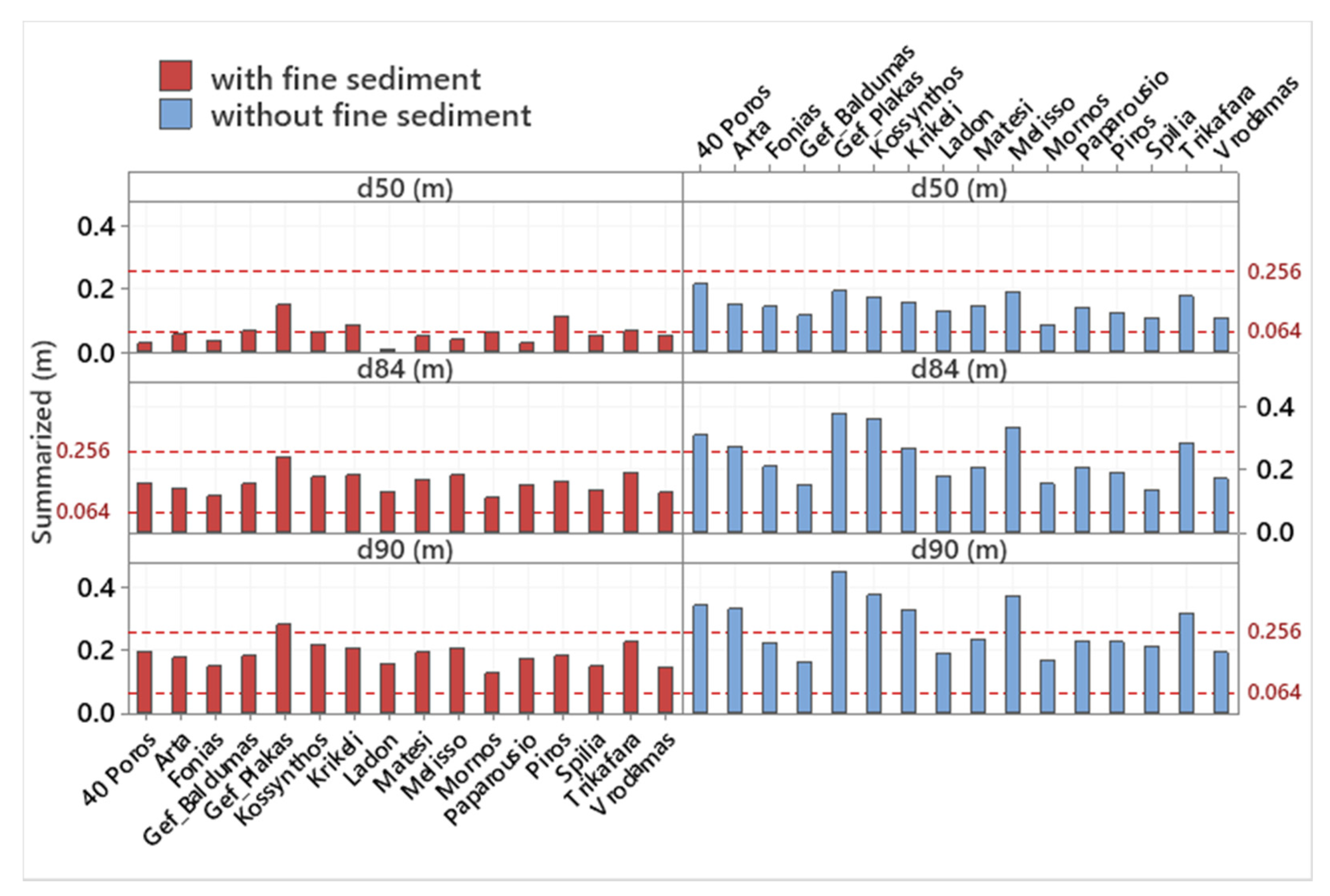
3.2. Particle Size Distribution

Results of the initial photosieving (excluding fine sediment) indicate that size parameter d₅₀ occupies values in a price range from 0.088 up to 0.215 m with a median value of 0.146 m (

Table 3. Statistics of the two riverbed particle size distributions; initial set acquired from photosieving analysis (left column) and new set from recalculation process applied (right column) to account for fine sediment.

	Initial Distribution (Excluding Fine Sediment)			Recalculated Distribution (Including Fine Sediment)
	d50 (m)	d84 (m)	d90 (m)	d50 (m)	d84 (m)	d90 (m)
Minimum	0.088	0.137	0.164	0.010	0.112	0.129
25th percentile	0.122	0.179	0.208	0.039	0.135	0.157
Median	0.146	0.208	0.233	0.055	0.157	0.184
75th percentile	0.176	0.291	0.334	0.067	0.180	0.207
Maximum	0.215	0.377	0.451	0.151	0.242	0.282
Range	0.127	0.24	0.287	0.141	0.13	0.153

). Recorded values for the d₈₄ parameter vary from 0.137 to 0.377 m with a median of 0.240 m, while the respective values for the d₉₀ parameter range from 0.164 m to 0.451 m with a median of 0.233 m. Following the implementation of the recalculation process, which aimed to account for the fine sediment, the photosieving results were significantly modified and values concerning all examined particle size parameters were decreased considerably (Figure 5). Size parameter d₅₀ recorded values as low as 0.010 m and up to 0.151 m with a median of 0.055 m (62.3% decrease). Considerable alteration resulted also in both the d₈₄, which fluctuated from 0.112 m up to 0.242 m with a median of 0.157 m (24.5% decrease), and the d₉₀, which ranged from 0.129 m to 0.282 m with a median of 0.184 m (21.0% decrease). The value range was also considerably decreased after the recalculation process, especially for the d₈₄ (from 0.24 to 0.13 m) and d₉₀ (from 0.287 to 0.153 m) parameters.

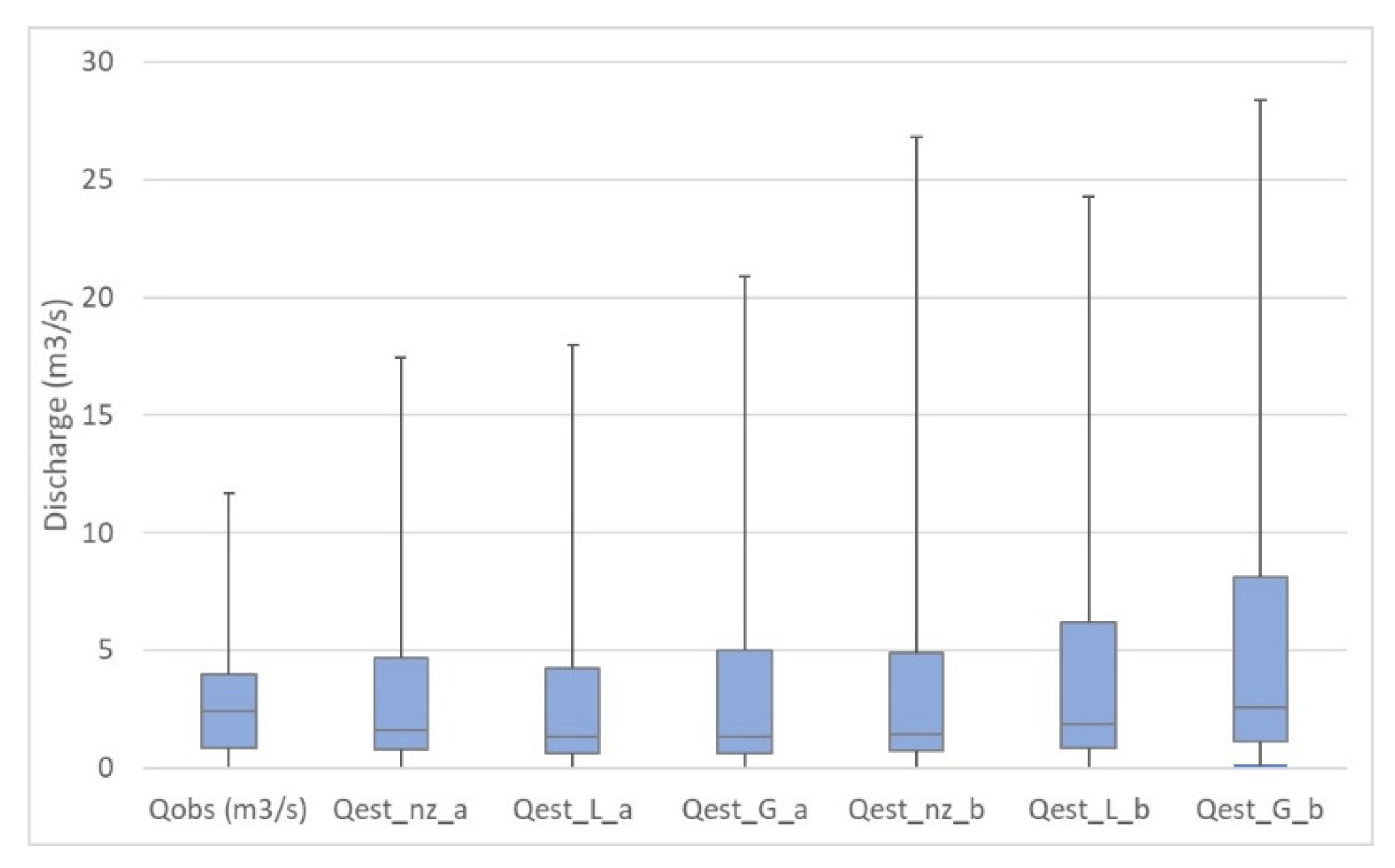
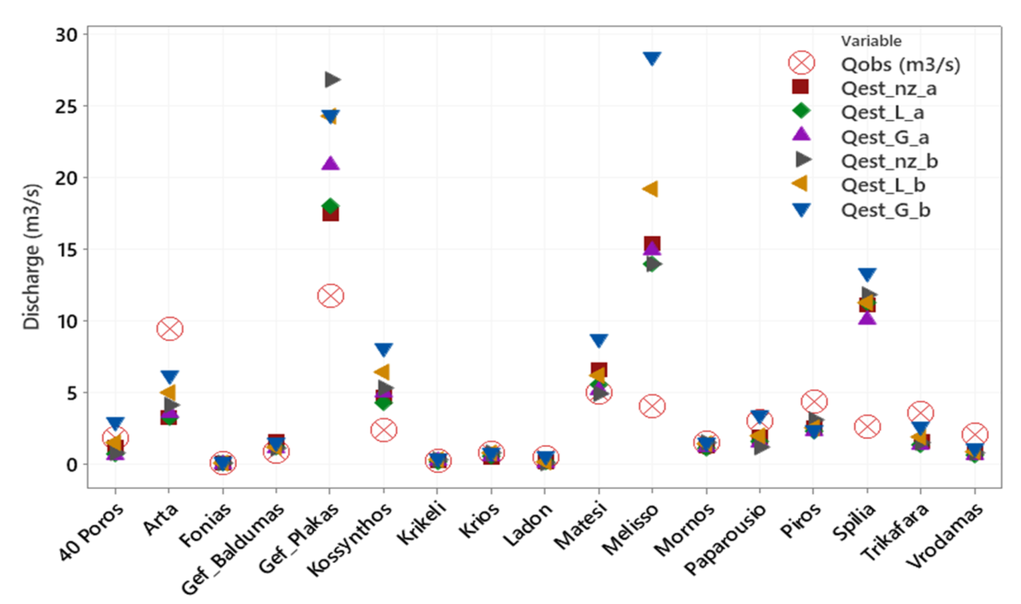
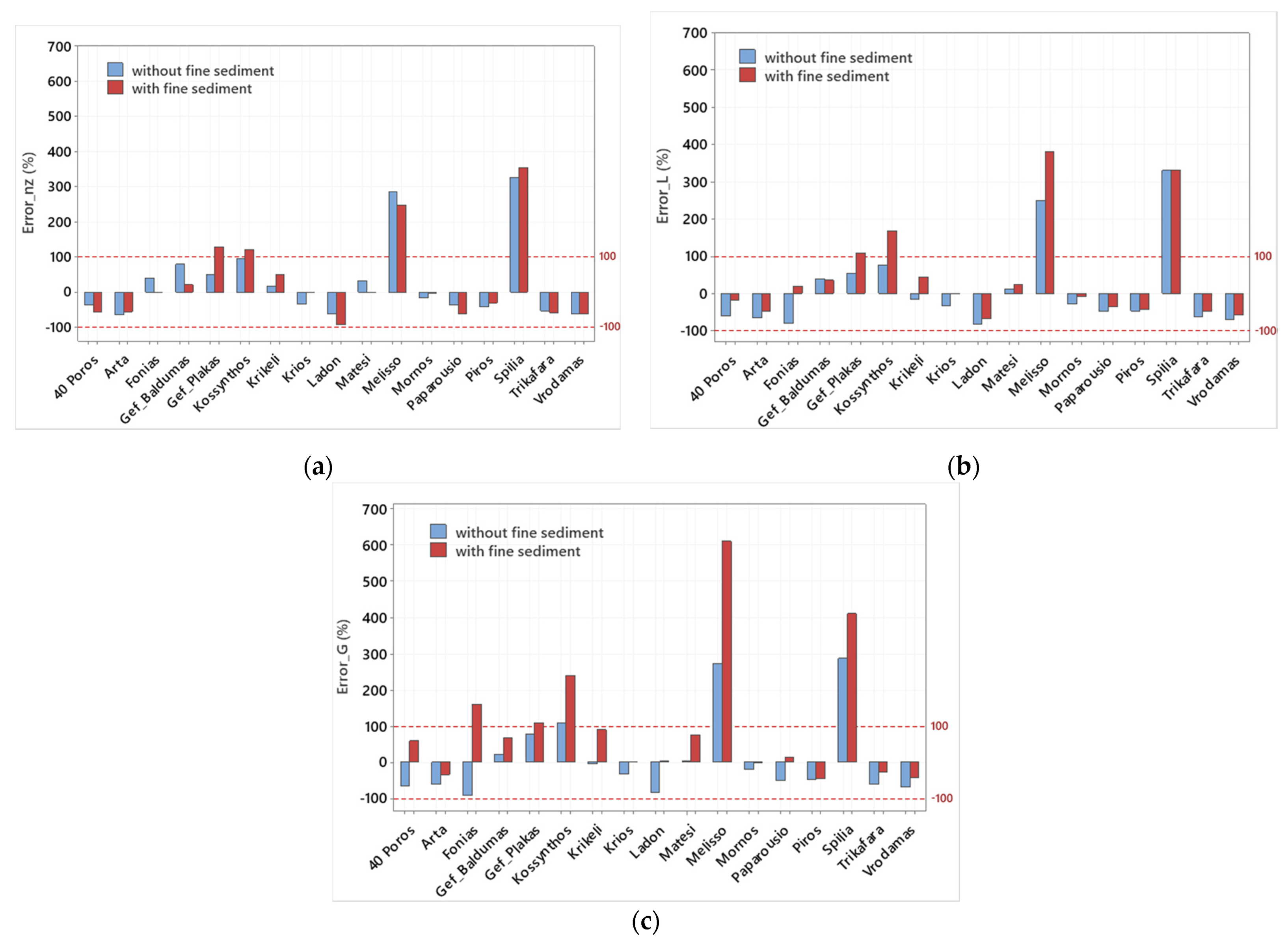
3.3. Discharge Estimation

Discharge estimations in the study sites indicated that Limerinos and New_Zealand approaches performed slightly better, regardless of including or not the fine sediment portion, while the Griffiths method indicated relatively good performance in approximately 50% of the sites and had significant errors in the rest (

Table 4. Measured discharge (Qobs) versus the estimated discharge values for all six different approaches, in m³/s.

	Qobs	Initial Distribution (Excluding Fine Sediment)			Recalculated Distribution (Including Fine Sediment)
Estimation method		New_Zealand	Limerinos	Griffiths	New_Zealand	Limerinos	Griffiths
Minimum	0.05	0.07	0.01	0.00	0.04	0.06	0.13
25th percentile	0.87	0.78	0.62	0.61	0.75	0.83	1.12
Median	2.39	1.63	1.34	1.35	1.46	1.85	2.58
75th percentile	4.00	4.68	4.23	5.00	4.91	6.19	8.11
Maximum	11.70	17.43	18.00	20.89	26.81	24.31	28.39

, Figure 6). Three approaches, the L_a, G_a and NZ_b, estimated most of the discharges within the 0–5 m³/s range, similar to the range of the measured discharges. However, all three methods produced some significant overestimations in certain sites. The three remaining approaches, NZ_a, L_b and G_b, produced estimations within a wider range (0–10 m³/s) as well as more extreme overestimation values. In addition, the higher overestimations were produced when the fine sediment was included for all three (Limerinos, Griffiths and New_Zealand) methods.

There are 12 sites (75% of total) for which the discharge estimation is satisfactory (less than 50% estimation error) using at least one of the approaches tested and four sites with significant deviations (more than 50% estimation error) from the in-situ measurements for all methodological approaches (Figure 7). Additionally, there are 10 sites for which the discharge estimation is pretty accurate for all six methods applied.

In all methodological approaches applied in this study, four sites (Melisso, Spilia, Kossynthos and Gef_Plakas) were found to always have significant errors in their estimated discharge values compared to the in-situ discharge measurements. In order to identify a potential justification of their underperformance, further examination of these high-error sites through a statistical analysis of the geometric and hydraulic characteristics of their cross-sections was conducted. Results illustrated a significant correlation, of r = 0.72 with a p-value of 0.001, between the Rh and the percentage error values (

Table 5. Correlation coefficient matrix of different cross-section physical characteristics as an average of the percentage error per site of the six discharge estimation approaches.

	A (m2)	P (m)	Rh (m)	Slope (m/m)
Average Error (%)	0.44	0.22	0.72	0.19

). The results suggest that a threshold in the Rh value exists, approximately at 0.3 m or slightly above this value; sites with Rh reaching over that threshold value produced high errors in the estimated discharge. The four high error sites are all, to a smaller or greater extent, above the Rh threshold of Rh = 0.3 m, with an average value of 0.392 m. The remaining 13 sites, in which at least one approach of the implemented discharge estimation produced good results, have a significantly lower average Rh of 0.171 m. The rest of the examined features of the four sites (A, P, S) did not show any considerable correlation to the average percentage error (

Table 6. Estimated RMSE for all six approaches for discharge estimation, where RMSE_T1 is calculated for all 17 sites, RMSE_T2 is calculated without the four high error sites, nz = New_Zealand, L = Limerinos, G = Griffiths, a = initial particle size distribution and b = recalculated particle size distribution.

	NZ_a	L_a	G_a	NZ_b	L_b	G_b
RMSE_T1	4.14	3.98	4.31	5.21	5.49	7.41
RMSE_T2	1.99	2.02	1.95	1.77	1.52	1.56

).

The RMSE was estimated twice for each of the six approaches, using two different sets of discharge values in each case (Table 6). The first method (RMSE_T1) included discharge values from all 17 sites, while the second (RMSE_T2) omitted discharge values from the four high error sites (Melisso, Spilia, Kossynthos, Gef_Plakas). For RMSE_T1, Limerinos, excluding fine sediment had the lower RMSE value (3.98 m³/s), while the higher RMSE value was observed at Griffiths including fine sediment (7.4 m³/s). However, it should be noted that, as a whole, these RMSE values have a considerably high range (4.0–7.4 m³/s) in comparison to the range of the discharge values from the in-situ measurements. For RMSE_T2 the new error values were significantly better overall; for all six approaches they ranged from 1.5 to 2.0 m³/s, while the better performing method proved to be Limerinos including fine sediment (1.52 m³/s).

With respect to error percentages (% deviation from measurement) Griffiths and Limerinos methods had the absolute lowest values when fine sediment was excluded from the analysis while New_Zealand and Limerinos had the lower median and 75th percentile errors (

Table 7. Percentage error of discharge estimations, with and without fine sediment particle distribution.

	Initial Distribution (Excluding Fine Sediment)			Recalculated Distribution (Including Fine Sediment)
	New_Zealand	Limerinos	Griffiths	New_Zealand	Limerinos	Griffiths
Minimum	16.8%	10.9%	2.0%	0.7%	7.8%	1.2%
25th percentile	35.9%	37.8%	21.4%	30.4%	35.2%	27.3%
Median	54.2%	60.6%	62.2%	58.7%	44.9%	58.4%
75th percentile	79.5%	76.6%	84.6%	116.4%	69.4%	107.1%
Maximum	326.9%	330.0%	286.7%	353.2%	380.4%	609.7%

). When the fine sediment portion was included in the analysis, New_Zealand and Griffiths methods had the lower minimum and 25th percentile errors while Limerinos and Griffiths had the lower median and 75th percentile errors. Including the fine sediment portion in the analysis improved results and decreased percentage errors in more than 50% of the rivers but increased the errors significantly in approximately 25% of the rivers with the highest deviations between discharge estimates and measurements. Taking into account all sites, no specific approach could be distinguished as better performing overall. However, it can be stated that the worst performing approach is Griffiths including fine sediment, which scored the two highest estimation errors (409.3% and 609.7%). When the four high error sites (mentioned in the above paragraph) were excluded, Limerinos and New_Zealand including the fine sediment had the lowest average error percentages, scoring 34.6% and 38.0%, respectively. Yet, the impact of including or excluding the fine sediment portion in the discharge estimation is not very obvious in terms of errors because it is contradictory from one method to the other, but in the best performing method (Limerinos) including fine sediment in the analysis has a positive effect.

By using the New_Zealand method, underestimation of discharge was observed in 9 out of the 17 rivers, while the percentage error exceeded +100% in 4 sites (24% of total). Including the fine sediment portion in the estimation process improved the results by reducing percentage error in 7 sites (42% of the total) (Figure 8a). The highest errors were observed in Melisso and Spilia rivers, followed by Gef_Plakas and Kossynthos. With the Limerinos method (Figure 8b), slight underestimation of discharge was observed in 11 out of 17 sites (65% of total), while errors higher than 100% were observed in 4 sites (24% of total). Including fine sediment in the analysis increased the estimation accuracy in 11 sites (65% of total), which is a significant improvement in the results. The highest errors were again recorded in Melisso and Spilia sites. Griffiths’ method (Figure 8c) illustrated the highest errors with 5 out of 17 sites (29% of total) exceeding the 100% error margin while in 10 sites (59% of total) underestimation of discharge was observed. Moreover, in 9 out of 17 sites (53% of total) including fine sediment in the analysis improved the results by decreasing errors.

The correlation matrix of the hydraulic characteristics and the discharge measurements and estimations according to the various methodological approaches indicate that both estimated and measured discharge are strongly correlated with the cross-section area and wetted perimeter (

Table 8. Correlation matrix of hydraulic characteristics, discharge measurements and discharge estimations.

	A (m2)	P (m)	Rh (m)	Slope (m/m)	Qobs (m3/s)
P (m)	0.948
Rh (m)	0.653	0.456
Slope (m/m)	−0.161	−0.289	0.147
Qobs (m3/s)	0.764	0.804	0.529	−0.07
Qest_nz_a (m3/s)	0.9	0.757	0.826	0.153	0.645
Qest_L_a (m3/s)	0.901	0.767	0.81	0.149	0.664
Qest_G_a (m3/s)	0.932	0.812	0.779	0.108	0.696
Qest_nz_b (m3/s)	0.915	0.817	0.729	0.115	0.729
Qest_L_b (m3/s)	0.943	0.82	0.784	0.095	0.695
Qest_G_b (m3/s)	0.919	0.773	0.809	0.083	0.611

). Hydraulic radius is also strongly correlated with the estimated discharges but not with the measured ones on all approaches, while slope values present very low correlation coefficients with all estimated and measured discharges. The observed discharges are better correlated (r = 0.729) to discharges estimated with the New_Zealand method including the fine sediment portion (RMSE = 1.77 m³/s), while the lowest correlation with the measured values comes from estimates using the Griffiths method, including fine sediment (RMSE = 1.56 m³/s) (Table 8).

4. Discussion

4.1. Discharge Estimation

The results of this study showed that in most cases (almost 75% of sites) at least one of the six methods used for discharge estimation produced good results (less than 50% estimation error). Four sites were found to always produce significant estimation errors independently of the approach implemented. Further examination proposed that the errors should rather be attributed to the selected cross-section characteristics than the estimation methods used. Moreover, 10 out of the 17 study sites (58.8%) produced accurate discharge approximation for all six approaches alike. These accounts imply that the process proposed for discharge estimation, incorporating UAV images combined with empirical hydraulic equations, can offer a credible alternative for discharge measurements under specific conditions, primarily shallow water conditions.

As a general rule, Limerinos and New_Zealand proved to have better performances in most sites, with small estimation errors and small RMSE values. The New_Zealand approach excluding fine sediment had good estimations (less than 50% error) in 8 sites. The fine sediment recalculation had a positive effect especially for the Limerinos approach, in which the estimation accuracy was increased in 11 sites (65% of total) and proved to be the best performing method. Contrarily, the worst performing method was Griffiths after the fine sediment recalculation, which produced the highest average error (1171%) and the highest RMSE (7.41 m³/s) for all sites combined and the highest error of an individual site (6097% for Melisso), for all six approaches and sites examined. Nevertheless, amongst the six different discharge estimation approaches tested in this study, no single one proved to significantly outperform the others. Their performance was to a considerable extent site specific, proposing that different equations have better applicability on certain sites, most likely a matter related to the sites’ physical characteristics. In addition, the recalculation process of particle size distribution, which was implemented in order to account for the fine sediment, did not have a consistent positive impact on all approaches and throughout every study site. Finally, a strong correlation between average error in discharge estimation and Rh was highlighted. Results propose that a threshold value of 0.3 m exists; sites equalling or exceeding it are expected to produce high errors.

Regarding the RMSE (Table 6), when all sites were included in its calculation (RMSE_T1) all six approaches scored high error values, suggesting that no single approach can be uniformly and indiscriminately used in all examined sites. It was presumed that the RMSE metric was getting significantly distorted from the four high error sites, for which the discharge estimation process proved not applicable. Therefore, new error values could be calculated from the sites in which the estimation method was at least applicable, even if it did not produce good (below 50% estimation error) results. From that perspective, it was decided that the four high error sites should be omitted from the new RMSE calculation process. The RMSE_T2 produced considerably better results, ranging from 1.5 to 2.0 m³/s, closer to the order of magnitude of the discharge values in most of the examined sites. It is also interesting to note that when all sites were used in the RMSE calculation, the smaller values were scored by the approaches that excluded fine sediment. Contrarily, when the four high error sites were omitted from the calculation process, the smaller RMSE values were scored for the three approaches including fine sediment. This observation could suggest that, for sites where the proposed method of discharge estimation is applicable (not exceeding 100% estimation error), the fine sediment recalculation process has a positive impact.

The results of this study are comparable to those from Yang et al. [15] who made use of UAV-acquired data as well as three different equations of the slope-area method for discharge calculation and produced an overall qualification rate of 70% for the calculated discharge. Similarly to this study, there was not a specific equation outperforming the others; the applicability of each equation was rather dependent on the discharge characteristics of each site. Quite alike, Yang et al. [15] also highlighted the importance of Rh in the discharge estimation process. Furthermore, Zhao et al. [28] proposed a new framework coupling the virtual hydraulic radius (VHR) with the modified global at-many-stations hydraulic geometry (global-AMHG) method and UAV imagery, through which it was possible to yield significantly higher accuracy for streamflow estimation of medium-to-small scale rivers. Recently, Eltner et al. [51] followed an automated workflow on UAV imagery for surface flow velocity calculation combined with photogrammetry-derived cross-section geometry to estimate discharge in rivers, with deviation from measured discharge up to 31%.

4.2. Recalculating Particle Size Distribution

Implementation of the recalculating process significantly affected the particle size distribution, in most study sites. The effects of the recalculation were more evidently manifested in the case of the d₅₀ parameter. Having an initial median size (0.151 m) according to which d₅₀ was classified in the cobble category, this parameter was considerably decreased after fine sediment inclusion (new median size of 0.055 m) and was reclassified into the gravel category (Table 3). For d₈₄ and d₉₀, the recalculation process produced moderate changes in their median size but was better manifested in their 75th percentile and maximum values. Judging by their maximum values, both parameters were reclassified by one order of magnitude, i.e., from boulder to cobble category. As expected, these alterations had significantly influenced the outcomes of the n value for Equations (1)–(3).

The recalculation process improved the discharge estimation for all methods but to a different extent for each of them. It proved that the best results were observed for the Limerinos method, with improved results in 65% of sites, followed by the New_Zealand method, scoring a respective improvement in 42% of sites. Nevertheless, from site to site and from method to method, the effects of the recalculation process are not consistent. Issues with the applicability of each method for every site and the sensitivity of the discharge estimation to the n value could most likely be reasons for this inconsistency. However, a solid conclusion on the effect of the recalculation process could not be drawn and further examination is needed on this matter.

4.3. Additional Sources of Error

Errors in the estimated discharges should not be sought unilaterally on weaknesses of the proposed method, as different sources of uncertainty also exist. Namely, in the empirical hydraulic equations used in this study, the discharge estimation is a function of diverse parameters, such as A, P, S, n. Therefore, it is expected that uncertainties when estimating their values will introduce errors, sincethe estimates of hydraulic characteristics of the cross-section extracted by both remote sensing and in-situ measurements often incorporate relatively high errors, as various studies have indicated [52,53]. Some of the uncertainties of remote sensing, include factors such as the UAV camera angle, UAV flight height and light intensity, as well as effects from refraction and irregularities of natural riverbed under submerged sections. Uncertainties from in-situ measurements are also expected since field measurements are conducted by different teams under varying river conditions and equipment (current meters, portable Doppler, radars, etc.).

4.4. Conditions of Applicability

Statistical analysis of the discharge estimations and the hydraulic characteristics of the cross-sections suggested a strong correlation between high errors and Rh. The performed analysis defined a threshold value of approximately Rh = 0.3, proposing that sites equalling or exceeding this value are expected to produce high errors. High Rh values could result either from high A or low P of a cross-section, both being indicators of deep-water conditions. This observation is in agreement with the claim that the proposed method is rather suitable for shallow water conditions. A possible explanation for this observation could be that deep water conditions hamper the UAV image sensor from capturing the river bottom and result in reduced precision of the elevation measurements, ultimately affecting the estimated discharge value. This finding is in accordance with Woodget et al. [54] who studied submerged fluvial topography using high resolution unmanned aerial system (UAS) imagery and concluded that DEM error in submerged river parts is depth-dependent and that the two are positively correlated. Therefore, it is proposed that the developed method for discharge estimation should be applied in cross-sections that do not exceed the Rh = 0.3 m threshold.

Additionally, several trial-and-error efforts demonstrated that the selection of a representative river segment as well a suitable cross-section on which the proposed method would be implemented are of key importance. A set of different parameters seems to define the suitability of the selected site and cross-section. The first criteria proved to be water depth; the selected cross-section should be in relatively shallow water, as deep water conditions add to measurement error [54]. Secondly, river sections with high vegetation coverage should be avoided since trees or bushes covering the riverbanks impede the actual terrain measurements. The third crucial parameter was image and water clarity. As expected, it was observed that turbidity of water affects the accuracy of the riverbed elevation measurement decisively. Turbidity could be a result of natural processes, such as sediment transportation, but could also be the result of manmade pollution. However, even in water clarity conditions, parts of an image could be inadequate for extraction of elevation information due to surface roughness. For example, riffles or high turbulence water sections of a river should be avoided as they result in cross-section irregularities and unrealistic elevation spikes. The same effect was observed in areas with intense sunlight reflections on the water surface. Finally, to facilitate both the processes of slope determination as well as the roughness coefficient estimation, another crucial parameter proved to be the selection of a cross-section at the end of a relatively homogeneous and straight river segment rather than a sinuous one.

Despite the gains from the growing use of UAVs for environmental remote sensing in the last few years and their continuous technological advancements, there are still important limitations related to their operation and processing. Weather conditions such as strong winds [55], rain [56] and air temperature [57] are major constraints that can alter the quality of surveys. In addition, the flight time of a UAV and consequently the temporal resolution of a mission are fundamentally limited by battery capacity and their quick depletion, an issue addressed by many researchers [58,59,60]. A set of other shortcomings is related to the fact that general market digital cameras are used for photogrammetry and remote sensing, resulting in illumination issues, image classification and relief displacement problems [61]. Finally, issues such as the data processing being left to the final user [62] and the high demand on data storage and processing [63] are also significant limitations.

5. Conclusions

Using UAV products and photogrammetric approaches to estimate discharge in shallow rivers can provide an efficient solution for monitoring ungauged and difficult to access rivers, with an affordable and reliable methodology. With a considerably high rate of 75% of the examined sites, at least one of the implemented approaches produced good results for discharge estimation. In addition, in 10 out of 17 sites (58.8%) all implemented approaches had very accurate approximation of the measured discharge. A recalculation process, to include fine sediment in the estimation process, was also introduced, which proved to have a positive effect on sites with small estimation error, by significantly reducing the RMSE. Overall, however, the recalculation process generated diverse results and additional investigation is needed on the matter. Finally, a strong correlation between high errors for sites exceeding an Rh = 0.3 m threshold value was observed. Based on the aforementioned results, it has become obvious that the proposed methodology for discharge estimation is more suitable for shallow water conditions.

Further research should be conducted to justify and optimize the methodological approaches for the above task but the potential for acquiring large volumes of crucial hydrologic data exist and is expected to improve water management and restoration efforts in the near future.

References

1. Dixon, H.; Hannaford, J.; Fry, M.J. The Effective Management of National Hydrometric Data: Experiences from the United Kingdom. Hydrol. Sci. J. 2013, 58, 1383–1399. [Google Scholar] [CrossRef] [Green Version]
2. Irving, K.; Kuemmerlen, M.; Kiesel, J.; Kakouei, K.; Domisch, S.; Jähnig, S.C. A High-Resolution Streamflow and Hydrological Metrics Dataset for Ecological Modeling Using a Regression Model. Sci. Data 2018, 5, 180224. [Google Scholar] [CrossRef]
3. Blöschl, G. Predictions in Ungauged Basins—Where Do We Stand? Proc. IAHS 2016, 373, 57–60. [Google Scholar] [CrossRef] [Green Version]
4. McGlynn, B.L.; Blöschl, G.; Borga, M.; Bormann, H.; Hurkmans, R.; Komma, J.; Nandagiri, L.; Uijlenhoet, R.; Wagener, T. A Data Acquisition Framework for Prediction of Runoff in Ungauged Basins. In Runoff Prediction in Ungauged Basins, Synthesis across Processes, Places, and Scales; Cambridge University Press: Cambridge, UK; pp. 29–52.
5. Gaume, E.; Bain, V.; Bernardara, P.; Newinger, O.; Barbuc, M.; Bateman, A.; Blaškovičová, L.; Blöschl, G.; Borga, M.; Dumitrescu, A.; et al. A Compilation of Data on European Flash Floods. J. Hydrol. 2009, 367, 70–78. [Google Scholar] [CrossRef] [Green Version]
6. Marchi, L.; Borga, M.; Preciso, E.; Gaume, E. Characterisation of Selected Extreme Flash Floods in Europe and Implications for Flood Risk Management. J. Hydrol. 2010, 394, 118–133. [Google Scholar] [CrossRef]
7. Mertes, L.A.K. Remote Sensing of Riverine Landscapes: Remote Sensing of Riverine Landscapes. Freshw. Biol. 2002, 47, 799–816. [Google Scholar] [CrossRef]
8. Bowen, Z.H.; Waltermire, R.G. Evaluation of Light Detection and Ranging (Lidar) for Measuring River Corridor Topography. J. Am. Water Res. Assoc. 2002, 38, 33–41. [Google Scholar] [CrossRef]
9. Parsons, D.R.; Best, J.L.; Orfeo, O.; Hardy, R.J.; Kostaschuk, R.; Lane, S.N. Morphology and Flow Fields of Three-Dimensional Dunes, Rio Paraná, Argentina: Results from Simultaneous Multibeam Echo Sounding and Acoustic Doppler Current Profiling: Three-Dimensional Alluvial Dunes, Rio Paraná. J. Geophys. Res. 2005, 110. [Google Scholar] [CrossRef] [Green Version]
10. Heritage, G.; Hetherington, D. Towards a Protocol for Laser Scanning in Fluvial Geomorphology. Earth Surf. Process. Landf. 2007, 32, 66–74. [Google Scholar] [CrossRef]
11. Bjerklie, D.M.; Birkett, C.M.; Jones, J.W.; Carabajal, C.; Rover, J.A.; Fulton, J.W.; Garambois, P.-A. Satellite Remote Sensing Estimation of River Discharge: Application to the Yukon River Alaska. J. Hydrol. 2018, 561, 1000–1018. [Google Scholar] [CrossRef] [Green Version]
12. Gleason, C.; Durand, M. Remote Sensing of River Discharge: A Review and a Framing for the Discipline. Remote Sens. 2020, 12, 1107. [Google Scholar] [CrossRef] [Green Version]
13. Lou, H.; Wang, P.; Yang, S.; Hao, F.; Ren, X.; Wang, Y.; Shi, L.; Wang, J.; Gong, T. Combining and Comparing an Unmanned Aerial Vehicle and Multiple Remote Sensing Satellites to Calculate Long-Term River Discharge in an Ungauged Water Source Region on the Tibetan Plateau. Remote Sens. 2020, 12, 2155. [Google Scholar] [CrossRef]
14. Huang, Q.; Long, D.; Du, M.; Zeng, C.; Qiao, G.; Li, X.; Hou, A.; Hong, Y. Discharge Estimation in High-Mountain Regions with Improved Methods Using Multisource Remote Sensing: A Case Study of the Upper Brahmaputra River. Remote Sens. Environ. 2018, 219, 115–134. [Google Scholar] [CrossRef]
15. Yang, S.; Wang, P.; Lou, H.; Wang, J.; Zhao, C.; Gong, T. Estimating River Discharges in Ungauged Catchments Using the Slope–Area Method and Unmanned Aerial Vehicle. Water 2019, 11, 2361. [Google Scholar] [CrossRef] [Green Version]
16. Bandini, F.; Lüthi, B.; Peña-Haro, S.; Borst, C.; Liu, J.; Karagkiolidou, S.; Hu, X.; Lemaire, G.G.; Bjerg, P.L.; Bauer-Gottwein, P. A Drone-Borne Method to Jointly Estimate Discharge and Manning’s Roughness of Natural Streams. Water Res. 2021, 57. [Google Scholar] [CrossRef]
17. Bjerklie, D.M.; Lawrence Dingman, S.; Vorosmarty, C.J.; Bolster, C.H.; Congalton, R.G. Evaluating the Potential for Measuring River Discharge from Space. J. Hydrol. 2003, 278, 17–38. [Google Scholar] [CrossRef]
18. Bjerklie, D.M.; Moller, D.; Smith, L.C.; Dingman, S.L. Estimating Discharge in Rivers Using Remotely Sensed Hydraulic Information. J. Hydrol. 2005, 309, 191–209. [Google Scholar] [CrossRef]
19. Birkinshaw, S.J.; Moore, P.; Kilsby, C.G.; O’Donnell, G.M.; Hardy, A.J.; Berry, P.A.M. Daily Discharge Estimation at Ungauged River Sites Using Remote Sensing. Hydrol. Process. 2014, 28, 1043–1054. [Google Scholar] [CrossRef]
20. Bonnema, M.G.; Sikder, S.; Hossain, F.; Durand, M.; Gleason, C.J.; Bjerklie, D.M. Benchmarking Wide Swath Altimetry-Based River Discharge Estimation Algorithms for the Ganges River System. Water Resour. Res. 2016, 52, 2439–2461. [Google Scholar] [CrossRef] [Green Version]
21. Gleason, C.J.; Smith, L.C.; Lee, J. Retrieval of River Discharge Solely from Satellite Imagery and At-Many-Stations Hydraulic Geometry: Sensitivity to River Form and Optimization Parameters. Water Resour. Res. 2014, 50, 9604–9619. [Google Scholar] [CrossRef]
22. Wu, H.; Li, Z.-L. Scale Issues in Remote Sensing: A Review on Analysis, Processing and Modeling. Sensors 2009, 9, 1768–1793. [Google Scholar] [CrossRef]
23. Anderson, K.; Gaston, K.J. Lightweight Unmanned Aerial Vehicles Will Revolutionize Spatial Ecology. Front. Ecol. Environ. 2013, 11, 138–146. [Google Scholar] [CrossRef] [Green Version]
24. Vivoni, E.R.; Rango, A.; Anderson, C.A.; Pierini, N.A.; Schreiner-McGraw, A.P.; Saripalli, S.; Laliberte, A.S. Ecohydrology with Unmanned Aerial Vehicles. Ecosphere 2014, 5, 130. [Google Scholar] [CrossRef] [Green Version]
25. Vélez-Nicolás, M.; García-López, S.; Barbero, L.; Ruiz-Ortiz, V.; Sánchez-Bellón, Á. Applications of Unmanned Aerial Systems (UASs) in Hydrology: A Review. Remote Sens. 2021, 13, 1359. [Google Scholar] [CrossRef]
26. Detert, M.; Johnson, E.D.; Weitbrecht, V. Proof-of-concept for Low-cost and Non-contact Synoptic Airborne River Flow Measurements. Int. J. Remote Sens. 2017, 38, 2780–2807. [Google Scholar] [CrossRef]
27. Lewis, Q.W.; Lindroth, E.M.; Rhoads, B.L. Integrating Unmanned Aerial Systems and LSPIV for Rapid, Cost-Effective Stream Gauging. J. Hydrol. 2018, 560, 230–246. [Google Scholar] [CrossRef]
28. Zhao, C.S.; Pan, T.L.; Xia, J.; Yang, S.T.; Zhao, J.; Gan, X.J.; Hou, L.P.; Ding, S.Y. Streamflow Calculation for Medium-to-Small Rivers in Data Scarce Inland Areas. Sci. Total Environ. 2019, 693, 133571. [Google Scholar] [CrossRef]
29. Kang, B.; Kim, J.G.; Kim, D.; Kang, D.H. Flow Estimation Using Drone Optical Imagery with Non-Uniform Flow Modeling in a Controlled Experimental Channel. KSCE J. Civ. Eng. 2019, 23, 1891–1898. [Google Scholar] [CrossRef]
30. Kinzel, P.; Legleiter, C. SUAS-Based Remote Sensing of River Discharge Using Thermal Particle Image Velocimetry and Bathymetric Lidar. Remote Sens. 2019, 11, 2317. [Google Scholar] [CrossRef] [Green Version]
31. Fulton, J.W.; Anderson, I.E.; Chiu, C.-L.; Sommer, W.; Adams, J.D.; Moramarco, T.; Bjerklie, D.M.; Fulford, J.M.; Sloan, J.L.; Best, H.R.; et al. QCam: SUAS-Based Doppler Radar for Measuring River Discharge. Remote Sens. 2020, 12, 3317. [Google Scholar] [CrossRef]
32. Yang, S.; Wang, J.; Wang, P.; Gong, T.; Liu, H. Low Altitude Unmanned Aerial Vehicles (UAVs) and Satellite Remote Sensing Are Used to Calculated River Discharge Attenuation Coefficients of Ungauged Catchments in Arid Desert. Water 2019, 11, 2633. [Google Scholar] [CrossRef] [Green Version]
33. Duró, G.; Crosato, A.; Kleinhans, M.G.; Uijttewaal, W.S.J. Bank Erosion Processes Measured with UAV-SfM along Complex Banklines of a Straight Mid-Sized River Reach. Earth Surf. Dynam. 2018, 6, 933–953. [Google Scholar] [CrossRef] [Green Version]
34. Hemmelder, S.; Marra, W.; Markies, H.; De Jong, S.M. Monitoring River Morphology & Bank Erosion Using UAV Imagery—A Case Study of the River Buëch, Hautes-Alpes, France. Int. J. Appl. Earth Obs. Geoinf. 2018, 73, 428–437. [Google Scholar] [CrossRef]
35. Watanabe, Y.; Kawahara, Y. UAV Photogrammetry for Monitoring Changes in River Topography and Vegetation. Procedia Eng. 2016, 154, 317–325. [Google Scholar] [CrossRef] [Green Version]
36. Van Iersel, W.; Straatsma, M.; Middelkoop, H.; Addink, E. Multitemporal Classification of River Floodplain Vegetation Using Time Series of UAV Images. Remote Sens. 2018, 10, 1144. [Google Scholar] [CrossRef] [Green Version]
37. Kim, J.S.; Baek, D.; Seo, I.W.; Shin, J. Retrieving Shallow Stream Bathymetry from UAV-Assisted RGB Imagery Using a Geospatial Regression Method. Geomorphology 2019, 341, 102–114. [Google Scholar] [CrossRef]
38. Water Framework Directive, Hellenic Centre for Marine Research, 2021. 3D Rivers. Available online: https://wfd.hcmr.gr/category/3drivers/ (accessed on 15 September 2021).
39. Dimitriou, E.; Stavroulaki, E. Assessment of Riverine Morphology and Habitat Regime Using Unmanned Aerial Vehicles in a Mediterranean Environment. Pure Appl. Geophys. 2018, 175, 3247–3261. [Google Scholar] [CrossRef]
40. Williams, R.D.; Brasington, J.; Vericat, D.; Hicks, D.M. Hyperscale Terrain Modelling of Braided Rivers: Fusing Mobile Terrestrial Laser Scanning and Optical Bathymetric Mapping: Hyperscale Terrain Modelling of Braided Rivers. Earth Surf. Process. Landf. 2014, 39, 167–183. [Google Scholar] [CrossRef]
41. Javernick, L.; Brasington, J.; Caruso, B. Modeling the Topography of Shallow Braided Rivers Using Structure-from-Motion Photogrammetry. Geomorphology 2014, 213, 166–182. [Google Scholar] [CrossRef]
42. Witheridge, G. Background to Rock Sizing Equations; Catchments & Creeks Pty Ltd.: Queensland, Australia, 2011; Available online: https://www.catchmentsandcreeks.com.au/docs/Background-To-Rock-Sizing-Equations.pdf (accessed on 5 October 2021).
43. Limerinos. Determination of the Manning Coefficient from Measured Bed Roughness in Natural Channels; Water-Supply Paper 1898; U.S. Geological Survey: Tacoma, WA, USA, 1970. [Google Scholar] [CrossRef] [Green Version]
44. Griffiths, G.A. Flow Resistance in Coarse Gravel Bed Rivers. J. Hydraul. Div. 1981, 107, 899–918. [Google Scholar] [CrossRef]
45. Soto, A.U.; Madrid-Aris, M. Roughness Coefficient in Mountain Rivers. In Hydraulic Engineering; Cotroneo, G., Rumer, R., Eds.; American Society of Civil Engineering: New York, NY, USA, 2014. [Google Scholar]
46. Kim, J.-S. Roughness Coefficient and Its Uncertainty in Gravel-Bed River. Water Sci. Eng. 2010, 3, 217–232. [Google Scholar] [CrossRef]
47. McKay, S.K.; Fischenich, J.C.; Engineer Research and Development Center (U.S.); Coastal and Hydraulics Laboratory (U.S.); Coastal Inlets Research Program (U.S.). Robust Prediction of Hydraulic Roughness; Technical Note; U.S. Army Engineer Research and Development Center: Vicksburg, MS, USA, 2011. [Google Scholar]
48. Carbonneau, P.E.; Lane, S.N.; Bergeron, N.E. Catchment-Scale Mapping of Surface Grain Size in Gravel Bed Rivers Using Airborne Digital Imagery. Water Resour. Res. 2004, 40. [Google Scholar] [CrossRef] [Green Version]
49. Holland, P.G. Manning Formula. In Hydrology and Lakes; Springer: Dordrecht, The Netherlands, 1998; pp. 475–581. [Google Scholar]
50. Rantz, S.E. Measurement and Computation of Streamflow: Volume 1, Measurement of Stage and Discharge; Geological Survey Water-Supply Paper- No. 2175; U.S. Government Printing Office: Washington, DC, USA, 1982. [Google Scholar] [CrossRef]
51. Eltner, A.; Sardemann, H.; Grundmann, J. Technical Note: Flow Velocity and Discharge Measurement in Rivers Using Terrestrial and Unmanned-Aerial-Vehicle Imagery. Hydrol. Earth Syst. Sci. 2020, 24, 1429–1445. [Google Scholar] [CrossRef] [Green Version]
52. Kebede, M.G.; Wang, L.; Li, X.; Hu, Z. Remote Sensing-Based River Discharge Estimation for a Small River Flowing over the High Mountain Regions of the Tibetan Plateau. Int. J. Remote Sens. 2020, 41, 3322–3345. [Google Scholar] [CrossRef]
53. Samboko, H.T.; Abas, I.; Luxemburg, W.M.J.; Savenije, H.H.G.; Makurira, H.; Banda, K.; Winsemius, H.C. Evaluation and Improvement of Remote Sensing-Based Methods for River Flow Management. Phys. Chem. Earth Parts A/B/C 2020, 117, 102839. [Google Scholar] [CrossRef]
54. Woodget, A.S.; Carbonneau, P.E.; Visser, F.; Maddock, I.P. Quantifying Submerged Fluvial Topography Using Hyperspatial Resolution UAS Imagery and Structure from Motion Photogrammetry. Earth Surf. Process. Landf. 2015, 40, 47–64. [Google Scholar] [CrossRef] [Green Version]
55. Wigmore, O.; Mark, B. Monitoring Tropical Debris-Covered Glacier Dynamics from High-Resolution Unmanned Aerial Vehicle Photogrammetry, Cordillera Blanca, Peru. Cryosphere 2017, 11, 2463–2480. [Google Scholar] [CrossRef] [Green Version]
56. Manfreda, S.; McCabe, M.; Miller, P.; Lucas, R.; Pajuelo Madrigal, V.; Mallinis, G.; Ben Dor, E.; Helman, D.; Estes, L.; Ciraolo, G.; et al. On the Use of Unmanned Aerial Systems for Environmental Monitoring. Remote Sens. 2018, 10, 641. [Google Scholar] [CrossRef] [Green Version]
57. Kim, S.J.; Lim, G.J.; Cho, J. Drone Flight Scheduling under Uncertainty on Battery Duration and Air Temperature. Comput. Ind. Eng. 2018, 117, 291–302. [Google Scholar] [CrossRef]
58. Ure, N.K.; Chowdhary, G.; Toksoz, T.; How, J.P.; Vavrina, M.A.; Vian, J. An Automated Battery Management System to Enable Persistent Missions with Multiple Aerial Vehicles. IEEE/ASME Trans. Mechatron. 2015, 20, 12. [Google Scholar] [CrossRef]
59. Jain, K.P.; Tang, J.; Sreenath, K.; Mueller, M.W. Staging Energy Sources to Extend Flight Time of a Multirotor UAV. In 2020 IEEE/RSJ International Conference on Intelligent Robots and Systems (IROS); IEEE: Las Vegas, NV, USA, 2020; pp. 1132–1139. [Google Scholar] [CrossRef]
60. Lee, D.; Zhou, J.; Lin, W.T. Autonomous Battery Swapping System for Quadcopter. In Proceedings of the 2015 International Conference on Unmanned Aircraft Systems (ICUAS), IEEE, Denver, CO, USA, 9–12 June 2015; pp. 118–124. [Google Scholar]
61. Whitehead, K.; Hugenholtz, C.H. Remote Sensing of the Environment with Small Unmanned Aircraft Systems (UASs), Part 1: A Review of Progress and Challenges. J. Unmanned Veh. Sys. 2014, 2, 69–85. [Google Scholar] [CrossRef]
62. Annis, A.; Nardi, F.; Petroselli, A.; Apollonio, C.; Arcangeletti, E.; Tauro, F.; Belli, C.; Bianconi, R.; Grimaldi, S. UAV-DEMs for Small-Scale Flood Hazard Mapping. Water 2020, 12, 1717. [Google Scholar] [CrossRef]
63. Yao, H.; Qin, R.; Chen, X. Unmanned Aerial Vehicle for Remote Sensing Applications—A Review. Remote Sens. 2019, 11, 1443. [Google Scholar] [CrossRef] [Green Version]
Figure 1. Location of the 17 selected study sites, distributed over Greece.
Water 13 02808 g001
Figure 2. Graphical representation of the correction process for the wetted perimeter of the cross-section, in Gef_Baldumas site.
Water 13 02808 g002
Figure 3. Implementation of the estimation method for average slope value, in Ladon site.
Water 13 02808 g003
Figure 4. Flowchart of the developed process for discharge estimation. NZ = New_Zealand approach, L = Limerinos approach, G = Griffiths approach, a = initial particle size distribution and b = recalculated particle size distribution.
Water 13 02808 g004
Figure 5. Impact of the recalculation process on the particle size distribution for d50, d84 and d90 parameters for each study site. Red dotted lines, at 0.064 m and 0.256 m, signify the upper limits for classification of grains as gravel and cobble respectively.
Water 13 02808 g005
Figure 6. Boxplot of values distribution concerning the measured (Qobs) and estimated (Qest) discharge in m3/s, where Qest = estimated discharge, nz = New_Zealand, L = Limerinos, G = Griffiths, a = initial particle size distribution and b = recalculated particle size distribution.
Water 13 02808 g006
Figure 7. Discharge estimation with all different six method applied compared to measured discharge, for each study site.
Water 13 02808 g007
Figure 8. Relative error in discharge estimation for each study site, both with (red bars) and without (blue bars) the fine sediment portion, presented for (a) New_Zealand, (b) Limerinos and (c) Griffiths approaches.
Water 13 02808 g008