Abstract
Vegetation cover is an important factor controlling erosion and sediment yield. Therefore, its effect is accounted for in both experimental and modelling studies of erosion and sediment yield. Numerous studies have been conducted to account for the effects of vegetation cover on erosion across spatial scales; however, little has been conducted across temporal scales. This study investigates changes in vegetation cover across multiple temporal scales in Eastern Cape, South Africa and how this affects erosion and sediment yield modelling in the Tsitsa River catchment. Earth observation analysis and sediment yield modelling are integrated within this study. Landsat 8 imagery was processed, and Normalised Difference Vegetation Index (NDVI) values were extracted and applied to parameterise the Modified Universal Soil Loss Equation (MUSLE) vegetation (C) factor. Imagery data from 2013–2018 were analysed for an inter-annual trend based on reference summer (March) images, while monthly imagery for the years 2016–2017 was analysed for intra-annual trends. The results indicate that the C exhibits more variation across the monthly timescale than the yearly timescale. Therefore, using a single month to represent the annual C factor increases uncertainty. The modelling shows that accounting for temporal variations in vegetation cover reduces cumulative simulated sediment by up to 85% across the inter-annual and 30% for the intra-annual scale. Validation with observed data confirmed that accounting for temporal variations brought cumulative sediment outputs closer to observations. Over-simulations are high in late autumn and early summer, when estimated C values are high. Accordingly, uncertainties are high in winter when low NDVI leads to high C, whereas dry organic matter provides some protection from erosion. The results of this study highlight the need to account for temporal variations in vegetation cover in sediment yield estimation but indicate the uncertainties associated with using NDVI to estimate C factor.
1. Introduction
The relationship between precipitation, vegetation and erosion is well known, having been documented in the early work of inter alia [1]. The non-linear relationship between precipitation and sediment yield were quantified by [1]. They showed that there is a continuous competition between vegetation and precipitation, where precipitation increases erosion, and vegetation inhibits erosion. The study by [1] was expanded on by [2]. They showed the influence of climate change on the drainage density by developing the empirical relationships concerning erosion, vegetation, and climate. The understanding of the effects of vegetation on erosion ensured that it was listed as one of the parameters within the Universal Soil Loss Equation (USLE) [3]. However, representing vegetation spatial and temporal changes within models remains a challenge and recent studies refer to attempts to find an appropriate temporal scale for parameterising the vegetation cover management (C) parameter, typically using remote-sensing techniques [4,5,6]. Look-up tables for the USLE to guide the derivation of C values for specific vegetation coverage categories is provided by [3]. However, they also warn that these may not be directly applicable to conditions outside the areas in which the estimation methods were developed. Further developed guidelines for C factor estimation were developed by [7], with a focus on conditions in the USA where detailed vegetation cover data are available. Despite the restricted applicability of these results, their insights remain a crucial starting point for developing region-specific guidelines, particularly for countries such as South Africa where field measurements are scarce, and the use of less detailed, low-resolution satellite data is a more accessible option. It therefore remains important to explore different methodologies for deriving the value of C [6,8], while also paying attention to temporal variations as a way of reducing some of the many uncertainties associated with modelling erosion and sediment yield.
The C factor, as defined in the Modified Universal Soil Loss Equation (MUSLE), is generally similar to that defined in the USLE and the revised USLE (RUSLE) [7]. Both studies suggest that because the USLE was developed to estimate long-term average soil loss, the factors in the equation (including the C factor) represent an integrated average annual condition. Ref. [7] Suggestions that the effects of vegetation cover fluctuations associated with rainfall and temperature tend to average out over time were made by [7]. Consequently, Ref. [9] proposed the runoff factor for representing specific events and suggested that the new equation (MUSLE) could be coupled with a hydrological model [10] to simulate the time series of sediment yield. However, the original USLE factors were maintained [10,11] without an indication of how to account for variations in the C factor. The C value is a simple linear scaling factor in MUSLE and understanding the effects of changes to the value for a single storm event (or day) is trivial. However, if the C value varies systematically with the value of the erosivity factor (R—based on runoff estimates), the effects on both long-term sediment yield and the frequency distribution of daily sediment yield are not readily predictable.
As the spatial scale of applications of USLE-based models has extended from the plot to the watershed scale with the help of GIS [12], some of the USLE factors have become difficult to estimate as prescribed in the original USLE and RUSLE handbooks [13]. However, GIS and remote-sensing data have enabled erosion factors to be mapped over large areas, although limitations associated with accuracy still exist [6,10,12,14].
This paper explores the impact of different approaches to estimating the C factor on simulated sediment yield, using the Tsitsa River catchment as an example. The approaches include comparisons between a fixed value and a time-varying value and the use of NDVI remote-sensing data to quantify the time-series variation in C. The general application of the MUSLE model is based on fixed C values and this part of the study is designed to assess whether adopting a more detailed approach to the C value estimation methods can be justified in terms of improved results.
C Factor Mapping through Remote Sensing Technologies
Traditionally, the C factor has been determined by field measurements and interpolation [3] using look-up tables for different land-cover classes. This approach is only feasible at plot or field scales and becomes increasingly prohibitive as the study area increases, because accurate measurements are expensive and time-consuming, and standard equipment is often not available [8]. Recent applications of USLE and MUSLE type models are frequently at the basin scale [15,16,17,18] and, therefore, C factor mapping using remote-sensing data has been adopted [8]. A common approach is the use of classification of satellite imagery to derive land cover/use, from which the C factor is then calculated e.g., [4].
During the classification of multi-spectral satellite imagery, thematic information relating to land cover is extracted using semi-automated routines [19]. Various methods of classifying satellite imagery have been developed. These can be merged into two distinct categories: supervised and unsupervised classification methods [19]. Classification methods cluster pixels within the satellite image based on their similarity to create land-cover maps. The traditional method of assigning C factor values from the literature to classified land-cover maps gives results that are constant over large areas [20] and fails to represent the spatial variability of vegetation cover [21]. Errors in classification [10] are also introduced to the resultant C factor map [20]. Therefore, direct regression of NDVI to the C factor is now used as an easier and cost-effective method of determining a spatially variable C factor [8,20,22].
Different land-cover types have different spectral signatures, and it is possible to isolate land-cover types in a satellite image based on spectral properties. Vegetation indices (VI) [23] such as the The Normalised Difference Vegetation Index (NDVI) [24] are continuous variables that allow for a detailed spatial and temporal comparison [8], whereas land-cover/use databases do not offer such flexibility. Vegetation indices are influenced by pigmentation, moisture content and the physiological structure of a vegetation type [25]. Chlorophyll absorbs more red and blue bands in the visible spectrum and reflects green bands. In the near-infrared spectrum, the reflectance is high and proportional to the leaf development and cell structure, whereas in the mid-infrared spectrum, the reflectance is based on water content in the leaves [25]. Leaves of low water content reflect highly, whereas those of high water content absorb light of the mid-infrared spectrum and reflect less [25]. Consequently, NDVI is generally used to assess vegetation greenness [26] and associated hydro-meteorological trends [27].
NDVI is calculated as a ratio of the different reflectance signals between the infrared and red bands [19,28]. The NDVI is one of the most widely used vegetation indexes to investigate vegetation health [8] and an important index used in vegetation and climate change research [28]. NDVI values range from −1.0 to +1.0. Areas of bare soil, rock and snow have low NDVI values of ≤ 0.1. Sparse vegetation such as grass and shrubs may have NDVI values ranging from 0.2 to 0.5, whereas dense forest vegetation may exhibit NDVI ranges of 0.6 to 0.9 [29]. Green vegetation, therefore, yields high NDVI values, bare soil the lowest and water yields negative values.
Several studies [30,31,32] have attempted to develop NDVI to C factor conversion methods. However, limitations include the fact that NDVI is sensitive to vegetation vitality, which is not consistently correlated to its soil protective function [31]. Despite the limitations, NDVI continues to be a commonly used method to determine the C factor for large spatial scales (e.g., [11,20,22,33,34,35,36]). The close relationship between NDVI and Leaf Area Index (LAI) [37,38] has also led to LAI being used to estimate the C factor (e.g., [39]). However, satellite LAI data have been criticised for their poor representation of short stature vegetation [37] and for sometimes being inaccurate by a factor of 2 [25]. The two vegetation indices represent some of the more widely used methods to estimate the spatial and temporal variability of the C factor [19,39,40], and this is important for catchment-scale modelling.
2. Materials and Methods
2.1. Study Area
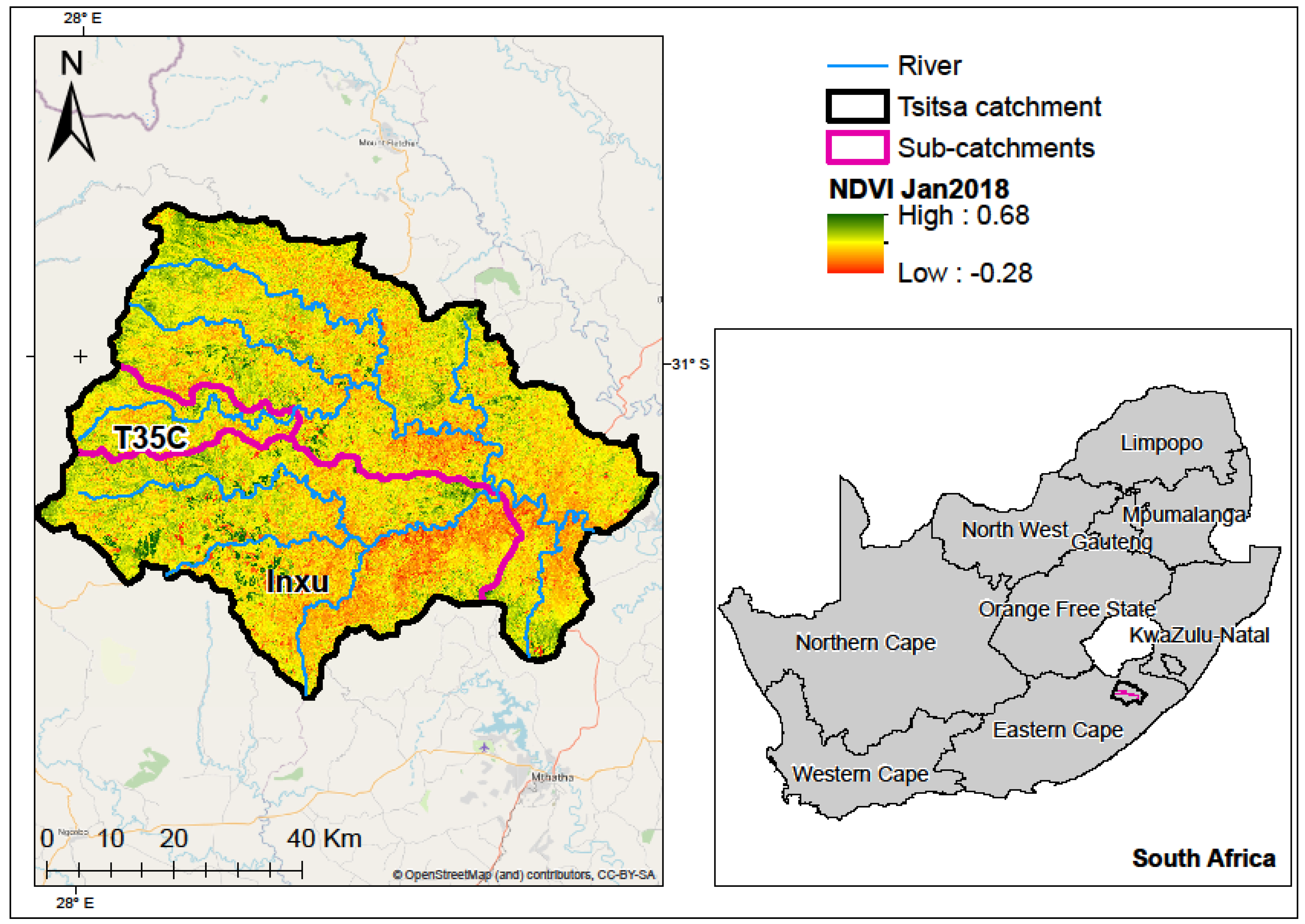
The Tsitsa River catchment is part of the larger Umzimvubu River catchment and the Eastern Cape Province of South Africa (Figure 1). The Tsitsa River Catchment lies in a mountainous region characterised by steep mountain slopes, gentle undulating foot slopes, and almost flat valley floors [41]. The complex topography varies considerably in elevation (900–2500 masl).
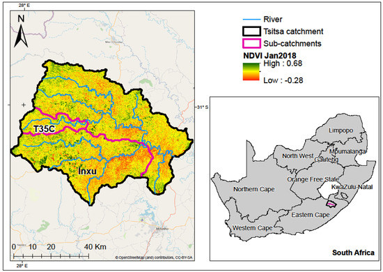
Figure 1.
Map showing the location of the study area in the Eastern Cape Province, South Africa. The Inxu and T35C sub-catchments flow into the greater Tsitsa catchment. The two sub-catchments were modelled independently and as part of the entire catchment.
The catchment is also geologically variable, with high areas around the escarpment consisting of basaltic lava from the Drakensberg formation (Jurassic), underlain by a stratum of Triassic sandstones and mudstones [41]. The most frequent geological formation is the fine sandstones from the Clarens formation, followed by mudstones from the Elliot formation and sandstones of the Molteno formation [41]. There is also a small presence of quaternary alluvium and intrusive dolerites occurring in thin bands.
Soil depth is relatively low on the steep slopes and gradually deepens towards the foot slopes and valley bottom areas due to colluvial and alluvial deposits. The thin soils on steeper slopes become highly erodible when vegetation is removed [42], and this situation is exacerbated by livestock over-grazing. Highly erodible duplex soils occur in some parts of the catchment, resulting in massive gullying [43].
The climate is characterised by a distinct seasonality in rainfall and temperature. Most rainfall (around 80%) occurs during the summer (October to March), whereas winters are generally dry [44]. Mean annual rainfall ranges from 625 mm in the low-lying areas to 1415 mm in the mountainous regions [44]. Mean monthly temperatures range from 7 °C in winter to 19 °C in summer, with high variation during the day.
The Tsitsa River catchment is dominated by the grassland biome, whereas the Eastern valley bushveld thrives along river channels in the lower catchment [45]. The natural vegetation is primarily influenced by altitude and burning [41], and small pockets of the Afromontane forest occur along drainage lines and ravines, where fire has a minimal effect. The National Land Cover [46] database shows that over 60% of the catchment area is covered by grassland. Patches of natural forest also occur alongside forest plantations. Other minority land cover/uses include commercial and subsistence agriculture, water bodies, bare/degraded land, and urban and rural settlements [46].
2.2. Acquiring and Processing NDVI Data
Mean monthly (years 2016–2017) values of catchment NDVI were accessed from Google Earth Engine (GEE) [47] based on a script made available by the GEE developers (https://code.earthengine.google.com/, accessed on 1 July 2020). LAI was also accessed from GEE in order to assess the relationship between LAI and NDVI in the catchment. For spatially distributed NDVI data, it was necessary to download and process images within ArcGIS (ESRI, Redlands, CA, USA) to extract spatial attributes. Therefore, ‘Landsat 8 OLI/TIRS C-1 Level-2’ images were acquired. The data are atmospherically corrected surface reflectance values. The raw satellite imagery used within the present study is freely downloadable from the United States Geological Survey (USGS) Earth Explorer (https://earthexplorer.usgs.gov/, accessed on 1 February 2018).
The imagery acquired were less contaminated with cloud cover because images with >10% cloud cover were filtered in the search criteria. Two approaches were used to assess the impacts of a variable C factor. The first was an inter-annual analysis over six years starting in 2013 (the launch year of the satellite) and based on data for a single month (see Table 1). Satellite images from March were chosen at the suggestion of [8] that a single image selected over the main erosive season can suffice to describe the annual variability in the C factor. March is part of the summer rainfall season and images for that month had the least cloud cover. The second approach represents an intra-annual analysis using data for all months over two years, 2016–2017.

Table 1.
Dates of images acquired for inter-annual analysis.
For the downloaded satellite images, the red (band 4) and near-infrared (band 5) data of Landsat 8 images were used in the analysis. NDVI was computed from these band images using the ‘Raster calculator’ tool in ArcGIS 10.3. The expression used for calculating the NDVI is:
2.3. NDVI to C Factor Conversion
Several methods of scaling NDVI to the C factor were assessed in order to find a method that could be applied to the present study area. The assessment revealed that some methods calculated C values that were outside the 0–1 from NDVI values above certain thresholds (e.g., [31,48,49]) (see Table S1). Other methods calculated C factors that were too high [11]. The method proposed by [32] gave C factor values within the reasonable range without the need for modification (Equation (2)); hence, it was adopted for use in the current study:
In Equation (2), α and β are parameters that determine the shape of the NDVI—C factor curve, with values of 2 and 1, respectively. A low NDVI suggests little or no vegetation and results in a high C factor, while a high NDVI results in a lower C factor.
The method proposed by [32] has been criticised for underestimating the C factor in areas with intense rainfall [48], with specific reference to a catchment in Brazil. However, a recent study by [4] reported that the same method over-estimates the C factor in a tropical Brazilian catchment. Such disparities highlight the uncertainties associated with the method, so that it is vital to assess if predicted C factor values correspond with field-collected data [49]. In the current study, an assessment of the predicted C factor was performed by collecting GPS points for each land cover (up to five replicates); more than ten replicates for the prominent grass-cover type and then comparing the C factor of each cover type to the NDVI-calculated C factor for the same area. The comparison yielded linear regression R2 = 0.75 compared to field data (see Table S2), indicating that the calculated NDVI C was a good predictor of the literature-suggested C values for the specific land-cover types. A similar assessment was used by [31] and [32].
Differences in the intra-annual variations in the C factor were also analysed for the two most prominent natural vegetation cover classes: grass (74%) and thicket/forest (5%). This analysis was designed to assess which vegetation class was more variable, and thus might have a significant influence on the mean catchment C. Vegetation classes (e.g., cultivation [1.4%] and plantations [14.8%]) were not included because their temporal variation may depend on human influence and the management information with regards to planting and cropping is not easily accessible.
2.4. Sediment Yield Calculations
Three catchments, including the main Tsitsa catchment and sub-catchments Inxu and T35C, were considered for the analysis and were all modelled independently. Initially, the smaller T35C was used for the long-term inter-annual and two-year intra-annual analysis. The other two catchments subsequently served to validate the outcome of the T35C analysis based on observed sediment data. The sediment yield calculations were conducted using the MUSLE, as applied in [50,51] in the form:
where Sy is sediment yield (tons ha−1) for the entire catchment, is runoff depth in mm, qdp is peak runoff in mm h−1, and Area is the total catchment area in ha. K, LS, C and P are the soil erodibility, slope length and steepness, cover management, and soil erosion control practice factors, respectively. The MUSLE factors were calculated similarly to [51] from readily available spatial and hydrological datasets. Discharge data for the greater Tsitsa and T35C catchments were accessed from the Department of Water and Sanitation (DWS; http://www.dwa.gov.za/Hydrology/Verified/hymain.aspx, last accessed 20 August 2020). Observed sediment data and discharge for the Inxu and Tsitsa catchments were measured under the Tsitsa Project (see [51,52]),but only a few months of daily observed data were available in both catchments. Seven months of data were available for the Inxu (October 2016 to April 2017). Monthly data were available for the Tsitsa catchment in 2016, except for October. The LS factor was calculated from the Shuttle Radar Topography Mission (SRTM) 30 m DEM (https://earthexplorer.usgs.gov/ last accessed 1 February 2020) and ArcGIS 10.3.1. Soil erodibility data were obtained from the South African Atlas of Climatology and Agro hydrology database [53]. The fixed C and P factors were estimated from the South African National Land Cover [46] database (https://www.sanbi.org/biodiversity/foundations/national-vegetation-map/ last accessed 21 July 2016), whereas the NDVI C factor was calculated as explained in the previous section. Tables with the calculated MUSLE factors are presented in Table S3.
The focus of the application was to assess whether the potential temporal variability in the C factor would lead to significant differences in cumulative sediment yield. To achieve this, the model was first run with fixed C factor inputs calculated using the widely used land-cover/use maps and, secondly, run with variable C factor inputs calculated using the NDVI method (Section 2.3). Although the model was applied at a daily timescale, computed monthly C factors remained constant over the entire month and the entire year for the intra-annual and inter-annual analyses, respectively. The fixed C factor remained constant across all the timescales. The flow data input to the model was based on records of observed daily discharge. Sediment outputs were evaluated based on the R2, PBIAS [54] and Nash Sutcliffe Efficiency (NSE) [55].
3. Results
3.1. Fixed C Factor
The fixed C factor for catchment T35C was calculated as 0.098. Table 2 summarises the C factor calculation for the T35C catchment using land-cover/use maps and C values from the literature. The total weighted C factor was used as the C factor value within the MUSLE.
Table 2.
Fixed catchment (T35C) C factor calculated using maps and values from the literature.
3.2. NDVI and Variable C Factors
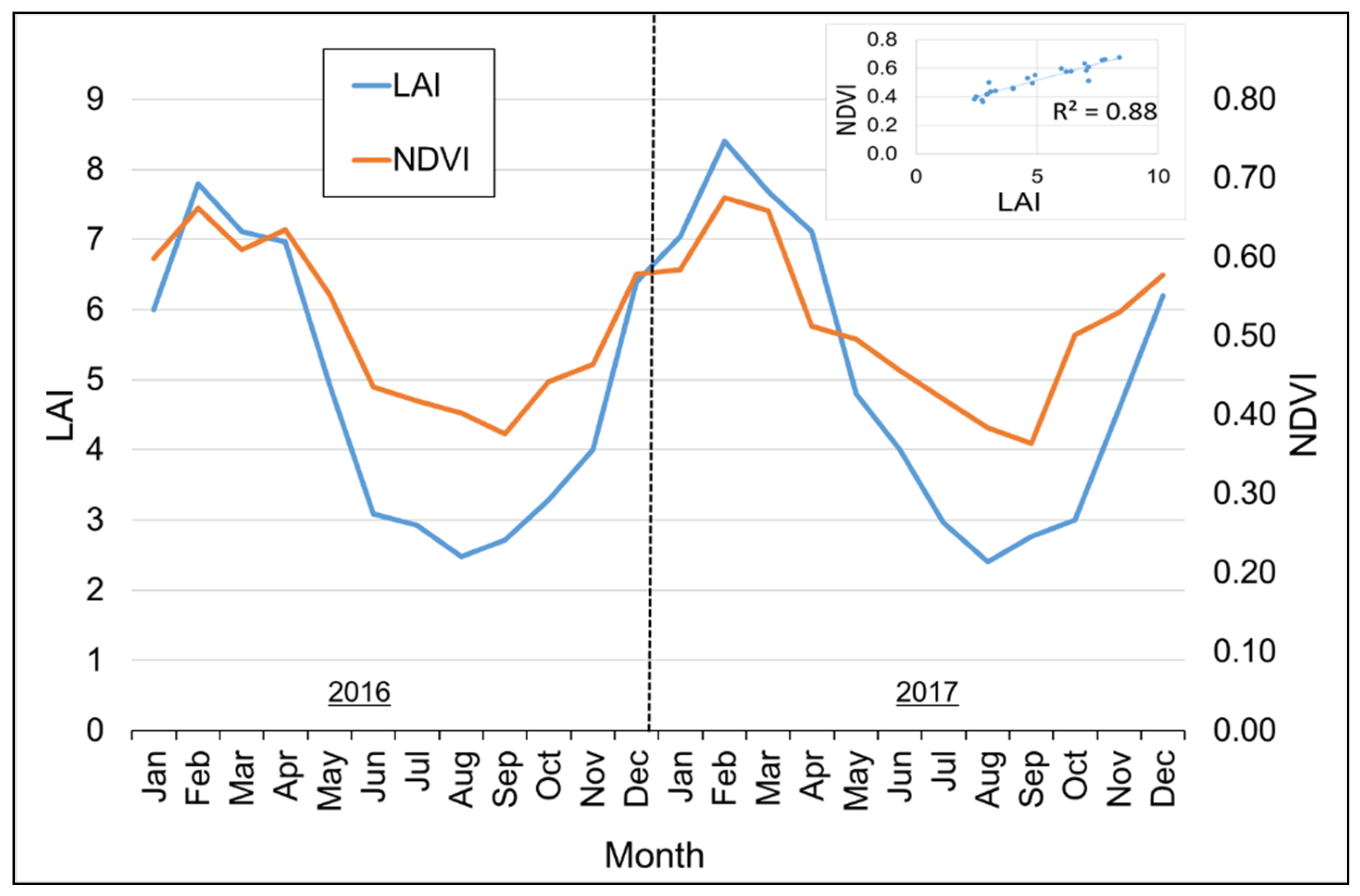
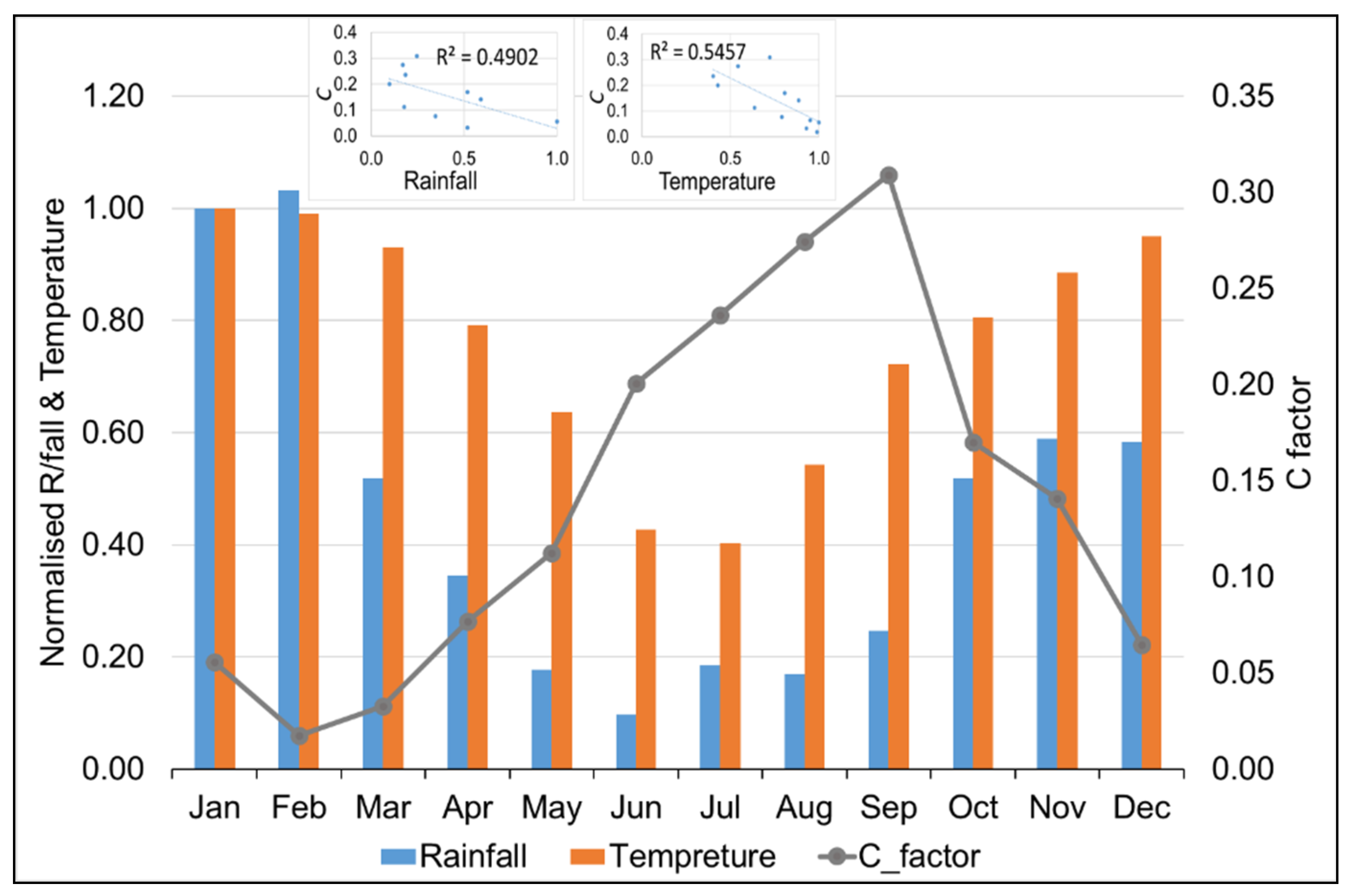
Figure 2 illustrates that the NDVI values are higher for the summer rainfall months and lower during the generally drier and cold winter months. They generally start to increase with the onset of the rainfall season after September. Figure 3 indicates a weak positive linear relationship (R2 = 0.49) between NDVI/C factor and rainfall and a somewhat stronger linear relationship (R2 = 0.55) with temperature. A similar trend in the monthly NDVI was noted for 2017 (Figure 2). The lowest C values occurred in February during both years (0.02 in 2016 and 0.016 in 2017), while the highest values of 0.30 and 0.32 were obtained in September for 2016 and 2017, respectively. The LAI displays a similar seasonal trend compared to the NDVI; a strong linear regression (R2 = 0.88) is exhibited between the LAI and NDVI (Figure 2). LAI is shown to be much higher in the mid-summer season (Jan–Mar), when leaf development is at its peak.
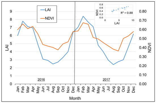
Figure 2.
Distribution of monthly NDVI and LAI factor for 2016–2017.

Figure 3.
The relationship between normalised rainfall and temperature with C factor; insert linear regression of rainfall, temperature and C factor for 2016–2017. The climate values were normalised by dividing all values by the first value in the distribution (i.e., January).
The inter-annual C factor distribution presented in Table 3 shows the differences between the variable C factor (based on March NDVI data) and the fixed value. It is immediately apparent that C factors calculated for March are much lower than the fixed values calculated from the literature values of vegetation-cover types. Figure 3 illustrates that the late autumn to early spring (May to September) C values are much higher than the fixed C value or the single-month NDVI estimate. However, as already noted, the important issue regarding impacts on sediment yield depends on the seasonal variations in the erosivity factor driven by the runoff data.
Table 3.
Percentage variation between inter-annual (based on March values) and fixed C factors for catchment T35C.
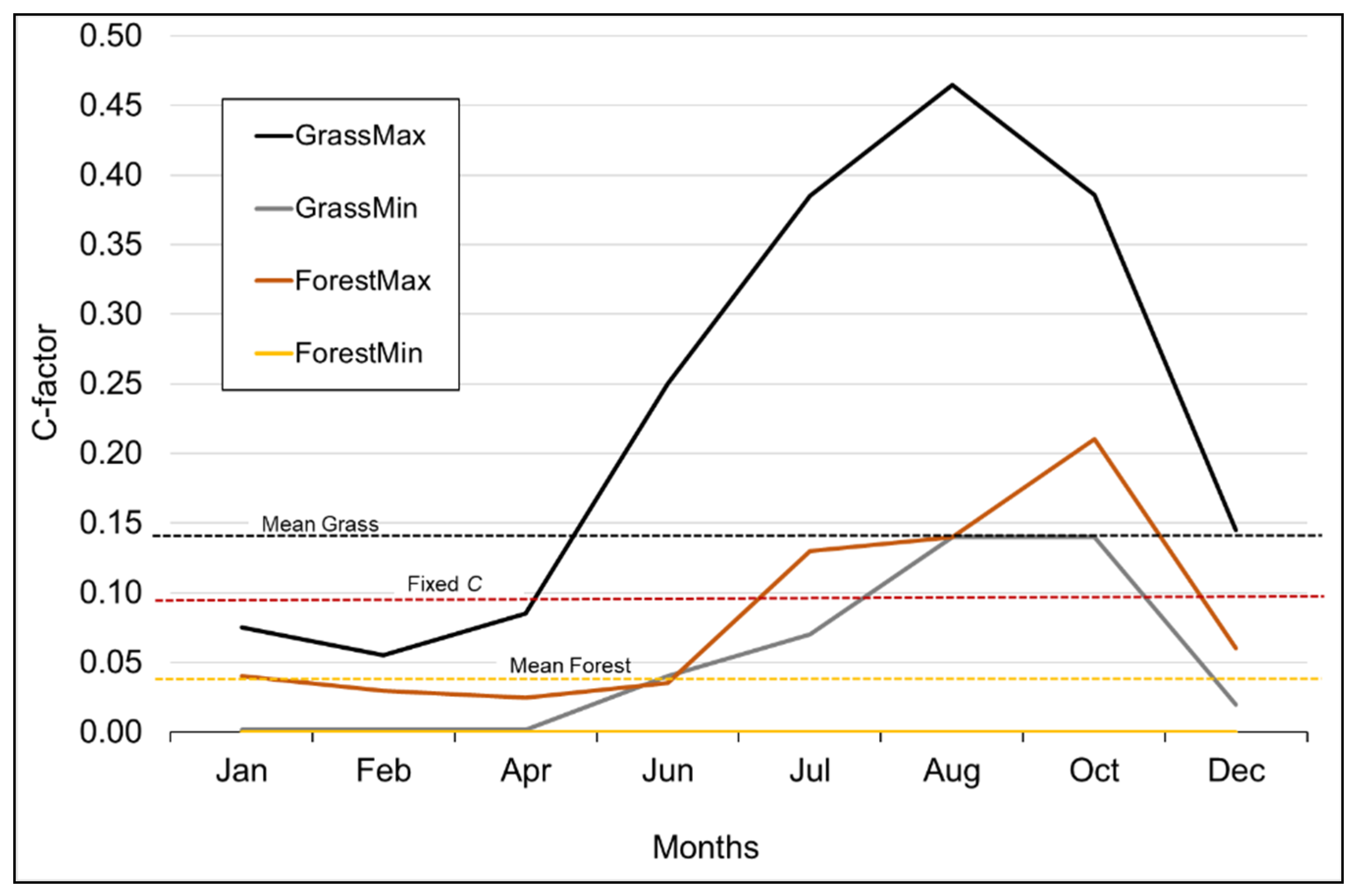
Figure 4 illustrates the variation in the C factor values derived from NDVI data for the two main vegetation types within the T35C catchment. The maximum and minimum values represent the range of calculated NDVI C values across all the pixels classified into the two vegetation types. The grassland type has the largest seasonal range, particularly in the maximum values and the largest difference between maximum and minimum values. This could reflect the fact that grasslands in this area include both natural grassland and heavily grazed and, therefore, degraded grassland. The minimum values for the thicket/dense bush vegetation type are always 0, while the maximum values vary from 0.04 in the wet season to 0.21 in the dry season. This may reflect the variations in the location of the bush areas within the landscape, with the consistently low values lying in well-watered valley bottom locations, while the more variable C values reflecting locations on slopes and ridges that are more prone to seasonal variations in moisture availability.
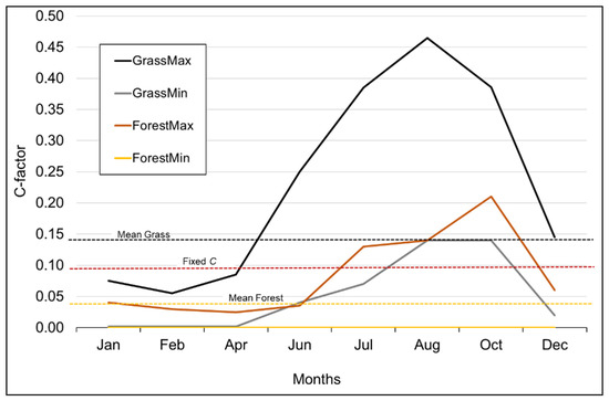
Figure 4.
Monthly C factor distribution of the grass and forest vegetation classes in the T35C catchment for the year 2016 calculated from NDVI.
3.3. T35C Catchment Sediment Yield (SY) Distribution
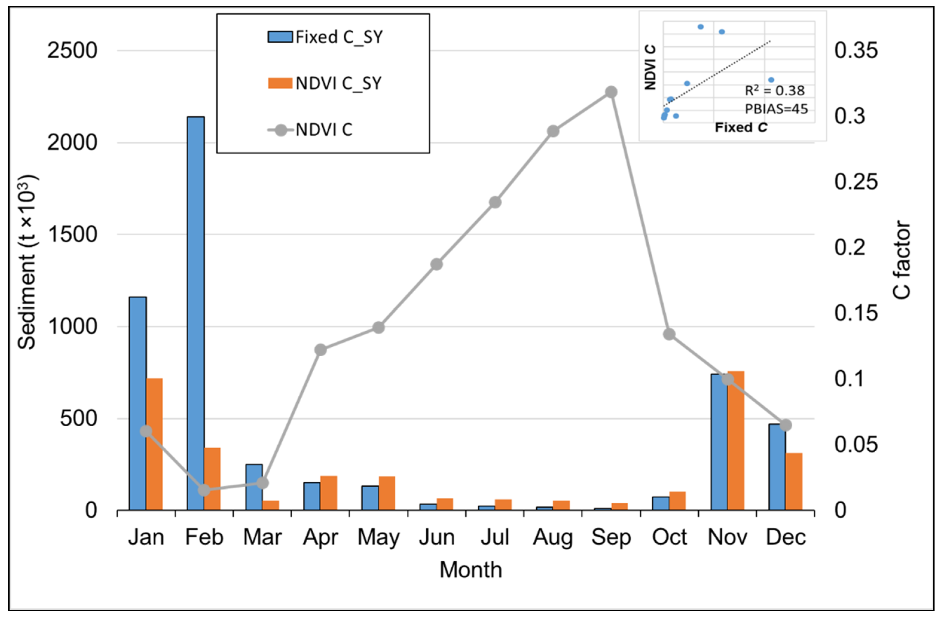
The results for 2016 (Figure 5) show that the fixed C factor yielded much higher sediment output than the variable C factor, with total annual sediment yields calculated as 5464 × 103 and 4625 × 103 tons, respectively. The major differences occur in the three main summer runoff months. These impacts are somewhat offset by higher sediment yields using the variable C factor in the winter and spring months when the C values are quite substantially higher than the fixed value. The results for 2017 (Figure 6) also display the typical seasonal variability exhibited in 2016. However, there is a larger difference between the total sediment yields simulated using the fixed (5203 × 103 tons) and dynamic (2871 × 103 tons) C factors. In 2017, the sediment generated during the two main summer months (January and February) is substantially reduced. There is little sediment generated during the winter. During November and December, the fixed and variable C values are similar. The analyses of the two years indicate that the differences between the use of fixed and variable C factor values are dependent upon the rainfall and streamflow regime during the year and whether the dominant erosion and transport events occur during the year when the variable values are close to, or very different from, the fixed estimates.
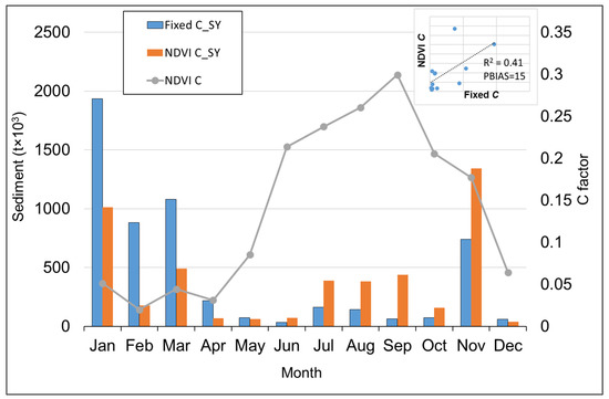
Figure 5.
Distribution of sediment yield (SY) simulated using the fixed and variable (NDVI) C factors for catchment T35C in 2016.
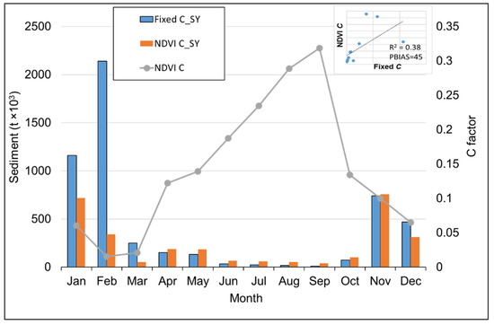
Figure 6.
Distribution of sediment yield (SY) simulated using the fixed and variable (NDVI) C factors for catchment T35C in 2017.
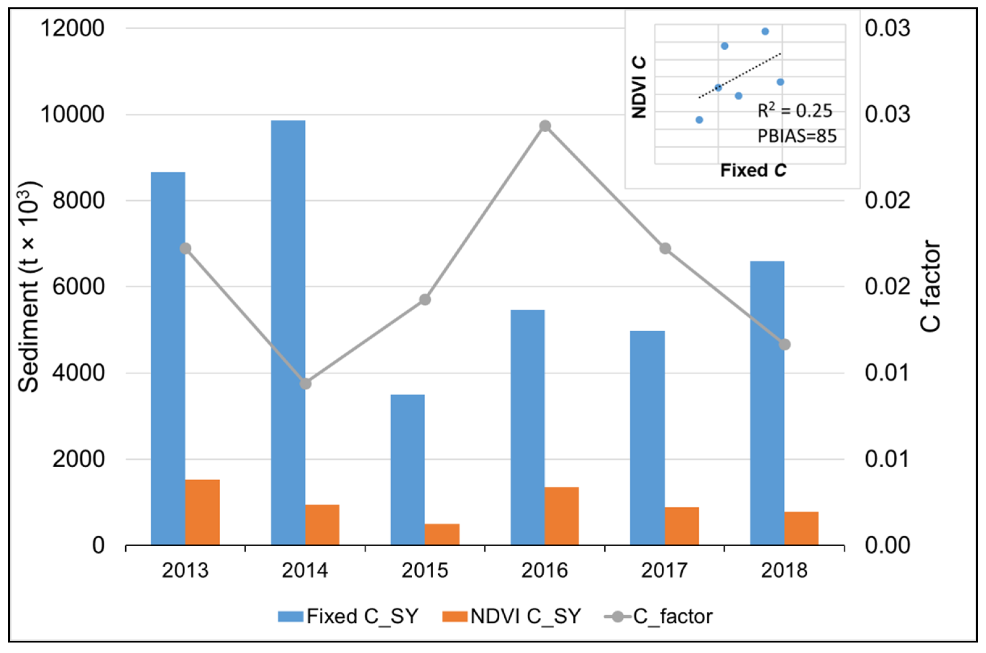
Figure 7 shows the results of the inter-annual analysis using annual variations in the C factor based on March NDVI data, compared with a fixed C value. The differences are substantially greater than those revealed by the intra-annual analysis based on 2016 and 2017. The variable C value results in approximately 85% less sediment compared to 16% and 45% less based on the intra-annual analysis for 2016 and 2017. This is a result that could have been predicted from the data provided in Table 3, which indicates that the March-based C values are only ~15% of the fixed value. The clear conclusion is that using a single month to determine the annual variability in C values is likely to be a very uncertain exercise.
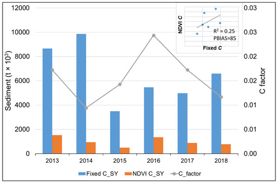
Figure 7.
Sediment yield (SY) variation resulting from the fixed and variable (NDVI) C factor.
3.4. Validating the C Factor Assessment in the Tsitsa Catchment and Inxu Sub-Catchment
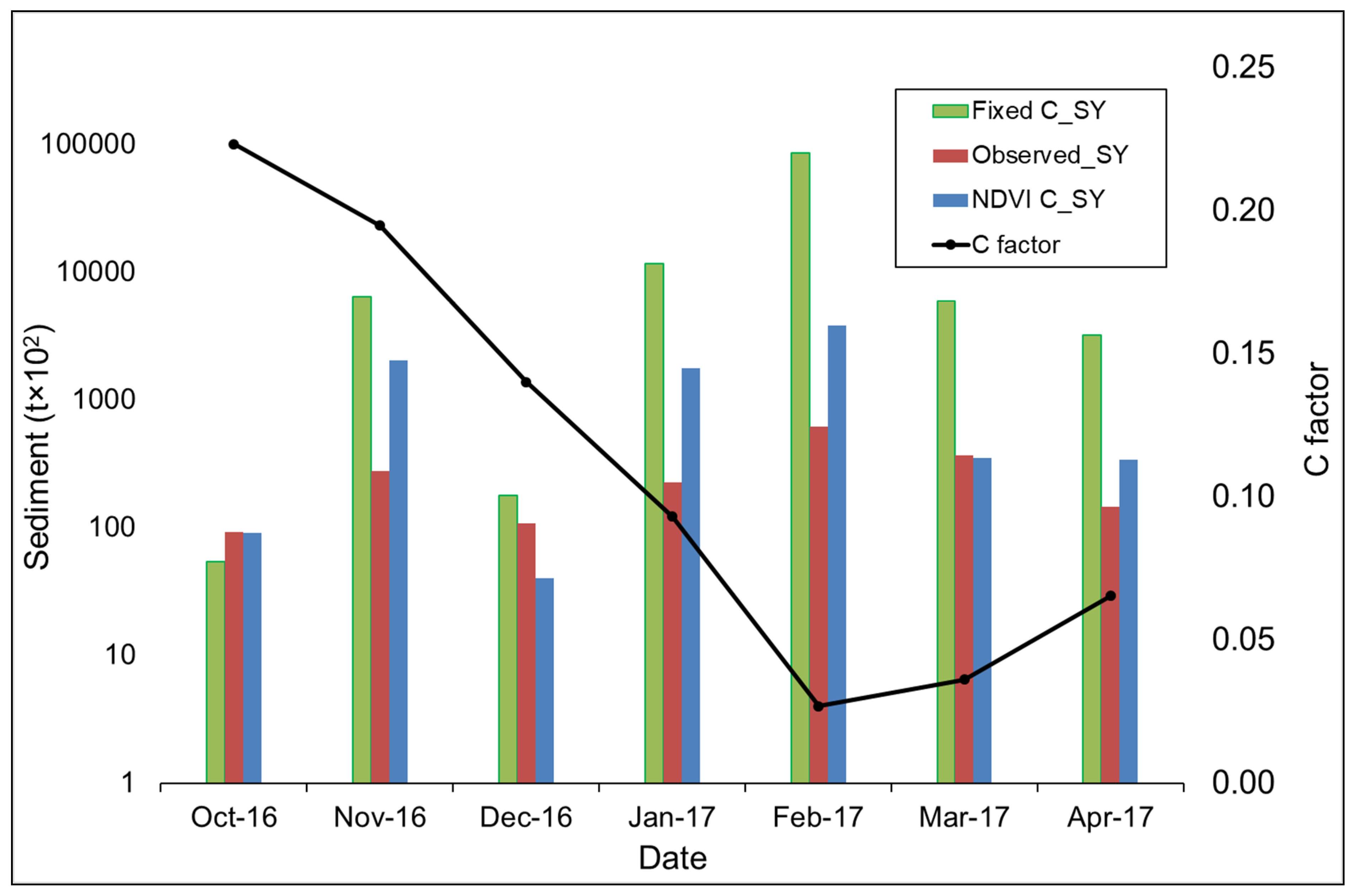
The results summarised in Table 4 and Figure 8 and Figure 9 corroborate the findings reported in Section 3.3, showing that using a fixed C factor results in the over-estimation (up to ten times higher) of sediment yield compared to observed data in both sample catchments. However, the R2 values for both daily and monthly time scales suggest that the poor results are a consequence of systematic bias. Given that the C factor is a linear multiplier in the MUSLE, it could be calibrated (together with the other linear factors in the equation) to generate a much more acceptable result based on the NSE and PBIAS statistics. This would involve reducing the fixed C value. For the Inxu, the use of a variable C factor leads to an under-estimation of about 80% but a much higher over-estimation exists when the fixed C is applied. While the NSE and PBIAS statistics are much improved (Table 5), the R2 values for daily and monthly are much lower compared with the fixed C factor result. The conclusion is that the fixed C model result is better (in terms of the R2) and that a simple scaling calibration would be effective. For the Tsitsa, the variable factor model results in over-estimation (but less than with a fixed factor), and the conclusions on further calibration are the same as for the Inxu catchment.
Table 4.
Summary of sediment yield (SY) output in the Inxu and Tsitsa catchments compared to observed data.
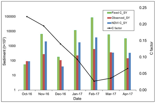
Figure 8.
An illustration of observed sediment yield (SY) versus sediment calculated using the fixed and variable (NDVI) C factors in the Inxu catchment (Log Y-axis).
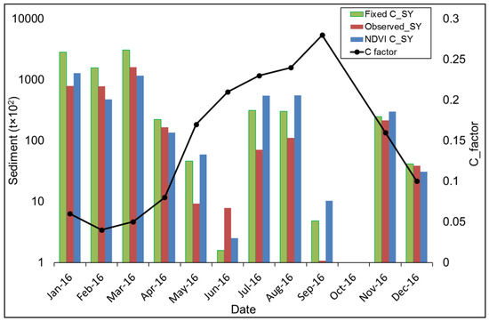
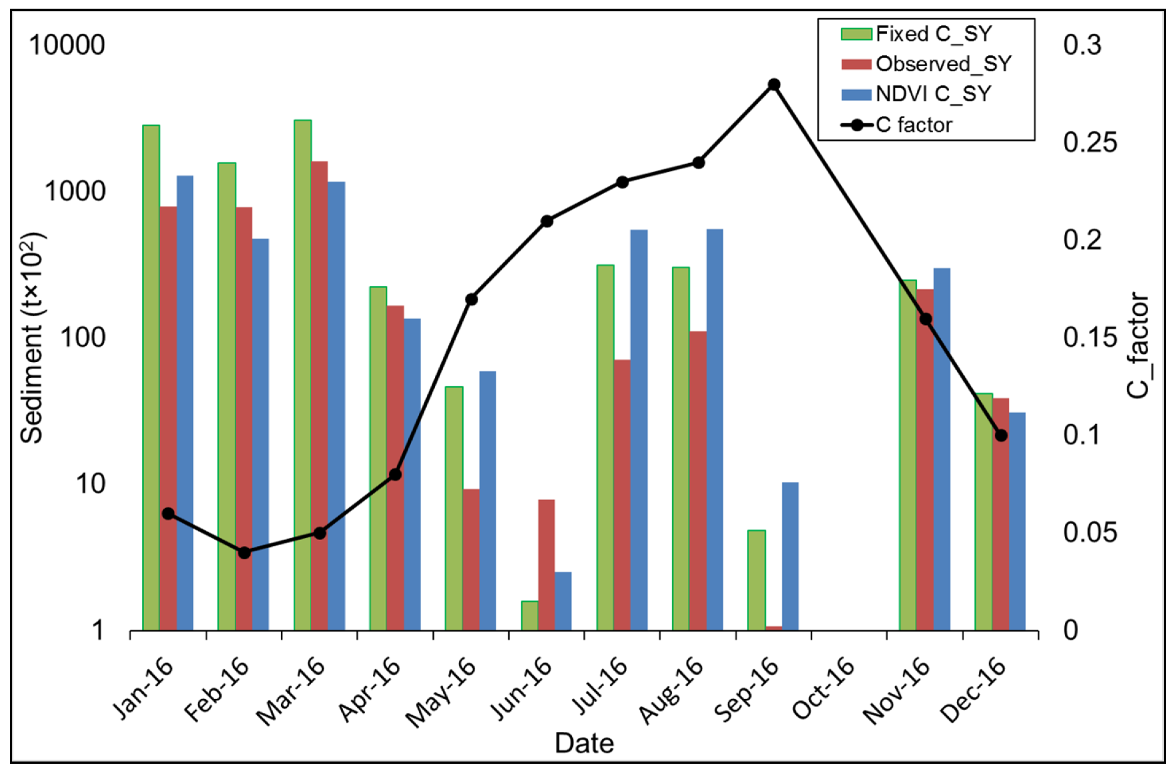
Figure 9.
An illustration of observed sediment yield (SY) versus sediment calculated using the fixed and variable (NDVI) C factors in the Tsitsa catchment (Log Y-axis).
Table 5.
Summary statistics comparing observed data sediment yield (SY) output attained using a fixed or variable C factor at daily and monthly timescales.
The limited observed records available for the Inxu catchment preclude an analysis of the seasonal variations in sediment output. However, the relatively short record for the Tsitsa suggests that winter runoff and sediment yield can play a quite important role, at least in some years. Therefore, it is interesting to note that the largest over-simulations occur from the late autumn to early summer months, when the estimated C values are quite high. This could reflect the uncertainties in the use of the NDVI data to estimate the C values, particularly when the NDVI values are low in winter when the organic matter cover on the soil surface still provides some protection from erosion.
4. Discussions and Conclusions
In general, the analysis showed greater intra-annual variability in the C factor as compared to inter-annual variability. The findings of [8] support the above result, as they found that vegetation cover and, hence, the C factor, can show high intra-year variability, depending on seasonal effects and land management. A correlation of C factor values between the months of years 2016 and 2017 yielded 0.9, indicating that there was little variability in the distribution of C factor values on a month-to-month basis for the two years.
The linear regressions between the C factor, temperature, and rainfall (Figure 3) show no strong individual linear relationships between rainfall or temperature and the C factor derived from NDVI, although the relationship with temperature is slightly higher. This can partly be attributed to the fact that both temperature and moisture availability are likely to affect increased NDVI values [56], and that vegetation cover response to rainfall and temperature is likely to be lagged. The strong linear relationship between LAI and NDVI (Figure 2) in the catchment is important [37], as both have been criticised [6] for different reasons: NDVI for failure to represent the erosion resistance of poor vitality vegetation as it is bound to chlorophyll reflectance, and LAI for failure to represent short stature vegetation (e.g., grasses).
Additional criticism concerning the failure of both LAI and NDVI to represent poor vitality and above-ground biomass of short-stature vegetation (during winter) reveals a major shortcoming of the two spectral indices. This limitation is apparent in the Tsitsa catchment results, where overestimates in winter dominated the simulations, while many of the overestimates for the short Inxu data record are in spring and early summer, before the NDVI values reach their highest peaks. Accordingly, the popular methods of calculating the integrated C factor at the plot scale then extrapolating/scaling the information to larger areas using land-use/land cover areas (e.g., [14]) have already been identified as flawed by [57]. Both the Inxu and Tsitsa examples highlight the likely over-simulations that might occur by using a fixed C factor based on land cover and look-up tables. While the use of the NDVI-derived variable C values improved the simulations, substantial uncertainties remain in the applicability of the NDVI-based estimation methods for the C factor. The developers of the NDVI to C factor conversion methods did not seem unaware of the limitations of the index but sought to conduct a direct conversion based on the similarity of the range of NDVI values to the original C factor range.
The present study results suggest that failure to account for temporal changes in vegetation cover may add to some of the many uncertainties associated with modelling sediment yield. The sediment yield simulations using the fixed C factor were generally higher because the wet summer season C values are typically lower than the fixed value. The fact that a high C factor might not translate into high sediment yield if there is limited runoff during the winter season is a somewhat obvious conclusion. However, the admittedly short period of data for the Tsitsa catchment suggests that winter rainfall and runoff is possible in at least some years and locations in this region and climate type of South Africa. This implies that the apparent overestimation of the C factor in winter could be important and represents a major limitation of the NDVI estimation approach. It is also evident from both catchments that the transition months from low to high C values (autumn), and from high to low values (spring) can represent periods when sediment load over-estimations occur. The overall conclusion is that while the NDVI approach is useful in terms of identifying spatial and temporal variations in the C value, the actual estimation equation (Equation (1)) requires some revisions. Revisions may also focus on the method of NDVI calculation, as proposed by [5]. It is likely that these revisions may be site-specific. For example, the effects of using the approach in the winter rainfall regions of the Western Cape Province may be quite different from the effects illustrated in the T35 region of the Eastern Cape (mainly summer rainfall, but with some winter rainfall), and may be different again in other parts of South Africa where winter rainfall is sporadic. The inter-annual analysis, based on annual variations using a fixed month, illustrated that this somewhat simpler approach to allowing for C variations will be very uncertain. This is particularly true for a region with a variable rainfall (and therefore runoff) regime in which high rainfall events can occur during most months of the year, even if they are more frequent during the summer months.
The analysis of C variability across the two vegetation types (Figure 4) suggests that any revisions to the NDVI-based estimation approach may also need to be vegetation-type specific. The seasonal and spatial variations in the derived C values are much greater for the dominant grassland type than for the less frequent bush/forest type. This has a substantial impact on sediment yield variations, as the grass has the highest spatial coverage in all the catchments. A further potentially related issue is that over-grazing has often been cited as one of the reasons for high sediment loads in the T35 region [43,58]. However, it is also suggested that a great deal of the sediment load may be derived from gully erosion [43], which is not explicitly simulated by the MUSLE and, therefore, is a potentially different issue, unrelated to how the seasonal C values are estimated.
The availability of satellite data and GIS processing tools allows for an alternative approach to the use of a lumped C factor estimation using land-cover maps by employing spatially distributed approaches based on spectral indices such as NDVI. Nevertheless, access to high-quality satellite data is often expensive, and some available data may not be useful for analysis because of problems such as poor resolution and cloud cover. Although cloud cover removal techniques are available, this only adds uncertainty to the quality of the pre-processed image. Consequently, some of the 30 m Landsat data used were carefully selected and manually processed to ensure the quality of the NDVI output. However, as the analysis was conducted in a single region over a small number of years, more robust assessments are needed to investigate the NDVI-to-C-factor conversion used in this initial assessment. Nevertheless, the study highlights the variations in outputs associated with different approaches to estimating the C factor. Increasing spatial and temporal resolution is vital for describing catchment processes in greater detail. Maintaining simplicity in model parameterisation is also important in data-scarce regions and the results should assist potential users in anticipating the likely effects of scale (temporal and spatial) in MUSLE applications. Overall, the current study shows the importance of adopting a monthly/seasonal distribution of C factor values when applying the MUSLE to calculate sediment and highlights several uncertainties in the current methods used to calculate the variability of the C factor.
Supplementary Materials
The following are available online at https://www.mdpi.com/article/10.3390/w13192707/s1, Table S1: Assessing NDVI C against control points collected in the field, Table S2: The performance of some of the NDVI to C conversion methods for use within the study area, Table S3: Average MUSLE factors (including fixed C) calculated for the catchments.
Author Contributions
D.G., D.A.H., A.R.S. and S.K.M. conceived and designed the study; D.G. undertook modelling and data analysis under the guidance of D.A.H., A.R.S. and S.K.M.; D.G. wrote the paper with support from D.A.H., A.R.S. and S.K.M. All authors have read and agreed to the published version of the manuscript.
Funding
The project has been supported by the Water Research Commission of South Africa under project K5/2448.
Institutional Review Board Statement
Not applicable.
Informed Consent Statement
Not applicable.
Data Availability Statement
The datasets in this study are freely available global and regional datasets. Other datasets can be availed upon request.
Acknowledgments
We are grateful that part of the project has been supported by the Water Research Commission of South Africa under project K5/2448, which also provided partial support for the post-graduate bursary for the first author. Additional post-graduate financial support was provided by the Carnegie Corporation of New York under the Regional Initiative for Science Education (RISE) programme and the Oppenheimer Memorial Trust (OMT REF 21256/01). We would also like to thank Namso Nyamela and Laura Bannatyne for providing observed sediment data for the Tsitsa and Inxu catchments.
Conflicts of Interest
The authors declare no conflict of interest.
References
- Langbein, W.B.; Schumm, S.A. Yield of sediment in relation to mean annual precipitation. Trans. Am. Geophys. Union 1958, 39, 1076–1084. [Google Scholar] [CrossRef] [Green Version]
- Moglen, G.E.; Eltahir, E.A.B.; Bras, R.L. On the sensitivity of drainage density to climate change. Water Resour. Res. 1998, 34, 855–862. [Google Scholar] [CrossRef] [Green Version]
- Wischmeier, W.H.; Smith, D.D. Predicting rainfall erosion losses. Agric. Handb. 1978, 537, 285–291. [Google Scholar] [CrossRef]
- Almagro, A.; Thomé, T.C.; Colman, C.B.; Pereira, R.B.; Junior, J.M.; Rodrigues, D.B.B.; Oliveira, P.T.S. Improving cover and management factor (C-factor) estimation using remote sensing approaches for tropical regions. Int. Soil Water Conserv. Res. 2019, 7, 325–334. [Google Scholar] [CrossRef]
- Macedo, P.M.S.; Oliveira, P.T.S.; Antunes, M.A.H.; Durigon, V.L.; Fidalgo, E.C.C.; de Carvalho, D.F. New approach for obtaining the C-factor of RUSLE considering the seasonal effect of rainfalls on vegetation cover. Int. Soil Water Conserv. Res. 2021, 9, 207–216. [Google Scholar] [CrossRef]
- Schmidt, S.; Alewell, C.; Meusburger, K. Mapping spatio-temporal dynamics of the cover and management factor (C-factor) for grasslands in Switzerland. Remote Sens. Environ. 2018, 211, 89–104. [Google Scholar] [CrossRef]
- Renard, K.; Foster, G.; Weesies, G.; McCool, D.; Yoder, D. Predicting Soil Erosion by Water: A Guide to Conservation Planning with the Revised Universal Soil Loss Equation (RUSLE). Agricultural Handbook No. 703. 1997; pp. 65–100. Available online: https://www.ars.usda.gov/arsuserfiles/64080530/rusle/ah_703.pdf (accessed on 1 June 2016).
- Vrieling, A.; De Jong, S.; Sterk, G.; Rodrigues, S.C. Timing of erosion and satellite data: A multi-resolution approach to soil erosion risk mapping. Int. J. Appl. Earth Obs. Geoinf. 2008, 10, 267–281. [Google Scholar] [CrossRef]
- Williams, J.R. Sediment yield prediction with universal equation using runoff energy factor. In Present and Prospective Technology for Predicting Sediment Yield and Sources; USDA-ARS: Washington, DC, USA, 1975; Volume 40, pp. 244–254. [Google Scholar]
- Smith, S.J.; Williams, J.R.; Menzel, R.G.; Coleman, G.A. Prediction of sediment yield from southern plains grasslands with the modified universal soil loss equation. J. Range Manag. 1984, 37, 295. [Google Scholar] [CrossRef]
- Sulistyo, B. The effect of choosing three different C factor formulae derived from NDVI on a fully raster-based erosion modelling. IOP Conf. Ser. Earth Environ. Sci. 2016, 47, 012030. [Google Scholar] [CrossRef] [Green Version]
- Karydas, C.; Panagos, P.; Gitas, I. A classification of water erosion models according to their geospatial characteristics. Int. J. Digit. Earth 2012, 7, 229–250. [Google Scholar] [CrossRef]
- Alewell, C.; Borrelli, P.; Meusburger, K.; Panagos, P. Using the USLE: Chances, challenges and limitations of soil erosion modelling. Int. Soil Water Conserv. Res. 2019, 7, 203–225. [Google Scholar] [CrossRef]
- Colman, C.; Oliveira, P.; Almagro, A.; Soares-Filho, B.; Rodrigues, D. Effects of climate and land-cover changes on soil erosion in Brazilian pantanal. Sustainability 2019, 11, 7053. [Google Scholar] [CrossRef] [Green Version]
- Arekhi, S.; Shabani, A.; Rostamizad, G. Application of the modified universal soil loss equation (MUSLE) in prediction of sediment yield (case study: Kengir Watershed, Iran). Arab. J. Geosci. 2011, 5, 1259–1267. [Google Scholar] [CrossRef]
- Noor, H.; Mirnia, S.K.; Fazli, S.; Raisi, M.B.; Vafakhah, M. Application of MUSLE for the prediction of phosphorus losses. Water Sci. Technol. 2010, 62, 809–815. [Google Scholar] [CrossRef] [PubMed]
- Pan, J.; Wen, Y. Estimation of soil erosion using rusle in Caijiamiao watershed, China. Nat. Hazards 2014, 71, 2187–2205. [Google Scholar] [CrossRef]
- Sadeghi, S.; Gholami, L.; Darvishan, A.K.; Saeidi, P. A review of the application of the MUSLE model worldwide. Hydrol. Sci. J. 2014, 59, 365–375. [Google Scholar] [CrossRef] [Green Version]
- Sepuru, T.K.; Dube, T. An appraisal on the progress of remote sensing applications in soil erosion mapping and monitoring. Remote Sens. Appl. Soc. Environ. 2018, 9, 1–9. [Google Scholar] [CrossRef]
- De Asis, A.M.; Omasa, K. Estimation of vegetation parameter for modeling soil erosion using linear spectral mixture analysis of landsat ETM data. ISPRS J. Photogramm. Remote Sens. 2007, 62, 309–324. [Google Scholar] [CrossRef]
- Wang, G.; Wente, S.; Gertner, G.Z.; Anderson, A. Improvement in mapping vegetation cover factor for the universal soil loss equation by geostatistical methods with Landsat Thematic Mapper images. Int. J. Remote Sens. 2002, 23, 3649–3667. [Google Scholar] [CrossRef]
- Phinzi, K.; Ngetar, N.S.; Ebhuoma, O. Soil erosion risk assessment in the Umzintlava catchment (T32E), Eastern Cape, South Africa, using rusle and random forest algorithm. S. Afr. Geogr. J. 2021, 103, 139–162. [Google Scholar] [CrossRef]
- Rouse, J.W.; Haas, R.H.; Schell, J.A.; Deering, D.W.; Harlan, J.C. Monitoring the Vernal Advancements and Retrogradation of Natural Vegetation; NASA/GSFC: Greenbelt, MD, USA, 1974; pp. 1–137. [Google Scholar]
- Huete, A.R.; Didan, K.; Van Leeuwen, W. Modis vegetation index. Veg. Index Phenol. Lab 1999, 3, 129. [Google Scholar]
- Glenn, E.P.; Huete, A.R.; Nagler, P.L.; Nelson, S.G. Relationship between remotely-sensed vegetation indices, canopy attributes and plant physiological processes: What vegetation indices can and cannot tell us about the landscape. Sensors 2008, 8, 2136–2160. [Google Scholar] [CrossRef] [PubMed] [Green Version]
- Kumari, N.; Srivastava, A.; Dumka, U. A long-term spatiotemporal analysis of vegetation greenness over the Himalayan Region using Google Earth Engine. Climate 2021, 9, 109. [Google Scholar] [CrossRef]
- Pei, F.; Zhou, Y.; Xia, Y. Application of normalized difference vegetation index (NDVI) for the detection of extreme precipitation change. Forests 2021, 12, 594. [Google Scholar] [CrossRef]
- Gandhi, G.M.; Parthiban, S.; Thummalu, N.; Christy, A. Ndvi: Vegetation change detection using remote sensing and gis—a case study of vellore district. Procedia Comput. Sci. 2015, 57, 1199–1210. [Google Scholar] [CrossRef] [Green Version]
- Weier, J.; Herring, D. Measuring Vegetation (NDVI & EVI); NASA Earth Observatory: Washington, DC, USA, 2000. [Google Scholar]
- Cai, C.F.; Ding, S.W.; Shi, Z.H.; Huang, L.; Zhang, G.Y. Study of applying USLE and geographical information system IDRISI to predict soil erosion in small watershed. J. Soil Water Conserv. 2000, 14, 19–24. [Google Scholar]
- De Jong, S.M. Derivation of vegetative variables from a landsat tm image for modelling soil erosion. Earth Surf. Process. Landforms 1994, 19, 165–178. [Google Scholar] [CrossRef]
- Van der Knijff, J.M.; Jones, R.J.A.; Montanarella, L. Soil Erosion Risk Assessment in Italy, Unpublished Report. Ispra: European Commission Directorate General JRC, Joint Research Centre Space Applications Institute European Soil Bureau. 1999. Available online: https://esdac.jrc.ec.europa.eu/ESDB_Archive/serae/GRIMM/italia/eritaly.pdf (accessed on 1 July 2018).
- Alexandridis, T.; Sotiropoulou, A.M.; Bilas, G.; Karapetsas, N.; Silleos, N.G. The effects of seasonality in estimating the C-factor of soil erosion studies. Land Degrad. Dev. 2013, 26, 596–603. [Google Scholar] [CrossRef]
- Bhat, S.A.; Hamid, I.; Rasool, D.; Srinagar, N.; Kashmir, J.; Bashir, I.; Pandit, A.; Khan, S.; Shakeel, C.; Bhat, A.; et al. Soil erosion modeling using rusle & gis on micro watershed of J&K. J. Pharmacogn. Phytochem. JPP 2017, 6, 838–842. [Google Scholar]
- Le Roux, J.; Morgenthal, T.; Malherbe, J.; Pretorius, D.; Sumner, P. Water erosion prediction at a national scale for South Africa. Water SA 2008, 34, 305. [Google Scholar] [CrossRef] [Green Version]
- Sun, W.; Shao, Q.; Liu, J.; Zhai, J. Assessing the effects of land use and topography on soil erosion on the Loess Plateau in China. Catena 2014, 121, 151–163. [Google Scholar] [CrossRef]
- Fan, L.; Gao, Y.; Brück, H.; Bernhofer, C. Investigating the relationship between NDVI and LAI in semi-arid grassland in Inner Mongolia using In-Situ measurements. Theor. Appl. Clim. 2008, 95, 151–156. [Google Scholar] [CrossRef]
- Palmer, A.R.; Finca, A.; Mantel, S.K.; Gwate, O.; Münch, Z.; Gibson, L.A. Determining fPAR and leaf area index of several land cover classes in the Pot river and Tsitsa river catchments of the Eastern Cape, South Africa. Afr. J. Range Forage Sci. 2017, 34, 33–37. [Google Scholar] [CrossRef]
- Panagos, P.; Karydas, C.; Borrelli, P.; Ballabio, C.; Meusburger, K. Advances in soil erosion modelling through remote sensing data availability at European scale. In Proceedings of the Second International Conference on Remote Sensing and Geoinformation of the Environment (RSCy2014), Paphos, Cyprus, 7–10 April 2014. [Google Scholar]
- Oliveira, J.D.A.; Dominguez, J.M.L.; Nearing, M.A.; Oliveira, P.T. A GIS-based procedure for automatically calculating soil loss from the universal soil loss equation: GISus-M. Appl. Eng. Agric. 2015, 31, 907–917. [Google Scholar] [CrossRef]
- Le Roux, J.J.; Barker, C.H.; Weepener, H.L.; Berg, V.D. Sediment Yield Modelling in the Umzimvubu River Catchment, Unpublished. Water Research Commission Report, WRC Project. Available online: http://wrcwebsite.azurewebsites.net/wp-content/uploads/mdocs/2243-1-15.pdf (accessed on 1 December 2016).
- Dollar, E.S.; Rowntree, K.M. Hydroclimatic trends, sediment sources and geomorphic response in the Bell river catchment, Eastern Cape Drakensberg, South Africa. S. Afr. Geogr. J. 1995, 77, 21–32. [Google Scholar] [CrossRef]
- Le Roux, J. Sediment yield potential in South Africa’s only large river network without a dam: Implications for water resource management. Land Degrad. Dev. 2018, 29, 765–775. [Google Scholar] [CrossRef]
- Staff, A. ARC-ISCW Agrometeorology Weather Station Network Data for South Africa; ARC-Institute for Soil, Climate and Water: Pretoria, South Africa, 2012. [Google Scholar]
- Mucina, L.; Rutherford, M.C. The Vegetation of South Africa, Lesotho and Swaziland; Strelitzia 19; South African National Biodiversity Institute: Pretoria, South Africa, 2006. [Google Scholar]
- National Land Cover (NLC). South African National Land-Cover. Map Retrieved from Biodiversity GIS. 2014. Available online: http://bgis.sanbi.org/DEA_Landcover (accessed on 1 October 2016).
- Gorelick, N.; Hancher, M.; Dixon, M.; Ilyushchenko, S.; Thau, D.; Moore, R. Google Earth Engine: Planetary-scale geospatial analysis for everyone. Remote Sens. Environ. 2017, 202, 18–27. [Google Scholar] [CrossRef]
- Durigon, V.L.; de Carvalho, D.F.; Antunes, M.A.H.; Oliveira, P.T.; Fernandes, M.M. NDVI time series for monitoring rusle cover management factor in a tropical watershed. Int. J. Remote Sens. 2014, 35, 441–453. [Google Scholar] [CrossRef]
- Suriyaprasit, M.; Shrestha, D.P. Deriving land use and canopy cover factor from remote sensing and field data in inaccessible mountainous terrain for use in soil erosion modelling technical session TS-34: SS-7 global monitoring for environment and security (GMES). Int. Arch. Photogramm. Remote Sens. Spat. Inf. Sci. 2008, 36, 1747–1750. [Google Scholar]
- Gwapedza, D.; Hughes, D.A.; Slaughter, A.R. Spatial scale dependency issues in the application of the modified universal soil loss equation (MUSLE). Hydrol. Sci. J. 2018, 63, 1890–1900. [Google Scholar] [CrossRef]
- Gwapedza, D.; Nyamela, N.; Hughes, D.A.; Slaughter, A.R.; Mantel, S.K.; van der Waal, B. Prediction of sediment yield of the Inxu river catchment (South Africa) using the MUSLE. Int. Soil Water Conserv. Res. 2021, 9, 37–48. [Google Scholar] [CrossRef]
- Bannatyne, L.J.; Rowntree, K.M.; Waal, B.W.; Van Der, N.N. Design and implementation of a citizen technician e based suspended sediment monitoring network: Lessons from the Tsitsa river catchment, South Africa. Water SA 2017, 43, 365–377. [Google Scholar] [CrossRef] [Green Version]
- Schulze, R.E.; Maharaj, M.; Warburton, M.L.; Gers, C.J.; Horan, M.J.C.; Kunz, R.P.; Clark, D.J. South African Atlas of Climatology and Agrohydrology; RSA: WRC Report 1489; Water Research Commission: Pretoria, South Africa, 2007. [Google Scholar]
- Moriasi, D.N.; Arnold, J.G.; Van Liew, M.W.; Bingner, R.L.; Harmel, R.D.; Veith, T.L. Model evaluation guidelines for systematic quantification of accuracy in watershed simulations. Trans. ASABE 2007, 50, 885–900. [Google Scholar] [CrossRef]
- Nash, J.E.; Sutcliffe, J.V. River flow forecasting through conceptual models. Part I—A discussion of principles. J. Hydrol. 1970, 10, 282–290. [Google Scholar] [CrossRef]
- Li, Z.; Fang, H. Impacts of climate change on water erosion: A review. Earth-Sci. Rev. 2016, 163, 94–117. [Google Scholar] [CrossRef]
- Beven, K. Changing ideas in hydrology—the case of physically-based models. J. Hydrol. 1989, 105, 157–172. [Google Scholar] [CrossRef]
- Van Tol, J.; Akpan, W.; Kanuka, G.; Ngesi, S.; Lange, D. Soil erosion and dam dividends: Science facts and rural ‘fiction’ around the Ntabelanga dam, Eastern Cape, South Africa. S. Afr. Geogr. J. 2014, 98, 169–181. [Google Scholar] [CrossRef]

Publisher’s Note: MDPI stays neutral with regard to jurisdictional claims in published maps and institutional affiliations. |
© 2021 by the authors. Licensee MDPI, Basel, Switzerland. This article is an open access article distributed under the terms and conditions of the Creative Commons Attribution (CC BY) license (https://creativecommons.org/licenses/by/4.0/).