Increasing Service Life and System Efficiency of Parallel Pumps Using Combined Pump Regulation

Abstract

The paper discusses the use of the combined control for a system of two parallel pumps to increase its service life. Using the combined control, the pumping system is controlled together by change the speed, throttling, and bypass. The power consumption of the pumping system is calculated for three methods of flow control: with minimum energy consumption, with maximum reliability, and control with a trade-off between efficiency and reliability. In the case of control with maximum reliability, the energy consumption of the pumping system is higher than in the case of control with minimum energy consumption by 29.2%. In the case of the proposed trade-off control, which provides acceptable reliability, the power consumption is higher than with the minimum energy consumption control by only 7.3%.

1. Introduction

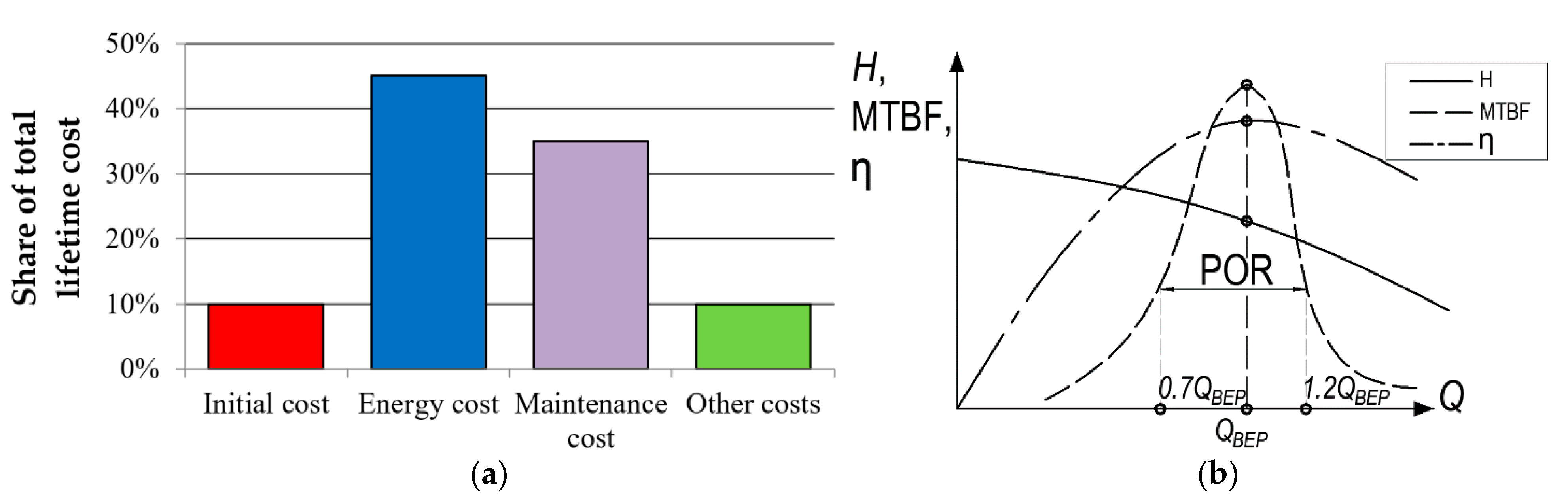
Pumps consume about 20% of the electricity generated worldwide. The largest part of the pump’s life cycle costs is the price of the electricity it consumes. Therefore, pumps are one of the most promising areas for applying energy-saving technologies. At the same time, maintenance and repair account for a significant part of the life cycle costs of a pump unit (Figure 1a). Therefore, when optimizing the overall life cycle costs, in addition to taking into account the initial cost of equipment and energy costs, it is also necessary to consider the costs of maintenance and repair, which are affected by the reliability of the pump [1]. In [2,3], it was shown that the Mean Time Between Failure (MTBF) can be used to quantify reliability. In turn, MTBF depends on the deviation between the current pump flowrate Q and the Best Efficiency Point (BEP). By analyzing the statistics of pump failures together with the deviation between the operating point and the BEP, it is possible to determine the preferred operating region (POR), within which the MTBF is sufficiently high [4,5]. According to [4], the POR is between the of 0.7∙Q_BEP and 1.2∙Q_BEP points on the Q-H characteristic (Figure 1b).

Parallel pumps are widely used in many applications, for example when high flow, high head, or wide range of flow adjustment is required. When using parallel pumps, it is possible to significantly reduce all components of the life cycle cost of a pumping station, in comparison with a single-pump unit of the same rated power [2,6]. At the same time, due to a large number of variable parameters and nonlinearity of such systems, the problems of optimizing their energy consumption, taking into account the reliability and cost of the life cycle, are complex and are still not often considered in the literature.

A wide variety of articles concern the energy efficiency issues of multi-pump systems. A number of works only consider increasing the energy efficiency of the parallel pump system, without taking into account its reliability.

In [7], for example, the optimization of multi-pump system operation is considered in order to increase the reliability and improve the efficiency of the system. For pumps operating in parallel mode, the possibility of the optimal control strategy is studied with the help of a genetic algorithm. The obtained results show that the highest efficiency is achieved by ensuring the same flowrate of two pumps. This article also studies the comparison of a system consisting of two pumps with one frequency converter, and the same system with two separate frequency converters for each pumping unit. The efficiency of the two systems is compared depending on the fluid flowrate. It is shown that the latter system has better efficiency.

In [8], an energy efficient strategy for controlling six parallel pumps is considered, each of which has a variable speed drive (VSD). It is shown that the asynchronous distributed optimal control algorithm is more efficient than synchronous methods.

Several works analyze pumping systems in terms of their energy consumption and deviation of operating points from the BEP. In [5], optimization of a single-pump unit is considered to increase its reliability using a genetic algorithm. However, a number of aspects were not considered in [5]: the optimization criterion is only the maximum service life of the pump unit; the possibility of obtaining a trade-off between reliability and energy consumption is not considered. The paper also does not consider the possibility of obtaining a better operating point by means of bypass control. The static head in the hydraulic system is assumed to be zero, which also reduces the range of cases to which the results of the work are applicable.

In [9], the efficiency and reliability of one-pump unit and two parallel pumps powered directly from the mains are compared. It is shown that in the latter case both the cost of electricity and the cost of maintenance will be significantly lower.

In [10], an analysis of a single-pump unit with a rated power of 11 kW was carried out in terms of reducing energy consumption and increasing reliability. A trade-off control method has been proposed that provides good reliability with power consumption close to the minimum. The power consumption is calculated for three cases: traditional variable speed control, control with maximum reliability, and trade-off control. It was shown that, when using the trade-off control, it is possible to significantly reduce the energy consumption of the pump unit, in comparison with the case of maximum reliability, maintaining all pump operating points within POR.

In [2], another trade-off control method was proposed using particle swarm optimization for a system of two identical parallel pumps, each of which is equipped with a frequency converter (FC). The number of the pumps in operation and the rotational speed of the pumps were selected as the optimization parameters. Energy consumption was used as the optimization criterion. The deviation between the current operating point and the BEP was used as a constrain. It was assumed that the speeds of both pumps are equal at each operating point, and a single throttle is used to adjust the hydraulic head in the common section of the pipeline of the parallel pumps. However, the results of this study are only applicable when the speed of both parallel pumps is controlled by FC. Meanwhile, in practice, the pumps operating in parallel may have no speed control, and are powered directly from the grid.

In this paper, a system with two identical parallel pumps with the rated power of 5.5 kW is considered to reduce the energy consumption of the system with the assumed limitation of the deviation of operating points from the BEP. In contrast to [2], this work considers the case when only one of the two pumps is equipped with an FC, and the other is powered directly from the grid. The considered pumping system with two motors and one frequency converter is a special case of multi-motor pumping stations with one frequency converter (multi-pump single-drive systems) for fluid machinery. Such systems are widely used in low-power electric drives [11,12]. This makes it possible to significantly reduce the initial costs of multi-unit pumping stations, while providing smooth control of their head or flow [6].

The multi-pump single-drive systems are widely used in parallel pumping stations equipped with low-power electric motors [12]. However, analysis of such systems is not very common in the literature. In such pumping systems, one frequency converter controls two or more pumps. At the same time, in contrast to systems without a frequency converter, a smooth start-up of each pump unit and a smooth flow/pressure adjustment are ensured. In contrast to the case where each pump unit is equipped with an individual frequency converter, the capital cost of the system is significantly reduced. This advantage is especially important if the system uses low-power pump units, for which the cost of the frequency converter is the largest part of the total cost, as well as in systems containing a large number of pumping units.

Such systems have only one variable speed pump. To adjust both pumps operating in parallel, bypass and throttling are applied individually. Therefore, the operating points of the pumps differ significantly from the cases when all pumps are powered by a frequency converter, as discussed in [2], or when all pumps are supplied from the mains, as discussed in [9]. Therefore, the conclusions carried out in [2] cannot be directly applied to the multi-pump single-drive systems.

Due to the wide variation in flow and head in real pumping systems, the pump operating point is very rarely located near the BEP. However, to ensure an acceptable service life, the operating point of the pump must be located in the preferred operating region (POR). According to [4], the POR is between 0.7∙Q_BEP and 1.2∙Q_BEP. This condition can be considered as a constraint when adjusting the pumping system. Therefore, this paper compares the energy consumption of the pumping system in three cases.

The first is control with minimum energy consumption, without applying any reliability constraints. In this case, the flow is adjusted by changing only the rotational speed of the first pump with FC and throttling the second pump without the speed control. When the flowrate changes from 0 to 60%, only the variable speed pump operates. To provide greater flow rates, the second pump without speed control also turns on. When two pumps run at the same time, an equal distribution of the flow between them is realized. In this case, energy consumption is minimized, but not all operating points of the pumps will be located in the POR [5].

The second is control with maximum reliability. In this case, the adjustment is performed not only by changing the speed, but also by throttling and bypassing both pumps. Using this control method, all operating points of the pumps will be located on the curve maximum service life. Due to the use of throttling and bypass, the energy consumption of the pumping system increases in comparison with the first case. When the flow rate changes from 0 to 50%, only the variable speed pump runs, then the pump without FC also turns on.

The final case is trade-off control considering the reliability constraint. The flowrate is adjusted by changing the rotational speed of the first pump, as well as throttling and bypassing both pumps. Using this control method, all operating points of the pumps will be in the range from 0.7∙Q_BEP to 1.2∙Q_BEP during the whole considered operating cycle. The chosen restriction of the flow range is based on [3]. In [3], it is shown that if the pump operating points are within this range, then the pump is moderately affected by negative factors that reduce reliability, and its resource does not decrease very much, in comparison with the best possible case when the pump is always running near the BEP (Figure 1b). When the flowrate changes from 0 to 50%, only the variable speed pump runs, then the pump without FC is also turned on.

2. Proposed Control Method for the Considered Parallel Pump System

The pump system considered is used to provide the required flowrate Q_req in an open-type hydraulic system with constant static head H_st, from point A to point B (Figure 2a) [13]. Pump P1 and motor M1 make up the first pump unit. Pump P2 and motor M2 make up the second pump unit. Only the first pump unit is equipped with the frequency converter (FC). The head that each of the pumps produces in the common pipeline can be regulated by throttles D1 and D2, respectively. Additionally, each of the pumps has an adjustable bypass track B1 and B2, respectively. By increasing the flow rates Q_b1 and Q_b2 through the bypass tracks, it is possible to regulate the flows Q_r1 = Q_p1 − Q_b1 and Q_r2 = Q_p2 − Q_b2 which flow from each of the pumps to the common pipeline, where Q_p1 and Q_p2 are the flow rates through the pumps P1 and P2, respectively.

Depending on the geometric dimensions of the pipelines (length, cross-section, shape, etc.), the physical properties of the pumped liquid (density, viscosity, etc.), and the difference in heights of the reservoirs A and B, the curve of the hydraulic system is constructed, which is described by the Equation (1) [13]:

H_SYS = H_ST + k·Q_REQ²,

(1)

where H_SYS is the required hydraulic head; H_ST is the static head; and k is the hydraulic friction coefficient of the hydraulic system.

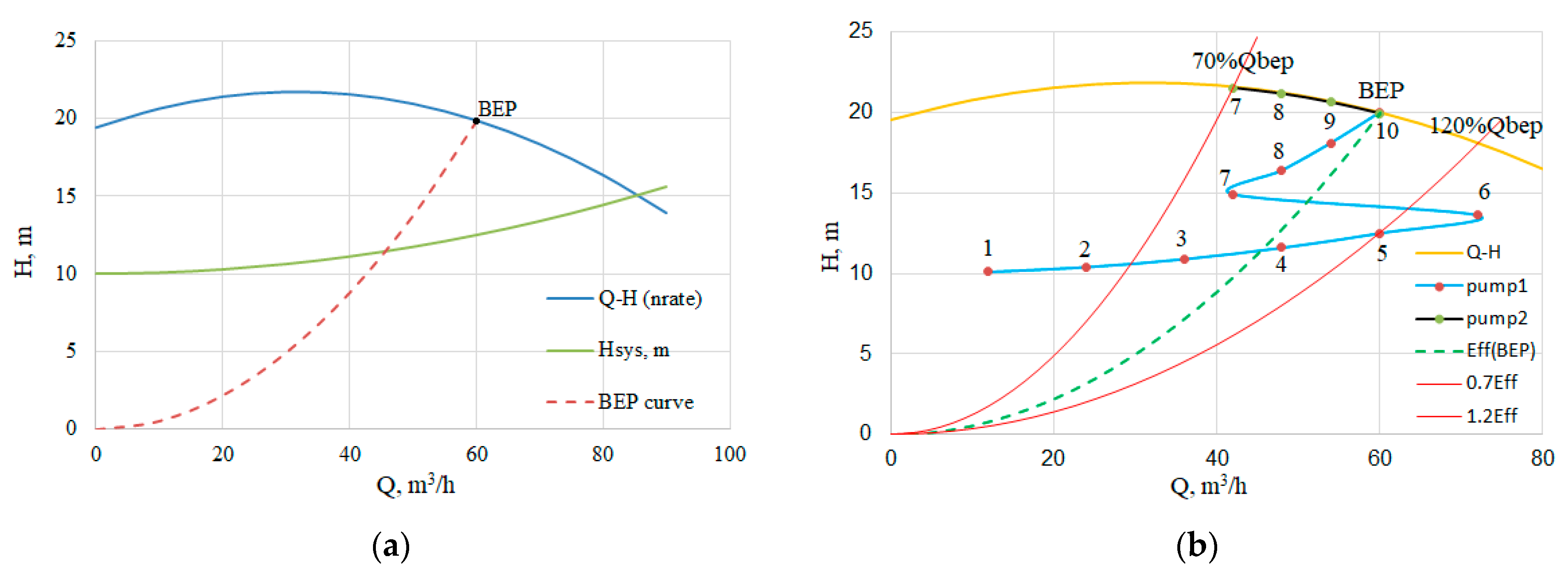
Figure 2b shows various characteristics of the system. Numbers 1 and 2 indicate the curves of the hydraulic system with a non-zero value of the static head H_ST and different values of k. Numbers 3 and 4 indicate the curves of the hydraulic system with different values of k and H_ST = 0. Number 5 marks the dashed curve on which the BEP points lie at different pump rotation speeds (BEP curve), which can be calculated using the similarity laws [2]. The selection of pumps is carried out based on the maximum values of the required flow rate and hydraulic head. In the ideal case, when the system curve matches the BEP curve (curve 5 in Figure 2b), both maximum reliability and efficiency is reached. However, in real conditions, the operating point may be located far from the BEP curve. Therefore, depending on the resulting curve of the hydraulic system, it is necessary to adjust the pump operating point to improve the reliability of the pump.

If the curve of the hydraulic system is to the right of the BEP curve (as curve 4 in Figure 2b), then adjusting the rotational speed and throttling must be used to decrease the deviation of the operating point from the BEP curve Ɵ [5]. If the curve of the hydraulic system is to the left of the BEP curve (as curve 3 in Figure 2b), then bypass control along with speed adjustment must be applied. However, the use of throttling and bypass along with adjusting the rotational speed leads to additional energy consumption. In this paper, a hydraulic system is considered, the curve of which has a position similar to curve 2 in Figure 2b. With such an alignment of the system curve and the BEP curve, both bypass and throttling along with speed adjustment are required to achieve the maximum reliability.

3. Deviation of the Flow Rate from BEP Applying the Different Control Methods

For assessing the considered control methods, in this study catalogue characteristics of the centrifugal pump Calpeda B 65/12C with the rated power of 5.5 kW and with the rated speed of 2900 rpm are considered.

Table 1. Pump H-Q characteristic.

Q, m3/h	37.8	42	48	54	60	66	75	84
H, m	22	21.5	21	20.5	20	19.5	18	15.5

shows the points of the H-Q curve of this pump [14].

The maximum required flowrate of the pump system is Q₁₀₀ = 120 m³/h. To simplify the calculations, the Q-H characteristics and characteristics of the pump mechanical power P = f (Q, s) are written in the form of two variable polynomials of the 2nd and 3rd orders, respectively [12]:

H = a·Q² + b·Q·s + c·s²;

(2)

P = c₀·Q³ + c₁·Q²·s + c₂·Q·s² + c₃·s³,

(3)

where s = n/n_rate is the rotational speed in in relative units, a = −0.0023, b = 0.1457, c = 19.45, and c₀ = −0.00032; c₁ = 0.2975, c₂ = 25.12, and c₃ = 2668 are the coefficients of polynomials (2) and (3), respectively.

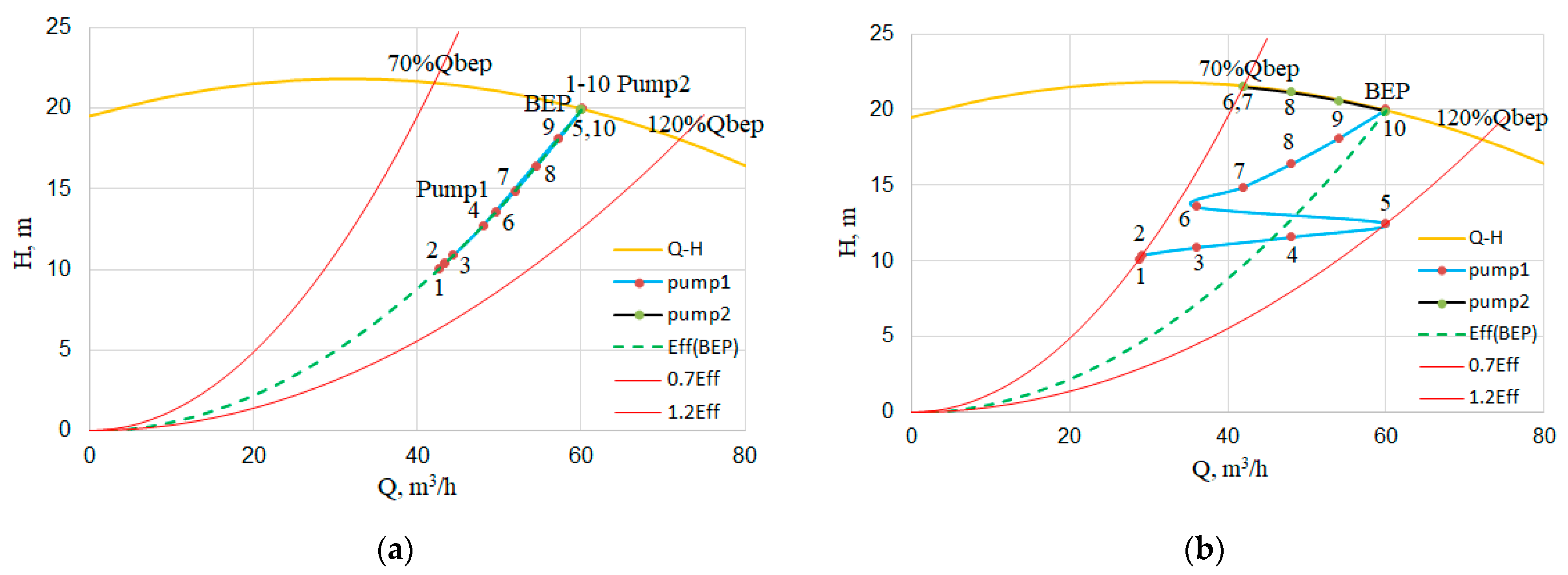
Figure 3a shows the Q-H curve of the single pump at the rated rotational speed (n_rate), hydraulic system curve and BEP curve. The BEP curve is given by the following equation:

H = k_BEP · Q²,

(4)

where k_BEP = H_BEP/Q_BEP; and Q_BEP and H_BEP are the flow and head, respectively, in BEP at n = n_rate.

First, let us calculate the characteristics of the pumping system with the minimum energy consumption control [6]. The rotational speed of the first pump is adjusted by FC. The speed of the second pump running in parallel is not controlled. With this control, the operating points of the variable speed pump are located along the curve of the hydraulic system, and the operating points of the fixed speed pump are located along the catalogue Q-H curve (Figure 3b).

Table 2. Pump system performances applying the minimum energy consumption control.

Q, %	Q, m3/h	Q1, m3/h	Q2, m3/h	H1, m	n1, rpm	H2, m	Pp1, W	Pp2, W	P1+2, kW	Eff1, %	Eff2, %	Ɵ1, %	Ɵ2, %	n2, rpm
10	12	12	-	10.1	1997	-	1039	0	1.04	31.8	-	−71.0	-	-
20	24	24	-	10.4	2006	-	1246	0	1.25	54.6	-	−42.2	-	-
30	36	36	-	10.9	2090	-	1597	0	1.60	67.0	-	−16.7	-	-
40	48	48	-	11.6	2231	-	2104	0	2.10	72.1	-	4.0	-	-
50	60	60	-	12.5	2416	-	2790	0	2.79	73.3	-	20.0	-	-
60	72	72	-	13.6	2631	-	3686	0	3.69	72.4	-	32.3	-	-
70	84	42	42	14.9	2443	21.5	2549	4011	6.56	66.9	61.4	−16.9	−30	2900
80	96	48	48	16.4	2586	21.1	3108	4205	7.31	69.0	65.8	−10.3	−20	2900
90	108	54	54	18.1	2741	20.6	3780	4388	8.17	70.5	69.1	−4.8	−10	2900
100	120	60	60	20	2905	19.9	4578	4555	9.13	71.4	71.5	−0.2	0	2900

shows the calculated characteristics of the pump system in this case. The head of the variable speed pump H = H_SYS is determined by Formula (1), the head of the fixed speed pump is determined by Expression (2), the rotational speed n is determined by Formula (5) [6], the mechanical power of the pump P is determined by polynomial (3), pump efficiency is determined by Formula (6), and the deviation of the operating points from the BEP curve is determined by Formula (7):

$$n_1=n_{rate}\cdot \frac{-b\cdot Q_1+\sqrt{{(b\cdot Q_1)}^2-4\cdot c(a\cdot Q_1{}^2-H_{sys})}}{2c},$$

(5)

η = g·ρ·Q_PUMP·H_PUMP/P,

(6)

Ɵ = (Q − Q_BEP)/Q_BEP,

(7)

where g = 9.81 m/s² is the gravitational acceleration; ρ = 1000 kg/m³ is the water density; Q_PUMP and H_PUMP are the flow and the head of the pump; and Q_BEP = f(n) is the flowrate of the pump in BEP.

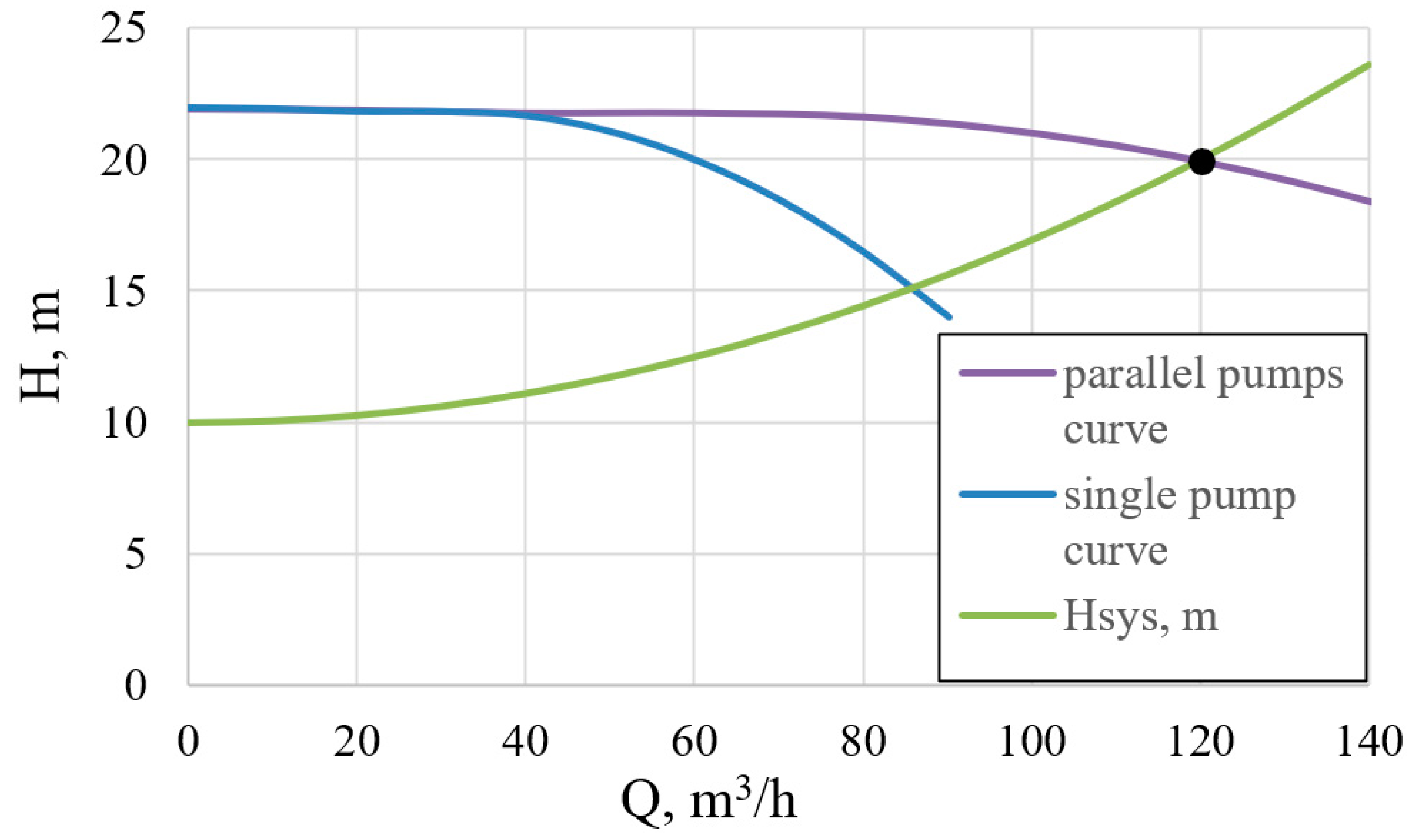
Figure 4 shows an example of finding the operating point of the considered system of two parallel pumps for the case of the highest flow rate Q = 100% = 120 m³/h. In this case, both pumps operate at a rotational speed close to the rated speed (2900 rpm, see Table 2), and their Q-H curves practically coincide (see “single pump curve”). The resulting Q-H curve (“parallel pumps curve”) is obtained by adding flow rates of the individual pumps at the same head. The operating point of the system, with a flow rate of 120 m³/h and a head of 20 m, is obtained as the intersection point of the resulting Q-H curve and the hydraulic load curve H_sys. The rest of the operating points of the parallel pump system are found in the same way. The algorithm for finding the operating point of the system when using parallel pumps is described in more detail in [6].

Based on the results shown in Figure 3b and Table 2, it can be observed that if the required flowrate is less than 30% of Q_max, as well as at 60% of Q_max (when only the one pump is running), the operating points go outside the POR, which leads to a deterioration in the pump reliability. The deviation Ɵ is in the range from 32 to 71%.

Pump operation in this range becomes unstable due to the flatness of the Q-H curve: a small deviation in the rotational speed leads to a large deviation in the flowrate. In addition, due to the unstable shape of the Q-H characteristic, the latter intersects with the hydraulic system curve in two points which leads to the occurrence of a surge. In this case, the pump operates alternately in different operating points, the whole system is unstable, the loading on the pump changes, and hydraulic shocks occur [15,16].

To ensure maximum pump reliability, the operating points of the variable speed pump must be on the BEP curve, i.e., along the dashed line shown in Figure 3a,b. The fixed speed pump must always operate in the BEP of the catalogue Q-H curve, regardless of the required flow. This can only be achieved by using all three of the above-mentioned methods of adjusting the flowrate. Therefore, according to Figure 3b operating points 1–3 and 6–9 are to the left of the BEP-curve. They must be moved horizontally until they coincide with the BEP curve. In practice, this can be achieved by increasing the pump flowrate Q_PUMP from Q_REQ to Q_BEP at the same head, i.e., Q_PUMP is increased with the same Q_REQ. The excess flow Q_B = Q_PUMP − Q_REQ flows back through the bypass to the suction pipe. Points 4 and 5 are located to the left of the BEP curve. To move these points up to the BEP curve, at the given flowrate Q_REQ, it is necessary to increase the head at the pump outlet using throttling (Figure 5a).

The required head H_REQ = H_SYS is determined using Formula (1); the flowrate Q_PUMP and the head H_PUMP are determined by Expression (8) when using bypass regulation together with speed control, and by Expression (9) when using only the speed control. The rest of the parameters are determined in the same way as in the previous case:

Q_PUMP = √(H_REQ/k_BEP); H_PUMP = H_REQ;

(8)

Q_PUMP = Q_REQ; H_PUMP = k_BEP · Q_REQ²,

(9)

Where Q_REQ and H_REQ are the required output flow and head, respectively; and Q_PUMP and H_PUMP are the flow and head of the pump, respectively.

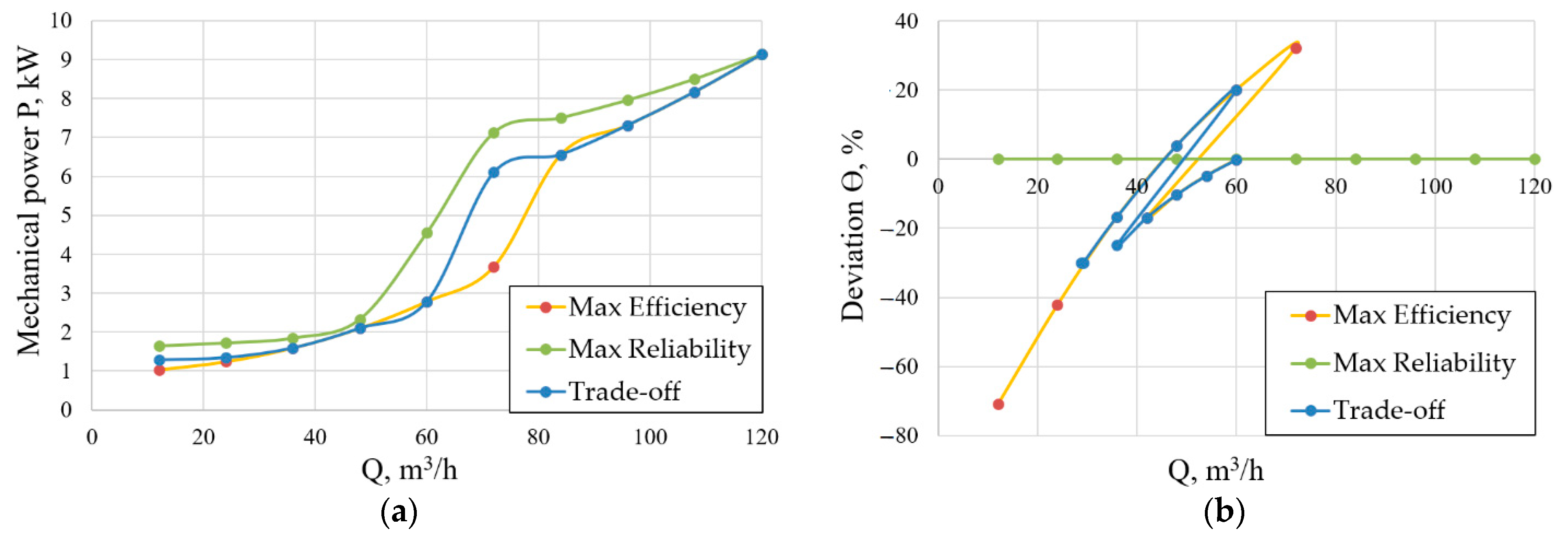
As it can be observed from the results presented in Figure 5a and

Table 3. Pump system performances applying the maximum reliability control.

Q, %	Q, m3/h	Qr1, m3/h	Hr1, m	Qp1, m3/h	Hp1, m	n1, rpm	Qr2, m3/h	Qp2, m3/h	Hp2, m	Pp1, kW	Pp2, kW	P1+2, kW	Eff1, %	Eff2, %	Ɵ1, %	Ɵ2, %	Hr2, m
10	12	12	10.1	42.7	10.1	2066	0	0	-	1.65	0	1.65	71.5	-	0	-	-
20	24	24	10.4	43.4	10.4	2096	0	0	-	1.72	0	1.72	71.5	-	0	-	-
30	36	36	10.9	44.4	10.9	2146	0	0	-	1.85	0	1.85	71.5	-	0	-	-
40	48	48	11.6	48.0	11.6	2320	0	0	-	2.33	0	2.33	71.5	-	0	-	-
50	60	60	12.5	60.0	12.5	2900	0	0	-	4.55	0	4.55	71.5	-	0	-	-
60	72	36	13.6	49.6	13.6	2397	36	60	19.9	2.57	4.55	7.13	71.5	71.5	0	0	13.6
70	84	42	14.9	51.9	14.9	2509	42	60	19.9	2.95	4.55	7.50	71.5	71.5	0	0	14.9
80	96	48	16.4	54.5	16.4	2632	48	60	19.9	3.41	4.55	7.96	71.5	71.5	0	0	16.4
90	108	54	18.1	57.2	18.1	2765	54	60	19.9	3.95	4.55	8.50	71.5	71.5	0	0	18.1
100	120	60	20.0	60.1	20.0	2907	60	60	19.9	4.59	4.55	9.14	71.5	71.5	0	0	20

, when throttling and bypass are used together with speed control, the maximum pump reliability can be achieved. The efficiency of both pumps throughout the entire range of flow regulation remains maximum (71.5%) and the operating point deviation Ɵ is zero. However, the energy consumption increases, compared to the case of the minimum energy consumption control, due to an increase in Q_PUMP when using a bypass and an increase in H_PUMP when throttling.

It is also possible to apply a trade-off control method, during which energy consumption will be reduced and, at the same time, sufficiently high reliability of the pumps will be achieved. To accomplish this, it is necessary to ensure that all pump operating points are located within the POR. According to Figure 3b, when using only the speed control, points 1, 2, and 6 are outside the POR zone. In this case, as in the case of achieving maximum reliability, points 1, 2 are moved horizontally to the right, but only to the border of the POR by bypassing (Figure 5a). Point 6 is moved within the POR using throttling. Thus, all operating points are in the POR zone. This ensures high reliability and lower power consumption. Throttling is not applied for these points.

Table 4. Pump system performances applying the trade-off control.

Q, %	Q, m3/h	Qr1, m3/h	Hr1, m	Qp1, m3/h	Hp1, m	n1, rpm	Qr2, m3/h	Qp2, m3/h	Hp2, m	Pp1, kW	Pp2, kW	P1+2, kW	Eff1, %	Eff2, %	Ɵ1, %	Ɵ2, %	Hr2, m3/h
10	12	12	10.1	28.8	10.1	1987	0	0	-	1.29	0	1.29	61.4	-	−30	-	-
20	24	24	10.4	29.2	10.4	2017	0	0	-	1.35	0	1.35	61.4	-	−30	-	-
30	36	36	10.9	36	10.9	2090	0	0	-	1.60	0	1.60	67.0	-	−17	-	-
40	48	48	11.6	48	11.6	2232	0	0	-	2.10	0	2.10	72.1	-	3.9	-	-
50	60	60	12.5	60	12.5	2416	0	0	-	2.79	0	2.79	73.3	-	20	-	-
60	72	36	13.6	36	13.6	2315	36	42	21.5	2.09	4.01	6.10	63.8	61.4	−25	−30	13.6
70	84	42	14.9	42	14.9	2443	42	42	21.5	2.55	4.01	6.56	66.9	61.4	−17	−30	14.9
80	96	48	16.4	48	16.4	2586	48	48	21.1	3.11	4.21	7.31	69.0	65.8	−10	−20	16.4
90	108	54	18.1	54	18.1	2741	54	54	20.6	3.78	4.39	8.17	70.5	69.1	−4.8	−10	18.1
100	120	60	20	60	20	2906	60	60	19.9	4.58	4.56	9.13	71.4	71.5	−0.2	0	20

shows the characteristics of the pump system applying the trade-off control. The required head of the variable speed pump H_REQ = H_SYS is determined using formula (1), the flow through the pump Q_PUMP and the head H_PUMP are determined by Expressions (10) with bypass regulation. The rest of the parameters are determined in the same way as in the previous case:

Q_PUMP =√(H_REQ/k_0.7BEP), H_PUMP = H_REQ,

(10)

where k_0.7BEP = H(0.7∙Q_BEP)/(0.7∙Q_BEP).

As Table 4 shows, when using the trade-off control, the efficiency of the pumps in the entire range of flow regulation is not less than 61.4%. The deviation Ɵ is no more than 30%, and the energy consumption is reduced compared to the case of the maximum reliability control. Figure 6a provides the comparison of mechanical power and the deviation Ɵ when using the three considered control methods.

4. Pump System Energy Consumption in the Considered Operating Cycle Applying the Different Control Methods

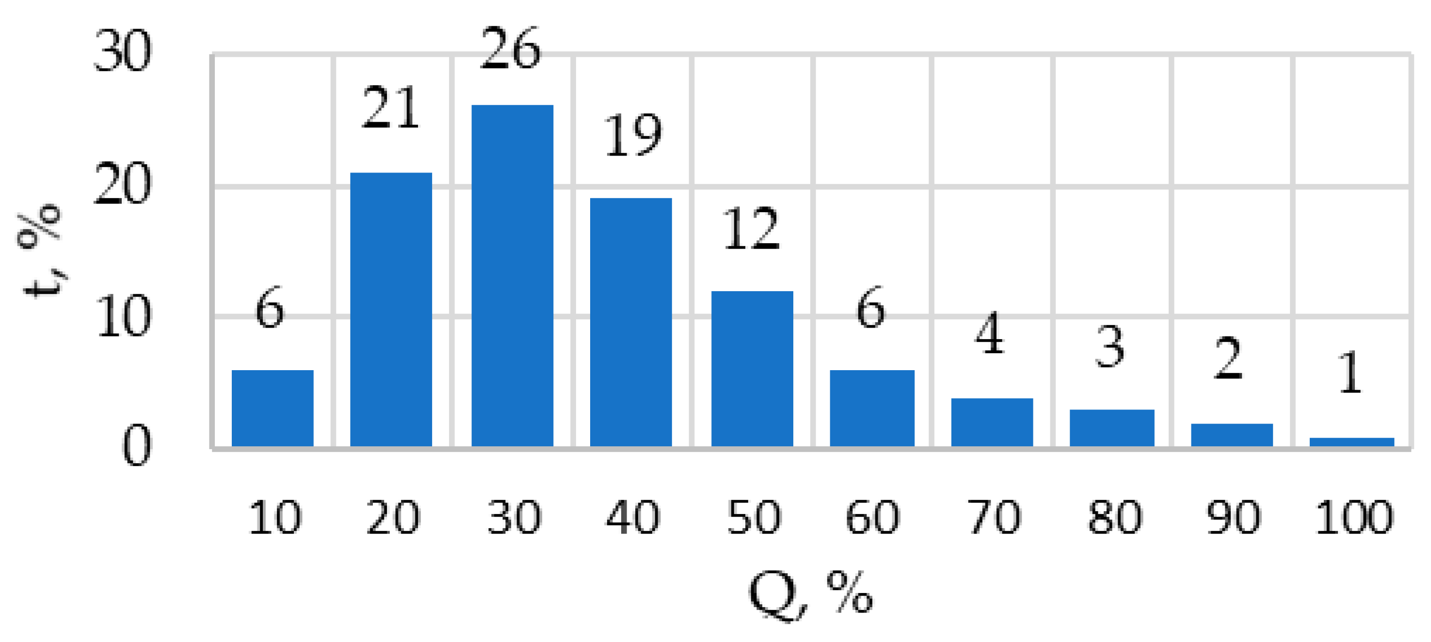
This section provides the comparison of the electric energy consumption of the pumping system using the considered control methods (Table 2, Table 3 and Table 4) when operating with a flow-time dependence typical for open-loop pumping systems [13]. This dependence is shown in Figure 7. The period of the operating cycle is taken equal to be 24 h.

It was assumed that a Sinamics G120C frequency converter, with the rated power of 5.5 kW [17], and Simotics 1LE1001-1CA6 induction motors, with the power of 5.5 kW and rated speed of 2955 rpm [18], are used in the drive of the pump system. Data from SinaSave software [19] in eight standard loading points (

Table 5. Loss data for the 5.5 kW electric drive.

Operating Point	1	2	3	4	5	6	7	8
n, %	100	100	50	50	50	0	0	0
T, %	100	50	100	50	25	100	50	25
ΔP, kW	0.9	0.42	0.63	0.27	0.18	0.5	0.21	0.13

) are used to determine the power losses and efficiency of the drive (motor plus frequency converter) in the operating points with given values of the shaft torque on T and speed n that were calculated in the previous section (Table 2, Table 3 and Table 4). The standard loading points are determined according to IEC 61800-9-2, “Adjustable Speed Electrical Power Drive Systems–Part 9-2: Ecodesign for Power Drive Systems, Motor Starters, Power Electronics and Their Driven Applications–Energy Efficiency Indicators for Power Drive Systems and Motor Starters” [20]. This data are used as the standard [20] requires manufacturers to declare the loss values for variable frequency drives at these eight operating points.

Using the data from Table 5, it is possible to find the losses in the drive at the considered operating points (Table 2, Table 3 and Table 4) using polynomial interpolation [21,22]. The results of this calculation are shown in

Table 6. Results of the loss calculation in the electric drive of the pump system applying the different control methods.

Qreq, %	Qreq, m3/h	ΔP, kW
		Minimum Energy Consumption	Maximum Reliability	Trade-Off Control
10	12	0.22	0.28	0.24
20	24	0.24	0.29	0.25
30	36	0.27	0.31	0.28
40	48	0.33	0.37	0.34
50	60	0.42	0.70	0.43
60	72	0.56	0.40	0.34
70	84	0.39	0.45	0.39
80	96	0.46	0.52	0.47
90	108	0.56	0.60	0.58
100	120	0.69	0.71	0.71

.

According to the proposed trade-off regulation principle, it is necessary to correct only the operating points which deviations Ɵ are outside the POR boundaries (Ɵ < −30% and Ɵ > 20%). As Figure 3b and Table 2 show, most of the operating points of the three pumps are already within the POR when the “maximum efficiency” regulation is applied. Therefore, when the trade-off regulation is applied, most of the operating points remain unchanged in comparison with the maximum efficiency regulation method. Therefore, the correction of these points when using the trade-off regulation does not require significant additional energy consumption at most operating points. Only for the correction of operating points 1, 2, and 6 is additional power consumption required, which is reflected in

Table 7. Results of the electric power calculation in the pump system applying the different control methods.

Qreq, %	Qreq, m3/h	Pelec, kW
		Minimum Energy Consumption	Maximum Reliability	Trade-Off Control
10	12	1.26	1.93	1.53
20	24	1.48	2.01	1.6
30	36	1.87	2.15	1.87
40	48	2.44	2.70	2.44
50	60	3.21	5.26	3.22
60	72	4.24	8.06	6.92
70	84	7.43	8.49	7.44
80	96	8.28	9.02	8.28
90	108	9.25	9.65	9.26
100	120	10.37	10.39	10.38

. This results in similar P and θ plots for the maximum efficiency and trade-off regulation methods are shown in Figure 6.

Using the results obtained (Table 2, Table 3, Table 4, Table 5 and Table 6), it is possible to calculate the electrical power consumed from the grid (P₁), the daily consumed electrical energy (E_DAY), the annual consumed electrical energy (E_YEAR), the annual energy costs (C_YEAR), and the cost of energy over the entire life cycle of the pumping unit (C_LLC) [23]:

P₁ = P_PUMP + ΔP;

(11)

$$E_{DAY}=\frac{t_{\Sigma }}{1000}\cdot {\displaystyle \sum _{i=1}^{10}\left(P_1\left(i\right)\cdot \frac{t_i}{t_{\Sigma }}\right)};$$

(12)

E_YEAR = E_DAY · 365;

(13)

C_YEAR = E_YEAR · GT;

(14)

$$C_{LCC}={\displaystyle \sum _{i=1}^w\left(\frac{C_{YEAR i}}{{\left(1+\left[y-p\right]\right)}^i}\right)},$$

(15)

where P_PUMP is the mechanical power required by the pumps; ΔP is the loss in the electric drive; t_Ʃ = 24 h is the whole operating period; t_i is the operation time of a loading point; GT = 0.2036 €/kWh is the applied grid tariffs for non-household consumers for Germany in the second half of 2019 [24]; C_YEAR is the annual electricity cost; C_{YEAR i} is the annual electricity cost for i-th year; y = 0.06 is the interest rate; p = 0.04 is the expected annual inflation; and w = 20 years is the lifetime of the pump system.

The difference in the lifetime energy cost in kEUR and in % is calculated as:

ΔC_LLC = C_LLC − C_{LLC MAX EFF};

(16)

ΔC_LLC = 100% ∙ (C_LLC − C_{LLC MAX EFF})/C_{LLC MAX EFF},

(17)

where C_LCC is the lifecycle electricity cost of the considered pump system; C_{LCC MAX EFF} is the lifecycle electricity cost of the pump system with the minimum energy consumption control. Table 7 and

Table 8. Results of the life cycle costs for various considered cases.

Control Method	Minimum Energy Consumption	Maximum Reliability	Trade-Off Control
EDAY, kWh	67.47	87.19	72.39
EYEAR, kWh	24,628	31,825	26,421
CYEAR, EUR	5014	6479	5379
CLLC, kEUR	81.99	105.95	87.96
ΔCLLC, kEUR	-	23.96	5.97
ΔCLLC, %	-	29.2	7.3

show the calculation results based on Equations (11)–(17).

According to the data in Table 7, it can be observed that the energy consumption when using control with maximum reliability is significantly higher than when using control with minimum energy consumption over the entire flow range from 10 to 90%. At the same time, when using trade-off control, energy consumption is increased only at loading points of 10, 20, and 60% of the maximum flow. Moreover, even at these points, energy consumption is still lower than in the case of maximum reliability control. The comparison of the lifecycle energy consumption provided in Table 8 shows that applying the maximum reliability control leads 29.2% more power consumption than the minimum energy consumption without any reliability constraint. At the same time, when trade-off control is applied, the power consumption is only 7.3% higher.

5. Conclusions

In this paper, an analysis of the energy consumption of a pumping system consisting of two 5.5 kW pumps operating in parallel is carried out, considering the reliability constraints. One 5.5 kW variable frequency induction motor and one 5.5 kW fixed frequency induction motor are used in the drive of the pump system.

Energy consumption of the system when three methods of flowrate control are applied is compared: with minimum power consumption, with maximum reliability, and trade-off control. Comparison of energy consumption in the considered cases shows that energy consumption is 29.2% higher with maximum reliability control compared to minimum energy consumption control without any reliability constraints. At the same time, when trade-off control is applied, the power consumption is only 7.3% higher. It can be concluded that the proposed trade-off control is promising in terms of minimizing the overall lifetime costs of the parallel pumping system when both energy costs and maintenance and repair costs are considered.