Characterization of Export Regimes in Concentration–Discharge Plots via an Advanced Time-Series Model and Event-Based Sampling Strategies

Abstract

Currently, the export regime of a catchment is often characterized by the relationship between compound concentration and discharge in the catchment outlet or, more specifically, by the regression slope in log-concentrations versus log-discharge plots. However, the scattered points in these plots usually do not follow a plain linear regression representation because of different processes (e.g., hysteresis effects). This work proposes a simple stochastic time-series model for simulating compound concentrations in a river based on river discharge. Our model has an explicit transition parameter that can morph the model between chemostatic behavior and chemodynamic behavior. As opposed to the typically used linear regression approach, our model has an additional parameter to account for hysteresis by including correlation over time. We demonstrate the advantages of our model using a high-frequency data series of nitrate concentrations collected with in situ analyzers in a catchment in Germany. Furthermore, we identify event-based optimal scheduling rules for sampling strategies. Overall, our results show that (i) our model is much more robust for estimating the export regime than the usually used regression approach, and (ii) sampling strategies based on extreme events (including both high and low discharge rates) are key to reducing the prediction uncertainty of the catchment behavior. Thus, the results of this study can help characterize the export regime of a catchment and manage water pollution in rivers at lower monitoring costs. We propose a simple stochastic time-series model to represent the export regime of a catchment beyond simple regression. We propose how to get the required data with the least effort when the use of high-frequency in situ analyzers is not feasible or restricted. Sampling strategies based on extreme events are essential for reducing the prediction uncertainty of the catchment behavior.

1. Introduction

The way a catchment releases and metabolizes a compound defines the export regime (or behavior) of the catchment regarding this compound. Export regimes can be classified as chemodynamic when concentration varies with discharge (positively or negatively), and as chemostatic when the concentration is not affected by discharge [1,2,3,4,5,6,7]. Chemodynamic export regimes can be classified as dilution behavior and mobilization behavior. During rainfall, a catchment demonstrates dilution behavior if the compound concentration is diluted with high discharge. Contrarily, the catchment shows mobilization behavior if the compound concentration increases with discharge. This can occur for compounds mobilized by fast runoff components (e.g., nitrate by interflow, particle-bound pollutants by surface runoff) [7]. On the other hand, a chemostatic export regime presents a washout of pollutants at a relatively constant concentration (the compound concentration varies only slightly with discharge).

One can characterize the export regime of an entire catchment by collecting water samples in the catchment river outlet together with river discharge measurements. However, budgetary restrictions usually limit field campaigns. For this reason, it is crucial to design sampling strategies effectively. Sampling strategies can follow either high- or low-frequency approaches. Low-frequency series (samples by week or month) have commonly been used to characterize the concentration–discharge (C–Q) relationship of a catchment [4,7,8,9]. For example, Godsey et al. [4] used hydrochemical data of 59 sites, with more than 30 years of data, but with only five to seven water samples a year. Musolff et al. [7] used 16-year time series of monthly and bi-monthly samples at gauging stations to predict export behavior. In comparison to low-frequency sampling, high-frequency sampling (e.g., hourly samples) decreases the uncertainty of export estimates [10] and water quality parameters [11]. Some examples of studies that use high-frequency sampling are Bowes et al. [12], Evans and Davies [13], Floury et al. [14], Grimaldi et al. [15], Jones et al. [16], Liu et al. [17], Ockenden et al. [18], Rusjan et al. [19], and Schwientek et al. [20]. Nevertheless, both low- and high-frequency sampling approaches can provide insightful information on the catchment, e.g., [3,21].

Export regimes of a catchment are commonly described by a simple linear regression slope of log-concentrations ($lo{g}_{10}C$) versus log-discharges ($lo{g}_{10}Q$) measured in the river at the catchment outlet. The slope value of this power-law relationship defines the export regime of the catchment. A slope of negative value corresponds to dilution-type catchments, and a slope of zero corresponds to the chemostatic type [4], whereas the mobilization type shows a positive relationship between $lo{g}_{10}Q$ and $lo{g}_{10}C$ [3,4,5,6,7]. Therefore, linear regression can provide a beneficial water quality metric via the slope of $lo{g}_{10}C$-$lo{g}_{10}Q$.

However, the catchment has memory of its past due to the involved time scales of runoff formation, contaminant release, and reactive catchment-scale transport [13]. Many studies look at the effects of hysteresis on compound exports [22,23,24,25,26]. Hysteresis means that concentrations depend not only on discharge but also on showing an apparent dependency on past concentration values. Several studies capture hysteresis metrics to explain hysteresis loops produced during storms [27,28,29,30]. Thus, many catchments show temporal hysteresis that defies linear regression assumptions [31]. These hysteresis effects profoundly contradict the “residuals are independent errors” assumption that forms the basis of classical least squares regression. In simpler words, the remaining scatter of data points around the regression line should at least be uncorrelated with zero mean and a constant variance. Yet, temporal hysteresis means that the residuals are autocorrelated in time. With these assumptions violated, regression results can be suboptimal and biased, as well as foster incorrect conclusions.

To overcome the limitations of linear regression, different alternatives have been developed. For example, some methods are able to model C–Q relationships that vary with time, discharge, and season. One of these approaches is the WRTDS model [32], which is extensively used by the United States Geological Survey (USGS). The WRTDS model can analyze long-term surface-water-quality datasets by using weighted regression of concentrations on time, discharge, and season. Thus, WRTDS aims at interpolating low-frequency concentration time series (often monthly) at the scale of discharge time series (often daily), but not the characterization of export regimes. Also, the sample collection period must be at least 20 years, and a minimum of 200 samples is needed. These conditions are seldom met in most water-quality time series.

A modified and improved version of WRTDS, which gets better predictions of riverine concentration and flux, was developed by Zhang et al. [33] and Zhang & Ball [34]. Another more recent alternative methodology is the two-sided affine power scaling relationship by Tunqui et al. [35], which produced better results than the linear regression. Underwood et al. [36] applied Bayesian inference to estimate segmented regression model parameters and identify the export regime. Qian et al. [37] showed that a Bayesian approach could improve the predictions of nutrient loads.

Other recent studies have taken advantage of high-frequency time series to study the C–Q relationship. For example, Bieroza & Heathwaite [22] studied the variability of the phosphorous C–Q relationship by applying fuzzy logic models, and looked into the hysteresis of the phosphorous export.

To provide information about the processes regulating the export, many recent studies have shown that sampling strategies based on events or seasonality are deeply advantageous [5,6,22,30,34,36,38,39,40,41,42,43]. These event studies were focused on discharge time series (e.g., recession time series) such as in Jachens et al. [39], as well as combined with solute time series (e.g., C–Q studies) such as in Knapp et al. [5]. For example, Minaudo et al. [40] introduced a new model to account for different temporal scales that correspond to fast and slow events (storms and seasonal, respectively). Their results showed that apparent C–Q relationships could not only be different, but even opposite depending on the scale considered. Other recent studies used autoregressive time-series models to fit high-frequency data to decipher the dynamics of compound exports [16,18].

Nevertheless, hysteresis effects can only be detected when high-frequency observations are taken, since they are overlooked with low-frequency strategies [6,13,44]. Additionally, high-frequency measurements can be resource intensive (labor and economically) and challenging to apply at many field sites, especially during high-flood events [5].

Therefore, in this manuscript, we propose a new method to model C–Q relationships beyond simple regression. Additionally, we determine which observation strategies produce better predictions with the least effort (i.e., with fewer samples) when the use of high-frequency in situ analyzers is not available or restricted. For this purpose, we introduce a simple stochastic time-series model (regime-and-memory model, RMM) for concentrations in the river that accounts for fluctuating release and transport with memory, using an autocorrelation over time. One explicit parameter of our model represents the export regime. This parameter can morph the model among chemostatic-type and chemodynamic-type catchment behaviors, and it resembles the regression slope in plots of $lo{g}_{10}C$ versus $lo{g}_{10}Q$. To search for the best sampling strategies, we applied retrospective optimal design of experiments (ODE), as in [45]. In our specific case, retrospective means thinning out an exhaustive time series from high-frequency in situ analyzers to only a few samples.

Overall, the contributions of our work are fourfold: (i) We introduce a simple stochastic time-series model to characterize the export regime of a catchment subject to hysteresis; (ii) We demonstrate the robustness of our model even with only small data sets; (iii) We explore how many C–Q samples can be enough to characterize the export regime of a catchment sufficiently well; and (iv) We recommend sampling strategies that optimize the characterization of the export regime with the least sampling effort. For illustration purposes, we use a high-frequency data series of collected nitrate concentrations. They were collected with an in situ analyzer in the Ammer catchment in southwestern Germany. The available data [20] span a total period of nine months, with hourly observations. They include nitrate concentrations and discharge rates with over 6500 measurements in total.

Accordingly, this paper is organized as follows: In Section 2, we first explain our stochastic time-series model. Then, we explain how to infer the parameters of our model from the whole time series and how we thin out data to reduce them towards different sampling strategies. In Section 3, we introduce the observed data and catchment used for this study. In Section 4 and Section 5, we present and discuss, respectively, our results. Finally, we disclose our conclusions in Section 6.

2. Methodology

Throughout this study, we will consider $-lo{g}_{10}C$ versus $lo{g}_{10}Q$ in the following, instead of $lo{g}_{10}C$ for mathematical convenience in model building. The slope in corresponding plots is α in Equation (1), the parameter that describes the export regime in our model. For this study, we disregard a negative relation α (mobilization behavior) between $lo{g}_{10}Q$ and $-lo{g}_{10}C$, since the Ammer catchment misses this component as seen in Schwientek et al. [20] and Section 3. However, both the model and methodology can cover the full range of α (chemostatic, dilution, and mobilization behavior).

2.1. Regime and Memory Model (RMM)

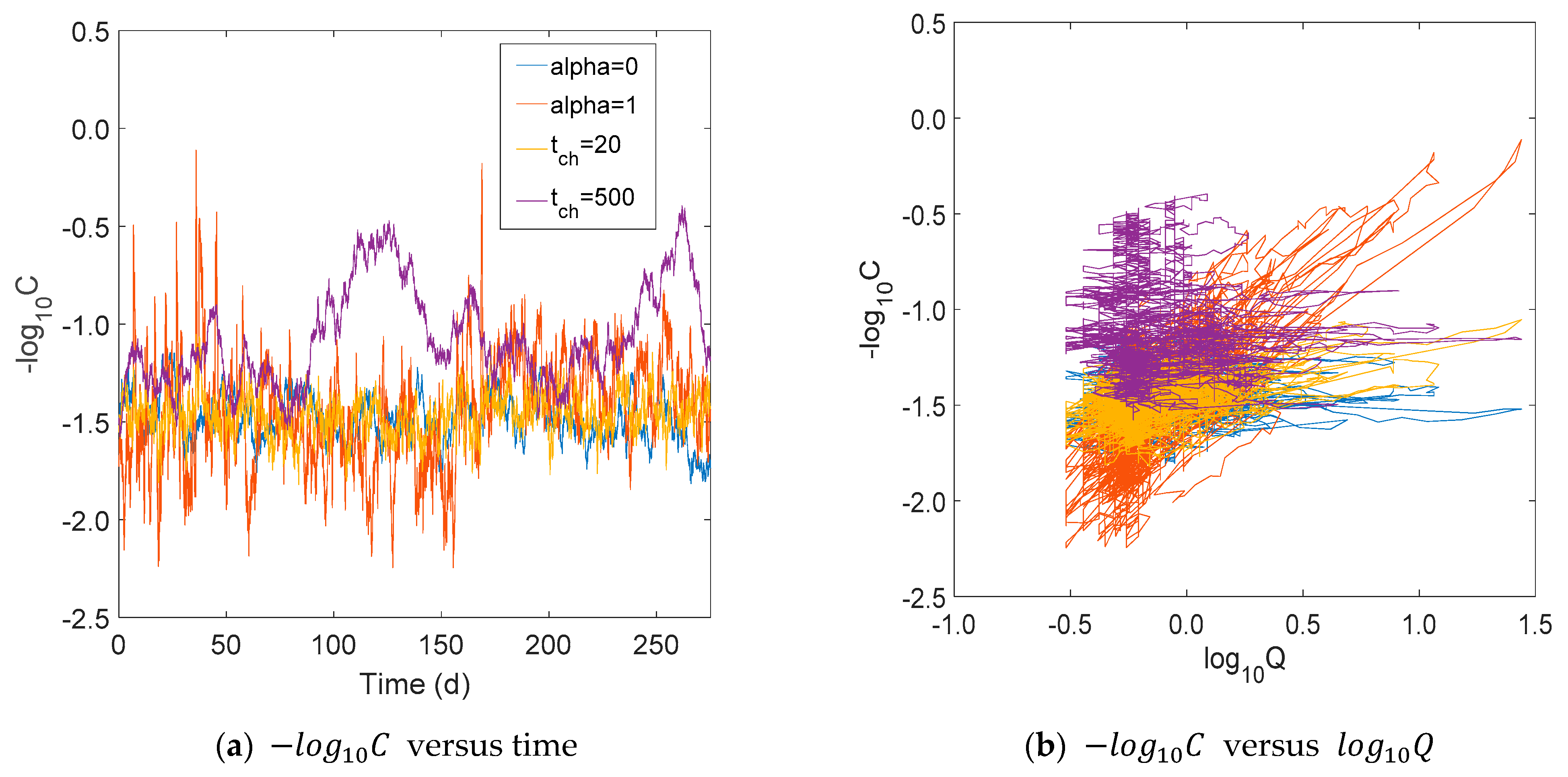
To represent the evolution of concentration versus time, we use a simple stochastic time-series model for nitrate in the river. Our model has an explicit morphing parameter α. This parameter allows a transition of the model between chemostatic-type and chemodynamic-type behavior of the headwater catchment:

$$C_t=\frac{k_t}{Q_t{}^{\alpha }}$$

(1)

In Equation (1) and throughout this manuscript, we refer to $\gamma$ (=−α) as the export regime $\in \left[-1,0\right]$ [-] ($\alpha \in \left[0,1\right]$ [-]), C is concentration ($\in {\Re }^{+}, \left[\mathrm{M}/{\mathrm{L}}^3\right]$), Q is the discharge rate ($\in {\Re }^{+}, \left[{\mathrm{L}}^3/\mathrm{T}\right]$), and $k$ is the apparent release rate $\left(\in {\Re }^{+}, ⌈\frac{M}{L^3}{\left(\frac{L^3}{T}\right)}^{\alpha }⌉\right)$. The subscript t indicates that parameters/variables depend on the current time t.

When $\alpha \approx$ 0 ($\gamma \approx$ 0), the catchment shows a chemostatic export regime, e.g., concentration only depends on the apparent release rate, which then has units of a (fixed) concentration $\left[\mathrm{M}/{\mathrm{L}}^3\right]$. When $\alpha$ is positive (γ < 0), the catchment shows a dilution behavior, presenting an anti-proportional dependence on the discharge rate. In the limit case of α = 1 ($\gamma \approx$ −1), k assumes units of a mass flow rate [M/T].

To ensure that k is never negative, we assume that k follows a lognormal distribution with mean m_k and variance $v_k$. Furthermore, we assume that k_t follows (over time) an auto-regressive model of order one (AR(1), [46]) in order to account for the dominant characteristic time scale of release and chemical turnover in the catchment. Thus, the AR(1) model is commensurate with the source strength and includes effects such as hysteresis or event-to-event variations of source availability.

Setting $\log \left(k\right)$ = $Y$, we can define an AR(1) for Y as:

$$Y_t=c+\lambda Y_{t-1}+{\epsilon }_t$$

(2)

where $\lambda$ $\in \left[0, 1\right)$ is a correlation parameter to account for the correlation between concentrations at the current time and previous times; c is a constant that is responsible for the mean; and ε is a white-noise time series, following a normal distribution with mean equal to 0 and a standard deviation of ${\sigma }_{\epsilon }$, $N\left(0,{\sigma }_{\mathsf{\epsilon }}\right)$. The AR(1) is a stochastic model with mean and variance given by:

$$m_Y=\frac{c}{1-\lambda }$$

(3)

$$v_Y=\frac{{\sigma }_{\mathsf{\epsilon }}{}^2}{1-{\lambda }^2}.$$

(4)

As seen in Mehne and Nowak [47], the characterization of an AR(1) in calibration/inferences is made more convenient and intuitive by defining a characteristic time t_ch, and the mean and variance of k, respectively, m_k and $v_k$. The characteristic time is defined as

$$t_{ch}=-1/\ln \lambda ,$$

(5)

and the relationships between $m_Y$, $v_Y$ and m_k, $v_k$ are the well-known moment relations for the lognormal distribution [48]:

$$m_Y=\ln \left(\frac{m_k{}^2}{\sqrt{v_k+m_k{}^2}}\right)$$

(6)

$$v_Y=\ln \left(\frac{v_k}{m_k{}^2}+1\right)$$

(7)

Equations (6) and (7) allow the adjustment of $log\left(AR\left(1\right)\right)$ into more understandable units of k, i.e., [M/L³] or [M/T] rather than for $Y=\log \left(k\right)$. Therefore, with only four parameters (α, m_k, v_k, and t_ch), we can represent concentrations versus time.

2.2. Bayesian Parameter Inference of Full Time-Series Data

Equations (1)–(7) define a stochastic time-series model for concentration, i.e., a model that can generate many random time series. Its relevant properties can be controlled by the choice of values for α, t_ch, m_k, v_k, and by using a given time series for Q_t. Thus, the next step is to fit the model to the observed data of concentration C_t. Due to the stochastic randomness implied for C_t by k_t (explicit by the white noise ε_t in Equation (2)), this is achieved by choosing parameter values such that the resulting model is most likely to generate good-fitting random C_t time series. This parameter choice is subject to a list of plausibility arguments for admissible parameter values.

The framework most suitable for this task is Bayesian parameter inference, as in [49]. In the heart of Bayesian inference lies Bayes’ theorem

$$p\left(\mathit{\theta }|\mathit{y}\right)=\frac{p\left(\mathit{y}|\mathit{\theta }\right) p\left(\mathit{\theta }\right)}{p\left(\mathit{y}\right)}.$$

(8)

where $\mathit{\theta }$ denotes the parameters to be inferred (α, t_ch, m_k, v_k) and y denotes the measurement data (Q, C). The prior $p\left(\mathit{\theta }\right)$ represents our belief (or knowledge) about the parameters before seeing any data and has to be chosen by us (

Table 1. Prior PDFs for uncertain parameters of the simple stochastic model.

Parameter (Unit)	Distribution	Mean	Standard Deviation	Min. Value	Max. Value
α (/)	uniform	-	-	0.0	1.0
tch (h)	lognormal LN(μ, σ) = LN (4.35, 0.65)	95.7	71.7	-	-
$m_k$$\left(\frac{mg}{l}{\left(\frac{m^3}{h}\right)}^{\alpha }\right)$	uniform	-	-	1	40
$\sqrt{v_k}$$\left(\frac{mg}{l}{\left(\frac{m^3}{h}\right)}^{\alpha }\right)$	uniform	-	-	1	6.32

). The first term on the right-hand side, $p\left(\mathit{y}|\mathit{\theta }\right)$, is the likelihood of observing the data for the given parameters. The term in the denominator, p(y), is independent of the parameters $\mathit{\theta }$, and therefore does not need to be computed. The result is the posterior distribution $p\left(\mathit{\theta }|\mathit{y}\right)$, which expresses our updated (calibrated) belief about the parameters after seeing the data y.

Following this, we choose a prior distribution for our parameters and derive an expression for the likelihood. After that, we explain how to obtain a sample from the posterior distribution via Markov Chain Monte Carlo (MCMC) sampling.

2.2.1. Prior Distributions

Bayesian parameter inference treats unknown parameter values as random variables and formulates plausibility arguments as prior probability distribution functions (PDF) (Table 1). Then, it updates these distributions to posterior distributions based on the available observation data.

We assumed that we were clueless about the export regime α and we only discarded mobilization behavior as justified in Section 3. Thus, we adopted a uniform distribution between the two extreme values of chemostatic and pure dilution behavior ($\alpha$ $\in$ [0,1]).

For the characteristic time t_ch, we assumed that concentrations in the river present roughly weekly cycles (e.g., due to weekly cycles in the release of wastewater treatment plants, which are in turn triggered by cycles in known activities) with a mean equal to four days (m_tch = 95.7 h) and a standard deviation of three days (s_tch = 71.7 h). Thus, the 95% confidence interval was about [1 d, 14 d]. Because t_ch must be positive, we chose once again a lognormal distribution. The corresponding parameters of the lognormal distribution LN(μ, σ) followed from respective copies of Equations (6) and (7), resulting in μ_tch = 4.35 and s_tch = 0.65.

We also assumed little prior information for the mean m_k, and variance v_k of the apparent release rate k, so we chose uniform distributions. We will discuss the mean m_k first. For α = 0, it corresponds to the long-term mean of nitrate concentrations. For an average discharge rate of 0.87 m³/s (Section 3), if we rounded this to ≈1 m³/s, then concentration C = k (Equation (1)) for both extreme values of α. Therefore, we can interchange C and k in the following discussion.

We assumed that the expected values of k (e.g., m_k) within the river were between pristine water (≈1 mg/L) and the effective average of the undiluted, agriculturally shaped groundwater in the Ammer catchment (≈40 mg/L, as observed as integral catchment output during baseflow by Schwientek et al. [20]). Finally, we will discuss the standard deviation $\sqrt{v_k}$ of k. For α = 0, it controls the amplitude of fluctuations in nitrate concentrations. We assumed a uniform distribution between 1 and 6.32, because we could expect both an almost constant k and a dynamic k.

2.2.2. Likelihood

To compute the likelihood, we used the following semi-analytical method. It calculates so-called depreciated increments between Y_t and Y_t−l, where l is the lag distance along time between two observations. For example, the data we used comprehended 6604 hourly samples. Between the third and the first samples, the lag time was 2. Therefore, if the whole time series is taken into account, then the lag time between two observations is l = 1. Thinning out to half the sampling rate corresponds to l = 2. Irregular sampling triggers individual lag values between consecutive data values.

We assumed that $\mathit{\theta }$ = (α, t_ch, m_k, and v_k) were currently proposed trial values. We then wanted to compute the likelihood for data from the time series y = (Q, C) for the trial values $\mathit{\theta }$. Note that y can include the whole high-frequency series of data or only a short list of observations at various lag times.

Using Equation (1), we could transform these two time series of Q and C into a time series of k_t. Then, by applying the log, we obtained a time series of Y_t. Next, we calculated $\lambda =1/t_{ch}$ (Equation (5)), and then c and ${\sigma }_{\epsilon }$ from m_Y and v_Y. We did so by first solving Equations (6) and (7), and then Equations (3) and (4). Before computing the depreciated increment between two observations, we wanted to get a Y₀ zero-mean AR(1); therefore, we removed the mean m_Y (Equation (3)) from Y:

$${\mathit{Y}}_0=\mathit{Y}-m_Y$$

(9)

Then, the depreciated increments X_l can be computed:

$${\mathit{X}}_l={\mathit{Y}}_{\mathit{t}}-{\lambda }^l{\mathit{Y}}_{t-l}={\displaystyle \sum }_1^l{\lambda }^{\left(l-1\right)}{\epsilon }_{t-l}$$

(10)

Equation (10) shows that the X_l are mutually independent, as they are sums of non-overlapping segments from the white-noise series ε_t. The variance and corresponding standard deviation of the depreciated increment are, respectively:

$${\mathit{v}}_{X_l}={\displaystyle \sum }_1^l{\lambda }^{\left(l-1\right)}{\sigma }_{\epsilon }^2$$

(11)

$${\mathit{\sigma }}_{X_l}=\sqrt{{\mathit{v}}_{X_l}}$$

(12)

After the rearrangements, the likelihood $p(\mathit{y}|\mathit{\theta })$ is now the probability density value of X_l, which in turn is given by the multivariate normal distribution:

$$\mathrm{p}\left(\mathit{y}|\theta \right)={{\displaystyle \prod }}_{t=0}^{t=n_t-1}\mathrm{p}\left({\mathit{X}}_{\mathit{l}}|\mathit{\theta }\right)·p\left({\mathit{X}}_{\mathit{l}}\right)·d{\mathit{X}}_{\mathit{l}},$$

(13)

where n_t is the total number of samples of the considered series (here n_t = 6604 when using l = 1). In Equation (13), we can use the simple product rule due to independence within the time series of X_l. Finally, the likelihood term $\mathrm{p}\left({\mathit{X}}_{\mathit{l}}|\mathit{\theta }\right)$ in Equation (13) is given by

$$\mathrm{p}\left({\mathit{X}}_{\mathit{l}}|\mathit{\theta }\right)=\frac{1}{\sqrt{2\mathsf{\pi }{\mathit{\sigma }}_{X_l}^2}}·\exp \left(\frac{{\left({\mathit{X}}_{\mathit{l}}-0\right)}^2}{2{\mathit{\sigma }}_{X_l}^2}\right),$$

(14)

which is the normal distribution for X_l implied by the chosen priors and the above equations.

2.2.3. Sampling from the Posterior

With the prior and likelihood in place, we could then sample from the posterior distribution via MCMC sampling. Here, we explicitly coded MCMC in Matlab [50]. The scaling factor for the MCMC proposal was constructed as an adjustable fraction of the posterior standard deviation to get an acceptance rate of approximately 27% (the optimal acceptance ratio for four dimensions according to Gelman et al. [51]). Since the posterior standard deviation is only known after the MCMC is run at least once, we used a burn-in run of the MCMC to obtain good scaling factors for the productive final part of the MCMC.

The posterior marginal PDF of α, $\mathrm{p}\left(\alpha |{\mathit{y}}_d\right),$ is again given by Bayes’ Theorem [49]:

$$\mathrm{p}\left(\alpha |{\mathit{y}}_d\right)\propto \int \mathrm{p}\left({\mathit{y}}_d|\alpha ,{\mathit{\theta }}_{-\alpha },X_l\right)p\left(\alpha ,{\mathit{\theta }}_{-\alpha },X_l\right)\mathrm{d}{\mathit{\theta }}_{-\mathit{\alpha }}\mathrm{d}{X}_l={\mathrm{p}}^{*}\left(\alpha |{\mathit{y}}_d\right).$$

(15)

where $p\left({\mathit{y}}_d|\alpha ,{\mathit{\theta }}_{-\alpha },X_l\right)$ is the likelihood of the observed data given α, the remaining parameters ${\mathit{\theta }}_{-\alpha }$ and X_l, and $p\left(\alpha ,{\mathit{\theta }}_{-\alpha },X_l\right)$ is the prior of the parameters and X_l. For simpler discussion, we reduced the sample to a point-estimate by computing the posterior mean from the posterior samples:

$$\mathit{\theta }=E[\mathit{\theta }|\mathit{y}] \approx \frac{1}{N}{\displaystyle \sum }_{i=1}^N{(\theta |y)}_i$$

(16)

where N is the length of the MCMC. We used N = 10,000 and N = 100,000 for the burn-in and the productive part of the MCMC, respectively. Finally, we could compute an inferred truth value α_full from the full data set, and values ${\alpha }_{post,d}$ for various sampling designs d.

2.3. Retrospective Optimal Design of Experiments (ODE)

The objective of our optimal design was to minimize the error $\varnothing$ in estimating the parameter α:

$$d_{opt}=\arg \underset{\mathrm{d}\in D}{\mathit{min}}{\varnothing }_{\alpha }\left(d\right)$$

(17)

where D is a set of considered design strategies, d is any considered design, d_opt is the best design among D, and ${\varnothing }_{\alpha }\left(d\right)$ is the squared error in estimating α for design d (as ${\alpha }_{post,d}$) when compared to α_full:

$${\varnothing }_{\alpha }\left(d\right)={\left({\alpha }_{full}-{\alpha }_{post,d}\right)}^2$$

(18)

In summary, when we thinned out the time-series data, only including data as specified by design d, we inferred α and hoped that this ${\alpha }_{post,d}$ would remain close to α_full (α inferred with full time-series data). We also assessed whether ${\alpha }_{post,d}$ had little remaining uncertainty as expressed by intervals in its distribution $\mathrm{p}\left(\alpha |{\mathit{y}}_d\right)$ according to Equation (15).

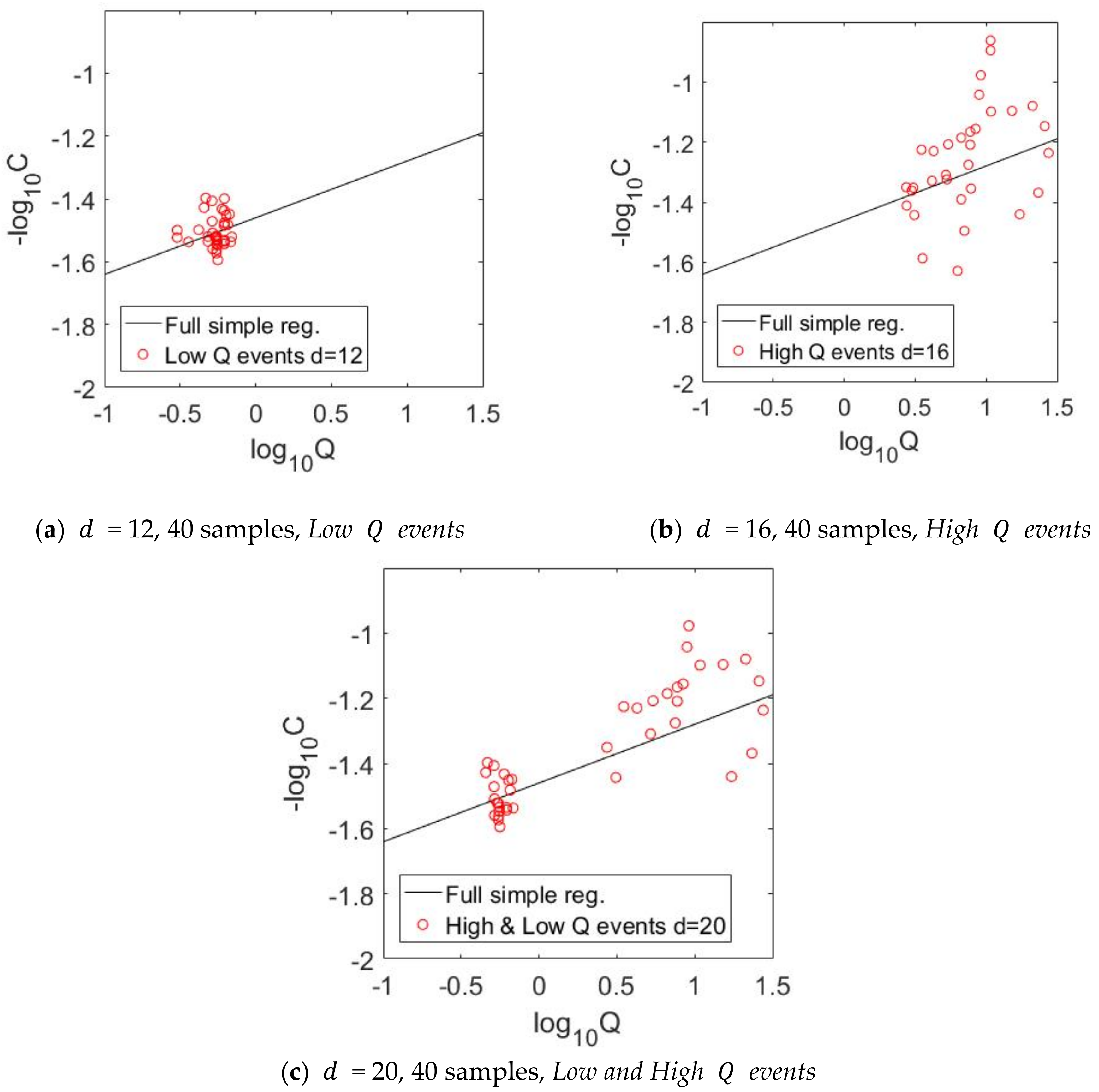
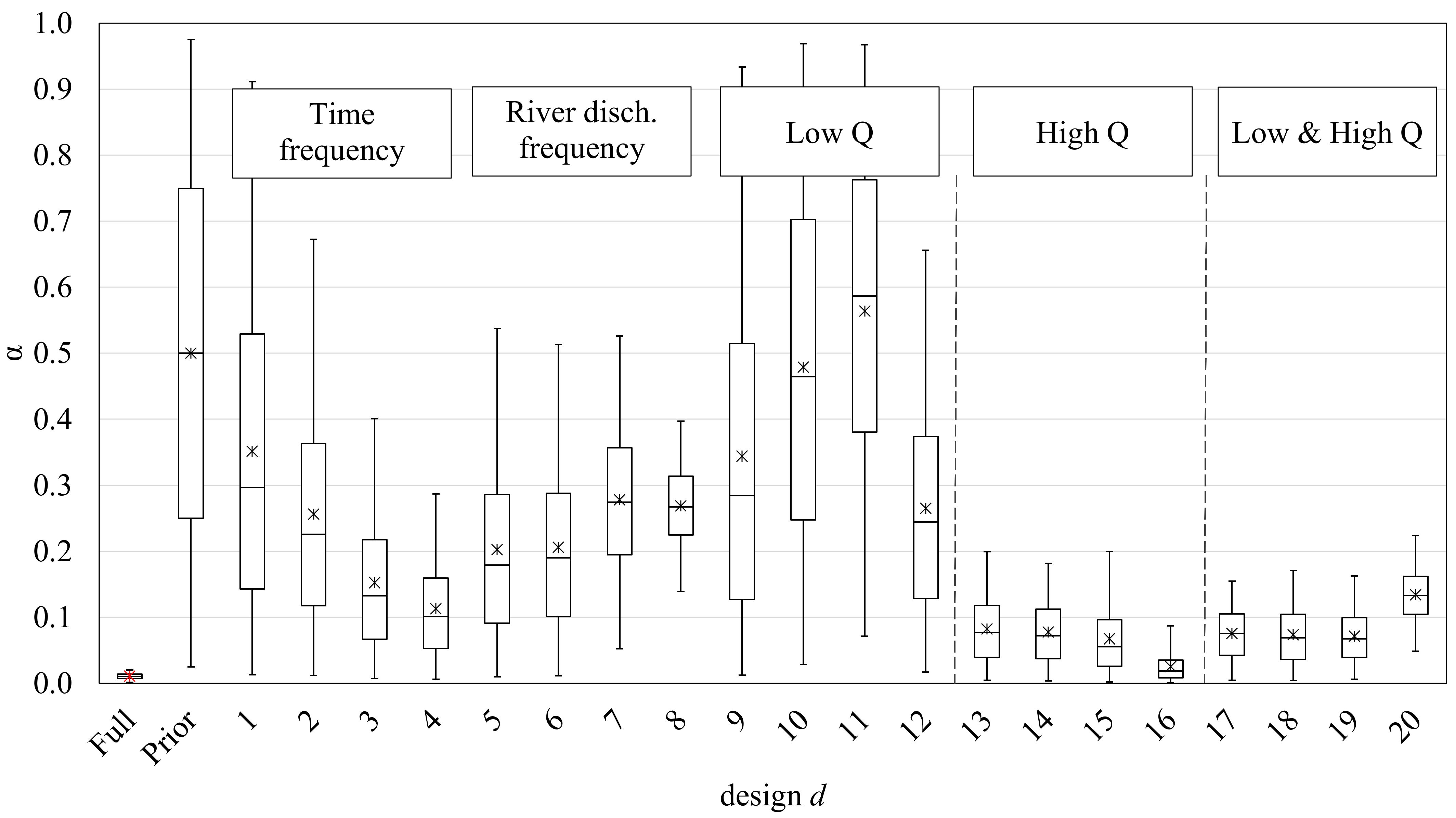
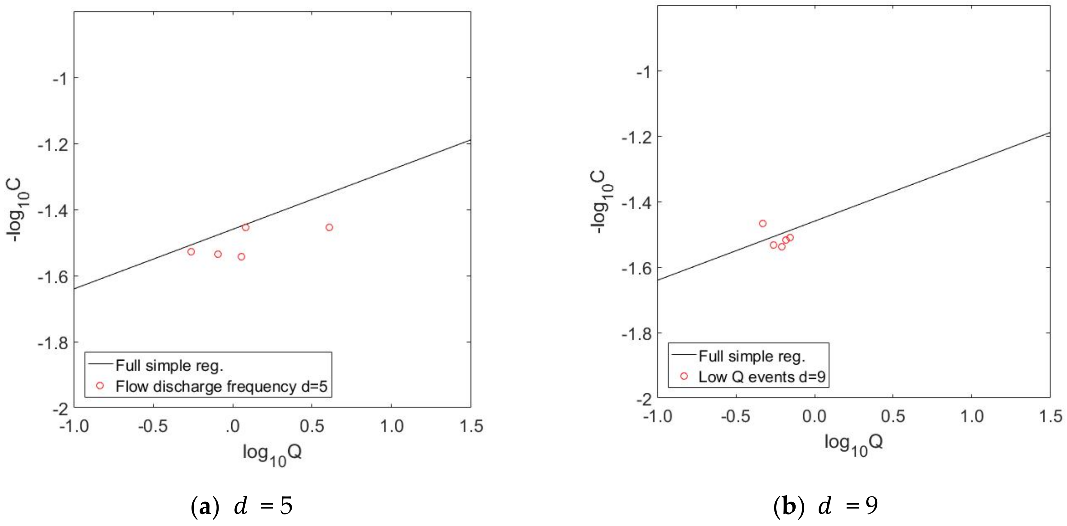
We propose 20 designs based on four sampling strategies (

Table 2. Sampling strategies.

d	Strategy	Description	# Samples
1	Time frequency	Samples are taken uniform in time: every 55 d	5
2		every 27.5 d	10
3		every 13.75 d	20
4		every 6.875 d	40
5	River discharge frequency	Samples are taken uniform in flow discharge: every 4,434,944 m3	5
6		every 2,217,472 m3	10
7		every 1,108,736m3	20
8		every 554,368 m3	40
9	Low Q	Samples are taken at low discharge rates (Q < 0.67 m3/s) that belong to different peak events (uncorrelated samples). We choose them equidistantly.	5
10			10
11			20
12			40
13	High Q	Samples are taken at high discharge rates (Q > 2.5 m3/s) for one peak event (correlated samples). When no more observations are available of one peak, we proceed to grab samples of a second peak event and so on.	5
14			10
15			20
16			40
17	Low and High Q	Samples are taken at low and high discharge rates following previous Low Q and High Q strategies. Half of the samples are at low Q except for d = 17 in which only two samples are at low Q.	5
18			10
19			20
20			40

). Firstly, we thinned out the observed data based on time-frequency strategies (d = 1 to 4). Secondly, we thinned out based on discharged volume within the river (d = 5 to 8). In both strategies, sampling was uniform (in time or discharged water), and we varied the number of samples between 5 and 40. Thirdly, we applied event-based sampling strategies, in which we considered samples at low discharge rates (d = 9 to 12) and high ones (d = 13–16). The last strategy considered low and high discharge rates together (d = 17 to 20). Here, we also considered between 5 and 40 samples. Designs should not be understood as random selections but manual selections as described in Appendix B. In this same appendix, the reader can find the observation values and the exact time coordinates for each sampling strategy.

For this study, we considered a low discharge rate to be lower than 0.67 m³/s (which corresponds to a value 25% below the mean discharge of the whole time series) and a high discharge rate to be Q > 2.5 m³/s.

3. Catchment and Data

The data used in this study were already published in 2013 [20]. The data were observed in the gauged catchment of the Ammer River located in the state of Baden-Württemberg in southwest Germany. The area of the catchment upstream of the gauging station Pfäffingen is 134 km². The geology is dominated by limestone of the Middle Triassic (“Oberer Muschelkalk”) and gypsum-bearing mudstone of the Upper Triassic (“Gipskeuper”). Both formations, particularly the limestone, are strongly karstified, and the Ammer River is primarily fed by karst springs, most of them being situated close to the main stem river [52]. In line with the large storage capacity of the karst system, the permeable rocks of the catchment lead to a dampened hydrologic variability with a very strong and steady baseflow. Mean annual low flow (0.44 m³/s) is as high as 50% of the long-term average flow (0.87 m³/s) (retrievable from https://www.hvz.baden-wuerttemberg.de/, accessed on 14 May 2020). Nevertheless, pronounced and sharp flood peaks typically occur during the summer season. They are caused by surface runoff generation on impervious urban areas in the upper catchment [20,53]. Usually, due to steep recessions, baseflow is attained within a few hours after the flood peaks. In total, 17% of the catchment area is urbanized and 71% is occupied by agriculture, 66% of which is used for arable land [20].

In terms of hydrochemistry, the strong and steady contribution from the limestone karst system leads to stable concentrations of geogenic and agriculture-derived solutes such as nitrate and chloride. A short-term dilution of these compounds may occur during storm events. Then, large amounts of event water with low solute content are introduced into the river [20]. Discharge data and chemical data were collected hourly with in situ analyzers from 07/1/2011 to 03/31/2012. This data set of observations includes over 6500 measurements of nitrate concentrations, electric conductivity, and discharge rates.

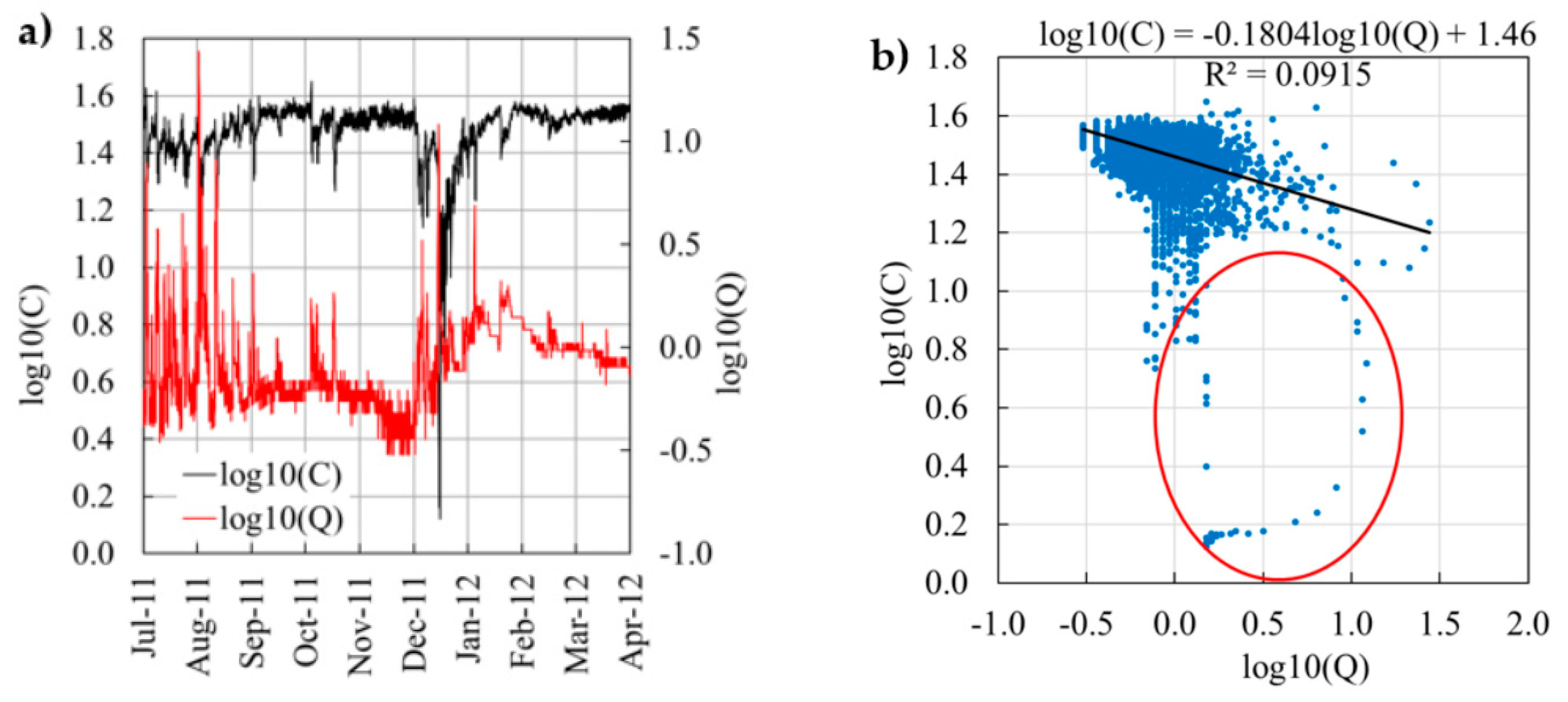
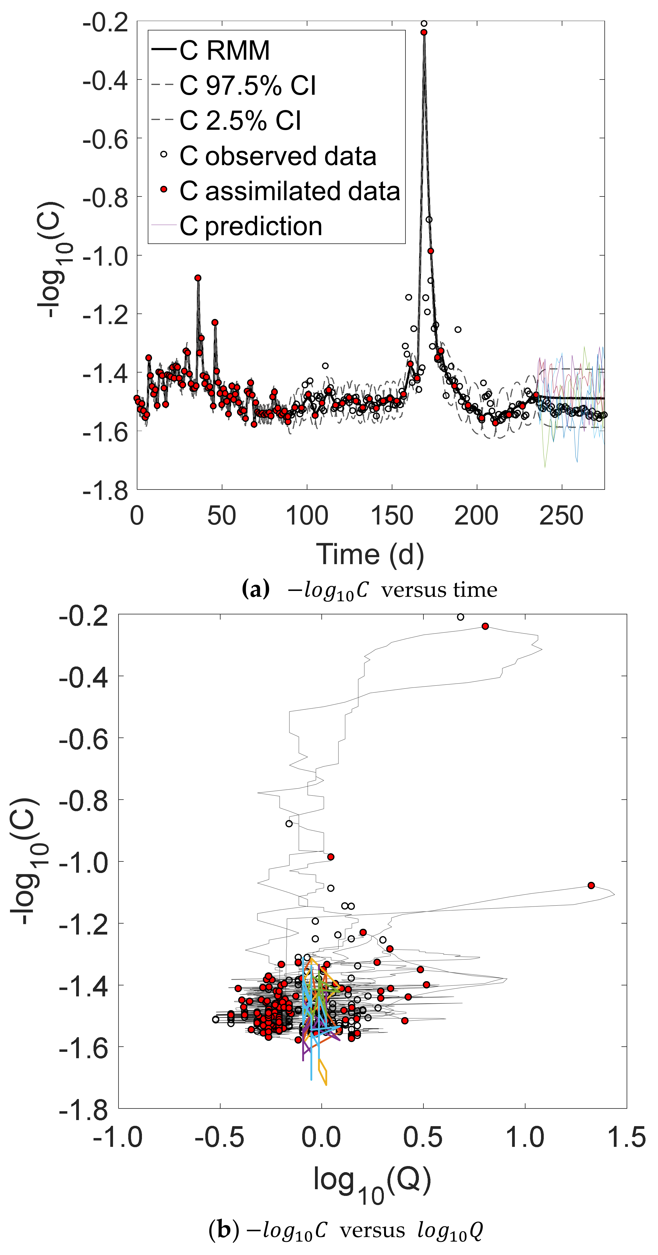
Here, we focus on discharge rate, Q, and nitrate concentration, C, (Figure 1a) although our proposed procedure could likewise be applied to other compounds. Over the time series, the average Q (0.93 m³/s) was similar to the long-term average (0.87 m³/s). The maximum Q (27.5 m³/s) represents an exceptional flood with a return period of about 20 years. The average C was 31.5 mg/L, but a range between 9.5 and 44.7 mg/L was captured.

Figure 1a demonstrates the strong baseflow component of the Ammer system with a steady Q and 60% of all measured values falling within the narrow range of 0.5–1.0 m³/s ($lo{g}_{10}Q$ = −0.30–0.00) during the recorded time series. During these baseflow periods, flow is predominantly fed from the large karst storage and, at rather constant rates, from wastewater treatment plant effluents, and thus exhibits stable nitrate concentrations around an average of 31.5 mg/L ($lo{g}_{10}C$ = 1.50). Most floods occur in the summer period and are the result of convective precipitation events. They typically have very short durations with steep recessions and cause a dilution of the nitrate concentrations. This may be explained by a fast runoff component dominated by a heavy precipitation event on sealed urban surfaces that carry low nitrate concentrations.

At the same time, flow supplied from the karst system with high C varies relatively little during flood events. There is no intermediate flow component that would connect agricultural soils with the stream network and mobilize additional nitrate fluxes. Such an interflow component would likely result in prolonged recessions of the hydrograph and, more importantly, positive relations between Q and C. In summary, the system is dominated by baseflow, which explains the clear tendency towards a chemostatic behavior.

Figure 1b shows the classic approach to determine the export regime of a catchment by computing a regression slope of $lo{g}_{10}C$ versus $lo{g}_{10}Q$. The effect of the short-term dilutions by event water inputs results in a slightly negative relation between Q and C, expressed by a small negative regression slope (−0.1804 in Figure 1b). This means that the Ammer River shows a rather chemostatic export regime for nitrate. The red circle in Figure 1b includes observations taken sequentially over time that belong to a hysteretic event. It depicts hysteresis in a highly visible fashion. Other hysteresis loops exist as well, e.g., the rightmost group of data points. Many more such loops are hidden in the bulk of the point cloud. With such unconventional residual statistics (i.e., loop patterns in the scatter around the regression line), the applied least-squares linear regression is not robust. Especially for smaller time series, almost any regression slope between 0 and −1 (and even outside these bounds) would be possible.

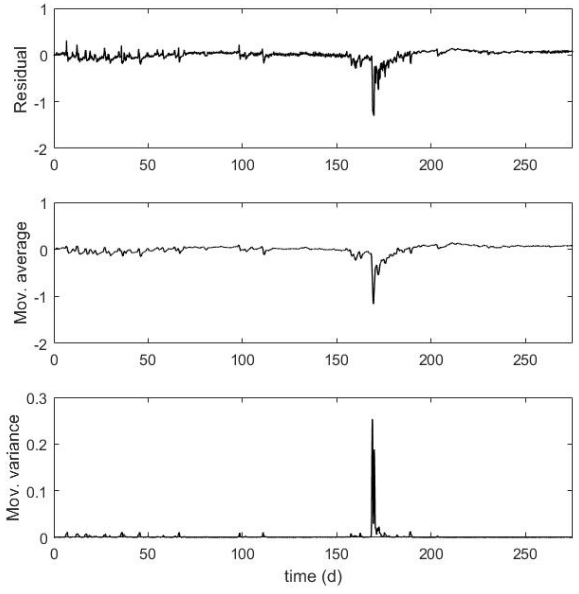
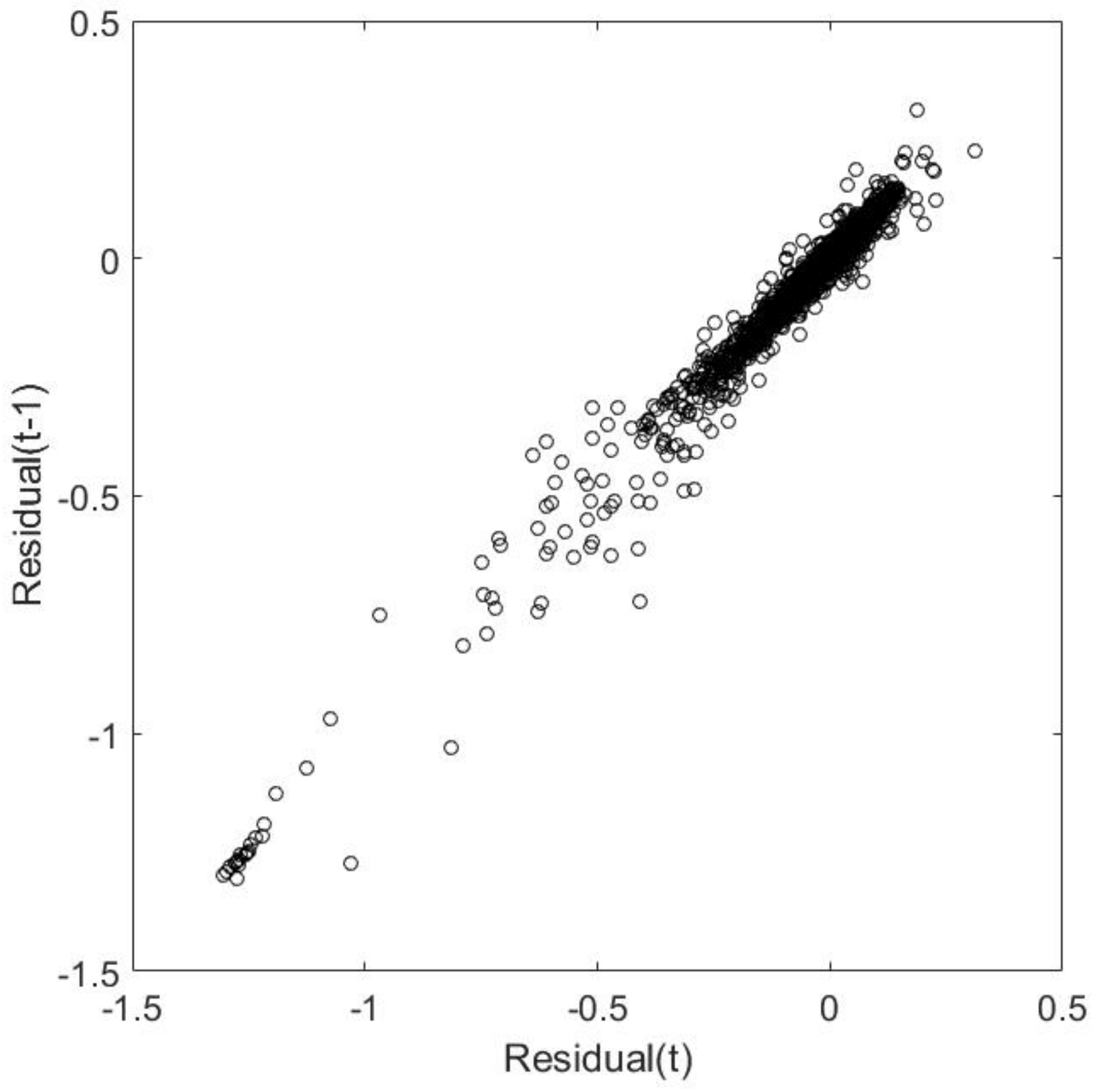
To show that these data do not comply with the regression assumptions (e.g., the mean is not constantly zero and the variance is not constant), we computed the residuals in the C–Q regression of the Ammer catchment. In Appendix A, we present the plots of the residuals, moving window average, and moving window variance (Figure A1), as well as the correlation of Residual(t) with Residual(t-1) (Figure A2).

4. Results

4.1. RMM Simulations

Figure 2 displays some examples generated with our RMM for a fixed hyper-parameter (α or t_ch), while the other three parameters are inferred by Bayesian inference using the full-time series data.

Table 3. Inferred hyper-parameters values when α or t_ch are fixed using the full time-series data.

	Fixed Hyper-Parameter
	α = 0	α = 1	tch = 20	tch = 500
	Inferred Hyper-Parameter
α (/)	-	-	0.218	0.016
tch (h)	105.9	42.1	-	-
$m_k$$\left(\frac{mg}{l}{\left(\frac{m^3}{h}\right)}^{\alpha }\right)$	31.0	23.6	27.1	17.5
$\sqrt{v_k}$$\left(\frac{mg}{l}{\left(\frac{m^3}{h}\right)}^{\alpha }\right)$	7.0	28.3	1.9	39.8

includes the inferred hyper-parameters used to generate the concentration time series shown in Figure 2.

Figure 2a shows $-lo{g}_{10}C$ versus time for the two fixed values of $\alpha$ (0 and 1) and the two fixed values of $t_{ch}$ (20 h and 500 h), whereas Figure 2b shows $-lo{g}_{10}C$ versus $lo{g}_{10}Q$ for the same fixed values of $\alpha$ and $t_{ch}$. Observing the different patterns of $\alpha$ from 0 (blue) to 1 (red), and of $t_{ch}$ from 20 h (orange) to 500 h (purple), it can be seen that greater values of $\alpha$ and $t_{ch}$ produce larger changes in the concentration values. Figure 2b shows how our model is able to reproduce the hysteresis phenomena with the presence of loops.

We would like to mention that the CPU time of applying our RMM model together with MCMC (for an ensemble size of 100,000) is less than three minutes on a standard desktop PC (Intel^® Core™ i7-7700 CP @3.60 GHz, 32 GB of RAM), which makes it a very affordable and efficient model.

4.2. Characterization with Extensive Time-Series Data

In

Table 4. Inferred values of the Ammer catchment using the whole time-series data (a total of 6604 measurements).

Parameter (Unit)	Inferred Value
${\alpha }_{full}$ (/)	0.011
$t_{ch,full}$ (h)	106.4
$m_{k,full}$$\left(\frac{mg}{l}{\left(\frac{m^3}{h}\right)}^{\alpha }\right)$	30.8
$\sqrt{v_{k,full}}$$\left(\frac{mg}{l}{\left(\frac{m^3}{h}\right)}^{\alpha }\right)$	2.6

, we show the inferred mean posterior values of $\alpha$, $t_{ch}$, $m_k$, and $v_k$ based on the full given discharge data $Q_t$ and measured concentration data $C_t$.

The referral value for ${\alpha }_{full}$ is equal to 0.011 and corresponds to a chemostatic behavior (γ ≈ 0). Therefore, concentration mainly depends on the apparent release rate $k$ (Equation (1)). This agrees with the hydrochemical arguments by Schwientek et al. [20] discussed in Section 3. $t_{ch,full}$ is equal to 106.4 h, which corresponds to 4.4 days. This value is similar to the assumed mean of four days in Table 1. Therefore, the Ammer river indeed presents roughly weekly cycles of nitrate concentration release into the river.

The average expected nitrate concentration is $m_{k,full}$ = 30.8, which lies between pristine water (1 mg/L) and the integral catchment output during baseflow (Section 2.2.1). Also, $m_{k,full}$ is very similar to the average $C$ (31.5 mg/L) obtained in Schwientek et al. [20]. The variance of $k$ is $v_{k,full}$ = 7.83, which indicates that the system has a relatively low dynamic in (log-)release.

Figure 3 shows that the interpolation (black line) produced by the RMM, when applying inferred values in Table 4, fully goes through the data we used for calibration (red points). This figure also displays the credible intervals (CI) (2.5% and 97.5%, respectively) for daily observations (time = 0–90 days), every 4 days (time = 90–180 days), every 8 days (time = 180–240 days), and no sampling (time > 240 days). The 95% range is more narrow when more observations are considered, decreasing the uncertainty of the RMM interpolation. Thus, the RMM cannot only calibrate the hyper-parameters of the actual time series, but can also interpolate with quantified standard errors (grey lines). Figure 3 also shows some concentration predictions (colored lines) generated by the RMM after the calibration.

4.3. Characterization with Sparse Data (Sampling Strategies)

Figure 4 shows the prior and posterior distributions of $\alpha$ for the sampling strategies described in Table 2. The minimum and maximum of the box plots mark the 95% CI (2.5% and 97.5% values, respectively). The red star marks the posterior mean of ${\alpha }_{full}$, whereas the black stars mark the posterior mean values inferred by the designs. Only design $d$ = 16 can reproduce a posterior $\alpha$ with very high confidence. Yet, the other event-based designs involving samples at high $Q$ (High $Q$ events $d$ = 13 to 16, and Low and High $Q$ events $d$ = 17 to 20) are surprisingly confident, although using only very few samples. All these strategies present a range of the 95% CI lower than 0.200 (

Table 5. Summary of α and range of CI 95% for each design for the RMM and linear regression model after applying ODE. Highlighted in green and grey are the best and worst sampling strategies of the RMM, respectively.

			RMM				Linear Regression
	d	# Samples	${\alpha }_{full}$	CI 2.5%	CI 97.5%	Range 95%	${\alpha }_{reg}$	CI 2.5%	CI 97.5%	Range 95%
	Full	6604	0.011	0.002	0.02	0.018	0.180	0.167	0.194	0.027
	Prior	0	0.5	0.025	0.950	0.950
	d	# samples	${\alpha }_{post,d}$	CI 2.5%	CI 97.5%	Range 95%	${\alpha }_{reg,d}$	CI 2.5%	CI 97.5%	Range 95%
Time frequency	1	5	0.351	0.013	0.911	0.898	−0.093	−0.696	0.509	1.206
	2	10	0.256	0.012	0.673	0.661	0.119	−0.095	0.333	0.429
	3	20	0.153	0.008	0.401	0.393	0.109	−0.073	0.291	0.364
	4	40	0.113	0.006	0.287	0.281	0.055	−0.144	0.253	0.397
River discharge frequency	5	5	0.202	0.01	0.537	0.527	0.094	−0.087	0.275	0.363
	6	10	0.206	0.011	0.513	0.502	0.131	−0.035	0.298	0.333
	7	20	0.278	0.052	0.526	0.474	0.259	0.041	0.477	0.436
	8	40	0.269	0.139	0.397	0.258	0.262	0.141	0.383	0.243
Low Q	9	5	0.344	0.012	0.934	0.922	−0.242	−0.832	0.348	1.180
	10	10	0.479	0.028	0.969	0.941	0.981	−1.080	3.041	4.121
	11	20	0.564	0.072	0.967	0.896	0.550	−0.380	1.480	1.860
	12	40	0.265	0.017	0.656	0.64	0.311	−0.175	0.796	0.971
High Q	13	5	0.083	0.005	0.200	0.195	0.208	−0.264	0.679	0.943
	14	10	0.078	0.003	0.182	0.178	0.117	−0.251	0.484	0.735
	15	20	0.067	0.002	0.200	0.198	0.103	−0.094	0.300	0.394
	16	40	0.025	0.001	0.087	0.086	0.020	−0.447	0.488	0.935
Low & High Q	17	5	0.076	0.005	0.155	0.15	0.040	−0.045	0.126	0.171
	18	10	0.074	0.004	0.171	0.167	0.102	0.020	0.184	0.163
	19	20	0.072	0.006	0.163	0.156	0.164	0.097	0.232	0.135
	20	40	0.134	0.049	0.224	0.175	0.227	0.176	0.278	0.102

).

Table 5 summarizes the results of the 20 sampling strategies for the RMM, including posterior alpha ${\alpha }_{post,d}$ (Equation (16)), the value of the 95% range, and values of the 2.5% CI and 97.5% CI.

Generally, increasing the number of samples from 5 to 40 decreases the bias of the posterior mean ${\alpha }_{post,d}$. It also increases the reliability of the designs: the range of the CI decreases. For instance, the time frequency strategy produces a quick reduction of the $\alpha$ bias when the number of samples increases: ${\alpha }_{post,d}$ decreases from 0.351 ($d$ = 1 with five samples) to 0.113 ($d$ = 4 with 40 samples). In addition, the width of the 95% range for $d$ = 4 is reduced from the prior value of 0.95 (0.975–0.025) to 0.28 (0.29–0.01). However, strategies based on river discharge frequency and Low $Q$ events do not follow this tendency; instead, their biases of ${\alpha }_{post,d}$ seem to increase when increasing the number of samples from 5 to 20 (e.g., $d$ = 5 versus $d$ = 7). However, these two types of strategies seem to benefit when the number of samples is increased to 40 (see Section 5.3). Therefore, an improvement will be expected when more samples are taken for these two types of strategies.

As already mentioned, when we apply sampling strategies based on events (Figure 4), we can observe two different performances. There are sampling strategies that decrease the bias and uncertainty of ${\alpha }_{post,d}$ significantly, such as strategies based on High $Q$ events ($d$ = 13 to 16) and Low and High $Q$ events ($d$ = 17 to 20). All these strategies have a ${\alpha }_{post,d}$ between 0.025 and 0.134. On the other hand, the sampling strategy only based on Low $Q$ events show a low bias reduction when taking 40 samples ($d$ = 12), showing ${\alpha }_{post,d}=$ 0.265. Thus, we have strong and weak event-based sampling strategies.

Strategies that show the lowest reduction of uncertainty (when range CI 95% > 0.50) include both strategies based on frequency for a low number of samples (5 and 10, $d$ = 1,2, 5, and 6) and strategies based on measuring Low $Q$ events ($d$ = 9 to 12). Obviously, strategies with only 5 or 10 samples involve less information; therefore, a slight improvement of the posterior is expected. However, as observed in Figure 4 and Table 5, strategies that collect data during High $Q$ events even with a low number of samples produce a significant reduction of the bias and uncertainty of ${\alpha }_{post}$.

In summary, from the five types of strategies (Figure 4), the High $Q$ events strategy stands out as the best strategy because it not only decreases the posterior bias, but also reduces the uncertainty width. Another good option that improves the prediction of ${\alpha }_{post}$ is applying the Low and High $Q$ events strategy, although it presents a higher bias and uncertainty. Therefore, to maximize the variance reduction of the export strength and minimize the data collection cost, we recommend High $Q$ events strategies.

5. Discussion

5.1. Comparison of the RMM to the Linear Regression Approach

Both methods, namely RMM and linear regression, agreed that the Ammer catchment shows a chemostatic regime with ${\alpha }_{full}$ = 0.011 and ${\alpha }_{reg}$ = 0.180, respectively, when all 6604 samples were used for the analysis. However, we strongly believe that, with much fewer data used, ${\alpha }_{post,d}$ inferred with our method is more robust than ${\alpha }_{reg,d}$ obtained by simple regression. Table 5 also includes a summary of ${\alpha }_{reg,d}$ produced by simple regression when applying the different sampling strategies in Table 2. While the 95% CI for the RMM is based on the likelihood-weighted MCMC results, the 95% CI for the regression slope is taken from the standard textbook equation, as in [31].

Our method shows robustness: ${\alpha }_{post,d}$ decreases, approaching the inferred value, when increasing the number of samples. In addition, when increasing the number of samples, the width of the confidence range decreases. On the other hand, ${\alpha }_{reg,d}$ can show negative values for some sampling strategies or even values greater than one. These negative ${\alpha }_{reg,d}$ do not make any sense since $\alpha$ should always be within the interval [0,1] for the Ammer catchment; thus ${\alpha }_{reg,d}$ shows a much larger impact of randomness. For example, when we increase the number of samples, for $d$ = 1 to $d$ = 2 and $d$ = 3, ${\alpha }_{reg,d}$ increases and decreases inconsistently.

Interestingly, designs $d$ = 4 and $d$ = 16 produce ${\alpha }_{reg,d}$ close to ${\alpha }_{full}$, which is probably a consequence of the high number of samples ($d$ = 4 time frequency with 40 samples) and a consequence of choosing a suitable sampling strategy based on high discharge rates ($d$ = 16 High $Q$ events with 40 samples).

To summarize, we have shown that the simple regression approach can be misleading for small, economically efficient sampling campaigns. We have also shown the strongly increased robustness of our model compared to conventional regression. Therefore, the results of this study can help characterize the export regime of a catchment and manage water pollution in rivers at lower monitoring costs.

5.2. Performance of Sampling Strategies

Figure 5 shows plots of $-lo{g}_{10}C$ versus $lo{g}_{10}Q$ for event-based designs with 40 samples ($d=$ 12, 16, and 20). For each design, we show the slope produced by linear regression ${\alpha }_{reg}$= 0.180 (black line) and the observed values (red circles).

Strategies based on Low Q events show a low performance (Section 4.3) because they cover small ranges of $C$ and $Q$ (Figure 5a). As already seen in Section 4.3, the best strategies involve sampling during one or more peak events or several events of low discharge. However, the designs based on Low and High $Q$ events present a larger uncertainty than designs based only on High $Q$ events. Measuring during large peak events (High $Q$ events strategy) ensures that data include changes of $C$ when $Q$ increases and decreases (loops seen in Figure 5b,c on the right side). Measuring at low and high events also allows for a wide range of $Q$ values (Figure 5c).

On the other hand, the worst strategies with a higher bias of ${\alpha }_{post}$ are based on river discharge frequency and on measuring events at low $Q$. Therefore, combinations of samples belonging to different flood events (e.g., $d$ = 5, 6, and 7, i.e., when the number of samples is between 5 and 20 for river discharge frequency) do not produce a good ${\alpha }_{post,d}$, since the valuable information of the memory-type relationship between $Q$ and $C$ is missing. Figure 6a displays $d$ = 5 (river discharge frequency with five samples) and Figure 6b shows $d$ = 9 (low Q events with five samples). Figure 6 clearly shows that five samples are not enough to catch loop changes of $C–Q$ or cover a wide range of $Q$.

When only Low $Q$ events are measured ($d$ = 9 to 12), the strategy fails to span a range of different $Q$ values even when the number of samples is increased to 40; therefore, they do not produce good posteriors. Thus, some sampling strategies improve by increasing the number of observations, but others will not benefit.

In summary, we have shown that sampling strategies based on extreme events (including High Q or both High and Low Q) are key to inferring the catchment behavior with low bias and low uncertainty. This is important, regardless of whether using our RMM or linear regression.

5.3. Comparison to Other Studies

The idea that the perceived C–Q relationship changes when samples are taken by time frequency or by events is not new. Recent studies have distinguished between low and high discharge rates to determine C–Q relationships [5,6,22,36,40], and others have looked at the frequency of sampling [14,22] or sampling strategy [34].

Minaudo et al. [40] created a model in which C is subject to slow Q (seasonal) and fast Q (storm event) variations. Knapp et al. [5] showed that the C–Q relationship differed significantly for some solutes (NO₃, K, Cl) depending on when samples were observed. The C–Q relationship of these solutes was differently impacted when discharge changes were caused by individual peak events or by longer time scales. These studies observed opposite export regimes based on when measurements were observed. Contrarily, the RMM shows robustness (Table 5) since it does not result in “opposite” export regimes depending on when samples are taken.

Floury et al. [14] evaluated the effects of lowering the sampling frequency on the hydrochemical signal by applying artificial subsampling to the high-frequency sampling. They found that concentration signals were degraded by being smoothed. Bieroza et al. [11] showed that a lower number of samples produced more uncertainty in water quality parameters as a function of the C–Q slope. In our study, we observed the same trend. However, our RMM can predict a good export regime with only five samples if the sampling strategy is based on High Q events (d = 13). Nevertheless, the prediction notably improves when the number of samples increases.

Zhang and Ball [34] tested different sampling approaches and used various models (including the WRTDS model). Their best strategy included a mixture of 12 regular samples and 8 stormflow samples per year. However, they did not consider a sampling strategy that only accounted for High Q events. The finding that sampling at High Q events is better informs concentration pattern evolution with discharge was expected. At baseflow, nitrate concentrations remain quite constant; the information added by sampling again at low discharges is low. In contrast, at high discharges, where nitrate concentrations evolve the most, adding another sample is valuable to characterize the concentration variation with discharge.

6. Summary and Conclusions

In this work, we proposed a better and more robust alternative to model the behavior of a catchment. Generally, the export regime of a catchment (chemostatic, dilution, or mobilization type) is characterized by the slope obtained by plotting $lo{g}_{10}C$ versus $lo{g}_{10}Q$ measured in the river at the catchment outlet. However, we can usually observe in this representation that measurements show hysteresis effects of the system, defying the assumptions of linear regression. With these assumptions violated, linear regression results can be suboptimal, biased, and strongly misleading. In contrast, our regime-and-memory model (RMM) includes an explicit parameter to model the type of export regime and a parameter to account for the characteristic time scale of release and chemical turnover in the catchment. Thus, our model can mimic these memory effects of the catchment.

For demonstration, we used a high-frequency data series of nitrate concentrations collected with a high-frequency in situ analyzer in a catchment in Germany for nine months. We showed that our simple model is able to mimic the nitrate dynamics of the catchment, including the hysteresis effect. Also, our model showed robustness and consistency in inferring the export regime compared to the linear regression, even for much smaller data sets. Thus, our RMM has the potential to improve export regime predictions.

Regarding the sampling strategies, we found out that the strongest sampling strategies are based on High Q events for the Ammer catchment. These strategies cover a large range of discharge rates and accompanied C values. Representativeness of the collected data (in the face of short-term fluctuations in compound release and catchment memory effects) is ensured by stretching the sampling days across events. From our analyses, we observed that five samples/observations are necessary to produce a significant reduction of α bias (or better accuracy) if the right sampling strategy is implemented (High Q events strategy). However, to decrease the uncertainty (or increase the precision), one must increase the number of samples.

Thus, for catchments with similar characteristics to the Ammer catchment, we recommend collecting the samples when peak events occur since this provides a wide range of Q in a short time interval. However, it bears the risk that these large events are dependent on the season, so their observation would be restricted seasonally. To avoid this seasonal restriction, alternatively, we recommend measuring samples at uncorrelated events at low Q. However, the uncertainty of the export regime will be larger than when C is measured only at High Q events. Hence, sampling strategies based on extreme events, both at low and high Q, are key to reducing the prediction uncertainty of the catchment behavior, and event-based thinking can be reasonably generalized to catchments with C–Q behavior that can be represented by our RMM.

Future work with the RMM includes validating these statements with longer time series, more solutes, as well as data from different catchments. Also, further research will be needed to extend the presented statistical approach of the RMM to consider $\alpha$ for the mobilization transport regime (for positive correlations of $lo{g}_{10}Q$ versus $lo{g}_{10}C$), in which wet periods do not result in dilution but an additional mobilization of substances.

References

1. Basu, N.B.; Destouni, G.; Jawitz, J.W.; Thompson, S.E.; Loukinova, N.V.; Darracq, A.; Zanardo, S.; Yaeger, M.; Sivapalan, M.; Rinaldo, A.; et al. Nutrient loads exported from managed catchments reveal emergent biogeochemical stationarity. Geophys. Res. Lett. 2010, 37, L23404. [Google Scholar] [CrossRef]
2. Basu, N.B.; Thompson, S.E.; Rao, P.S.C. Hydrologic and biogeochemical functioning of intensively managed catchments: A synthesis of top-down analyses. Water Resour. Res. 2011, 47. [Google Scholar] [CrossRef] [Green Version]
3. Dupas, R.; Minaudo, C.; Abbott, B.W. Stability of spatial patterns in water chemistry across temperate ecoregions. Environ. Res. Lett. 2019, 14, 074015. [Google Scholar] [CrossRef] [Green Version]
4. Godsey, S.E.; Kirchner, J.W.; Clow, D.W. Concentration–discharge relationships reflect chemostatic characteristics of US catchments. Hydrol. Process. 2009, 23, 1844–1864. [Google Scholar] [CrossRef]
5. Knapp, J.; Freiin von Freyberg, J.; Studer, B.; Kiewiet, L.; Kirchner, J.W. Concentration-discharge relationships vary among hydrological events, reflecting differences in event characteristics. Hydrol. Earth Syst. Sci. Discuss. 2020, 24, 2561–2576. [Google Scholar] [CrossRef]
6. Moatar, F.; Abbott, B.W.; Minaudo, C.; Curie, F.; Pinay, G. Elemental properties, hydrology, and biology interact to shape concentration-discharge curves for carbon, nutrients, sediment, and major ions. Water Resour. Res. 2017, 53, 1270–1287. [Google Scholar] [CrossRef]
7. Musolff, A.; Schmidt, C.; Selle, B.; Fleckenstein, J.H. Catchment controls on solute export. Adv. Water Resour. 2015, 86, 133–146. [Google Scholar] [CrossRef]
8. Clow, D.W.; Drever, J.I. Weathering rates as a function of flow through an alpine soil. Chem. Geol. 1996, 132, 131–141. [Google Scholar] [CrossRef]
9. Godsey, S.E.; Hartmann, J.; Kirchner, J.W. Catchment chemostasis revisited: Water quality responds differently to variations in weather and climate. Hydrol. Process. 2019, 33, 3056–3069. [Google Scholar] [CrossRef]
10. Rode, M.; Wade, A.J.; Cohen, M.J.; Hensley, R.T.; Bowes, M.J.; Kirchner, J.W.; Arhonditsis, G.B.; Jordan, P.; Kronvang, B.; Halliday, S.J.; et al. Sensors in the stream: The high-frequency wave of the present. Environ. Sci. Technol. 2016, 50, 10297–10307. [Google Scholar] [CrossRef] [Green Version]
11. Bieroza, M.Z.; Heathwaite, A.L.; Bechmann, M.; Kyllmar, K.; Jordan, P. The concentration-discharge slope as a tool for water quality management. Sci. Total Environ. 2018, 630, 738–749. [Google Scholar] [CrossRef] [Green Version]
12. Bowes, M.J.; Jarvie, H.P.; Halliday, S.J.; Skeffington, R.A.; Wade, A.J.; Loewenthal, M.; Gozzard, E.; Newman, J.R.; Palmer-Felgate, E.J. Characterising phosphorus and nitrate inputs to a rural river using high-frequency concentration–flow relationships. Sci. Total Environ. 2015, 511, 608–620. [Google Scholar] [CrossRef] [PubMed] [Green Version]
13. Evans, C.; Davies, T.D. Causes of concentration/discharge hysteresis and its potential as a tool for analysis of episode hydrochemistry. Water Resour. Res. 1998, 34, 129–137. [Google Scholar] [CrossRef]
14. Floury, P.; Gaillardet, J.; Gayer, E.; Bouchez, J.; Tallec, G.; Ansart, P.; Koch, F.; Gorge, C.; Blanchouin, A.; Roubaty, J.-L. The potamochemical symphony: New progress in the high-frequency acquisition of stream chemical data. Hydrol. Earth Syst. Sci. 2017, 21, 6153–6165. [Google Scholar] [CrossRef] [Green Version]
15. Grimaldi, C.; Grimaldi, M.; Millet, A.; Bariac, T.; Boulègue, J. Behaviour of chemical solutes during a storm in a rainforested headwater catchment. Hydrol. Process. 2004, 18, 93–106. [Google Scholar] [CrossRef]
16. Jones, T.D.; Chappell, N.A.; Tych, W. First dynamic model of dissolved organic carbon derived directly from high-frequency observations through contiguous storms. Environ. Sci. Technol. 2014, 48, 13289–13297. [Google Scholar] [CrossRef] [PubMed]
17. Liu, W.; Youssef, M.A.; Birgand, F.P.; Chescheir, G.M.; Tian, S.; Maxwell, B.M. Processes and mechanisms controlling nitrate dynamics in an artificially drained field: Insights from high-frequency water quality measurements. Agric. Water Manag. 2020, 232, 106032. [Google Scholar] [CrossRef]
18. Ockenden, M.; Tych, W.; Beven, K.; Collins, A.; Evans, R.; Falloon, P.; Forber, K.; Hiscock, K.; Hollaway, M.; Kahana, R.; et al. Prediction of storm transfers and annual loads with data-based mechanistic models using high-frequency data. Hydrol. Earth Syst. Sci. 2017, 6425–6444. [Google Scholar] [CrossRef] [Green Version]
19. Rusjan, S.; Brilly, M.; Mikoš, M. Flushing of Nitrate from a Forested Watershed: An Insight into hydrological nitrate mobilization mechanisms through seasonal high-frequency stream nitrate dynamics. J. Hydrol. 2008, 354, 187–202. [Google Scholar] [CrossRef]
20. Schwientek, M.; Osenbrück, K.; Fleischer, M. Investigating hydrological drivers of nitrate export dynamics in two agricultural catchments in Germany using high-frequency data series. Environ. Earth Sci. 2013, 69, 381–393. [Google Scholar] [CrossRef]
21. Abbott, B.W.; Gruau, G.; Zarnetske, J.P.; Moatar, F.; Barbe, L.; Thomas, Z.; Fovet, O.; Kolbe, T.; Gu, S.; Pierson-Wickmann, A.-C.; et al. Unexpected spatial stability of water chemistry in headwater stream networks. Ecol. Lett. 2018, 21, 296–308. [Google Scholar] [CrossRef]
22. Bieroza, M.Z.; Heathwaite, A.L. Seasonal variation in phosphorus concentration–discharge hysteresis inferred from high-frequency in situ monitoring. J. Hydrol. 2015, 524, 333–347. [Google Scholar] [CrossRef] [Green Version]
23. Dupas, R.; Gascuel-Odoux, C.; Gilliet, N.; Grimaldi, C.; Gruau, G. Distinct export dynamics for dissolved and particulate phosphorus reveal independent transport mechanisms in an arable headwater catchment. Hydrol. Process. 2015, 29, 3162–3178. [Google Scholar] [CrossRef]
24. Hornberger, G.M.; Scanlon, T.M.; Raffensperger, J.P. Modelling transport of dissolved silica in a forested headwater catchment: The effect of hydrological and chemical time scales on hysteresis in the concentration–discharge relationship. Hydrol. Process. 2001, 15, 2029–2038. [Google Scholar] [CrossRef]
25. House, W.A.; Warwick, M.S. Hysteresis of the solute concentration/discharge relationship in rivers during storms. Water Res. 1998, 32, 2279–2290. [Google Scholar] [CrossRef]
26. Rose, L.A.; Karwan, D.L.; Godsey, S.E. Concentration–discharge relationships describe solute and sediment mobilization, reaction, and transport at event and longer timescales. Hydrol. Process. 2018, 32, 2829–2844. [Google Scholar] [CrossRef]
27. Butturini, A.; Alvarez, M.; Bernal, S.; Vazquez, E.; Sabater, F. Diversity and temporal sequences of forms of DOC and NO3-discharge responses in an intermittent stream: Predictable or random succession? J. Geophys. Res. Biogeosci. 2008, 113. [Google Scholar] [CrossRef]
28. Langlois, J.L.; Johnson, D.W.; Mehuys, G.R. Suspended sediment dynamics associated with snowmelt runoff in a small mountain stream of Lake Tahoe (Nevada). Hydrol. Process. 2005, 19, 3569–3580. [Google Scholar] [CrossRef]
29. Lawler, D.M.; Petts, G.E.; Foster, I.D.L.; Harper, S. Turbidity dynamics during spring storm events in an urban headwater river system: The upper tame, West Midlands, UK. Sci. Total Environ. 2006, 360, 109–126. [Google Scholar] [CrossRef]
30. Lloyd, C.E.M.; Freer, J.E.; Johnes, P.J.; Collins, A.L. Using hysteresis analysis of high-resolution water quality monitoring data, including uncertainty, to infer controls on nutrient and sediment transfer in catchments. Sci. Total Environ. 2016, 543, 388–404. [Google Scholar] [CrossRef] [Green Version]
31. Chatterjee, S.; Hadi, A.S. Regression Analysis by Example; John Wiley & Sons: Hoboken, NJ, USA, 2015; ISBN 978-1-119-12273-9. [Google Scholar]
32. Hirsch, R.M.; Moyer, D.L.; Archfield, S.A. Weighted regressions on time, discharge, and season (WRTDS), with an application to chesapeake bay river inputs1. JAWRA J. Am. Water Resour. Assoc. 2010, 46, 857–880. [Google Scholar] [CrossRef]
33. Zhang, Q.; Harman, C.J.; Ball, W.P. An improved method for interpretation of riverine concentration-discharge relationships indicates long-term shifts in reservoir sediment trapping. Geophys. Res. Lett. 2016, 43, 10215–10224. [Google Scholar] [CrossRef]
34. Zhang, Q.; Ball, W.P. Improving riverine constituent concentration and flux estimation by accounting for antecedent discharge conditions. J. Hydrol. 2017, 547, 387–402. [Google Scholar] [CrossRef] [Green Version]
35. Tunqui Neira, J.M.; Andréassian, V.; Tallec, G.; Mouchel, J.-M. Technical note: A two-sided affine power scaling relationship to represent the concentration–discharge relationship. Hydrol. Earth Syst. Sci. 2020, 24, 1823–1830. [Google Scholar] [CrossRef] [Green Version]
36. Underwood, K.L.; Rizzo, D.M.; Schroth, A.W.; Dewoolkar, M.M. Evaluating spatial variability in sediment and phosphorus concentration-discharge relationships using bayesian inference and self-organizing maps. Water Resour. Res. 2017, 53, 10293–10316. [Google Scholar] [CrossRef] [Green Version]
37. Qian, S.S.; Reckhow, K.H.; Zhai, J.; McMahon, G. Nonlinear regression modeling of nutrient loads in streams: A bayesian approach. Water Resour. Res. 2005, 41. [Google Scholar] [CrossRef] [Green Version]
38. Blaen, P.J.; Khamis, K.; Lloyd, C.E.M.; Bradley, C.; Hannah, D.; Krause, S. Real-time monitoring of nutrients and dissolved organic matter in rivers: Capturing event dynamics, technological opportunities and future directions. Sci. Total Environ. 2016, 569–570, 647–660. [Google Scholar] [CrossRef] [Green Version]
39. Jachens, E.R.; Rupp, D.E.; Roques, C.; Selker, J.S. Recession analysis revisited: Impacts of climate on parameter estimation. Hydrol. Earth Syst. Sci. 2020, 24, 1159–1170. [Google Scholar] [CrossRef] [Green Version]
40. Minaudo, C.; Dupas, R.; Gascuel-Odoux, C.; Roubeix, V.; Danis, P.-A.; Moatar, F. Seasonal and event-based concentration-discharge relationships to identify catchment controls on nutrient export regimes. Adv. Water Resour. 2019, 131, 103379. [Google Scholar] [CrossRef]
41. Shogren, A.J.; Zarnetske, J.P.; Abbott, B.W.; Iannucci, F.; Bowden, W.B. We cannot shrug off the shoulder seasons: Addressing knowledge and data gaps in an arctic headwater. Environ. Res. Lett. 2020. [Google Scholar] [CrossRef]
42. Yoon, B.; Raymond, P.A. Dissolved organic matter export from a forested watershed during Hurricane Irene. Geophys. Res. Lett. 2012, 39. [Google Scholar] [CrossRef]
43. Zimmer, M.A.; Pellerin, B.; Burns, D.A.; Petrochenkov, G. Temporal variability in nitrate-discharge relationships in large rivers as revealed by high-frequency data. Water Resour. Res. 2019, 55, 973–989. [Google Scholar] [CrossRef]
44. Thomas, Z.; Abbott, B.W.; Troccaz, O.; Baudry, J.; Pinay, G. Proximate and ultimate controls on carbon and nutrient dynamics of small agricultural catchments. Biogeosciences 2016, 13, 1863–1875. [Google Scholar] [CrossRef] [Green Version]
45. Diggle, P.; Lophaven, S. Bayesian geostatistical design. Scand. J. Stat. 2006, 33, 53–64. [Google Scholar] [CrossRef] [Green Version]
46. Box, G.E. Time Series Analysis: Forecasting and Control; John Wiley & Sons: Hoboken, NJ, USA, 2015. [Google Scholar]
47. Mehne, J.; Nowak, W. Improving temperature predictions for li-ion batteries: Data assimilation with a stochastic extension of a physically-based, thermo-electrochemical model. J. Energy Storage 2017, 12, 288–296. [Google Scholar] [CrossRef]
48. Johnson, N.L.; Kotz, S.; Balakrishnan, N. Continuous Univariate Distributions; (Wiley Series in Probability and Mathematical Statistics: Applied Probability and Statistics), 2nd ed.; John Wiley & Sons: Hoboken, NJ, USA, 1994; Volume 1, ISBN 978-0-471-58495-7. [Google Scholar]
49. Tarantola, A. Inverse Problem Theory and Methods for Model Parameter Estimation; SIAM: Philadelphia, PA, USA, 2005; ISBN 978-0-89871-792-1. [Google Scholar]
50. The Mathworks, Inc. MATLAB Ver. R2016b; The Mathworks, Inc.: Natick, MS, USA, 2016. [Google Scholar]
51. Gelman, A.; Roberts, G.; Gilks, W. Efficient Metropolis Jumping Rules; Oxford University Press: Oxford, UK, 1996; Volume 5, pp. 599–608. [Google Scholar]
52. Pavlovskiy, I.; Selle, B. Integrating hydrogeochemical, hydrogeological, and environmental tracer data to understand groundwater flow for a karstified aquifer system. Groundwater 2015, 53, 156–165. [Google Scholar] [CrossRef] [PubMed]
53. Glaser, C.; Zarfl, C.; Rügner, H.; Lewis, A.; Schwientek, M. Analyzing particle-associated pollutant transport to identify in-stream sediment processes during a high flow event. Water 2020, 12, 1794. [Google Scholar] [CrossRef]
Figure 1. (a) Hourly observed log data (nitrate concentrations and discharge rates) at the Ammer catchment between July 2011 and April 2012 [20]; (b) regression slope of l o g 10 C versus l o g 10 Q . Points within the red circle in (b) illustrate an event of the data that presents memory. Concentration, C, units are in mg/L, and discharge rates, Q, in m3/s.
Water 13 01723 g001
Figure 2. Concentration time-series data generated with our simple stochastic model for α = 0, α = 1, tch = 20, and tch = 500. Q values are based on Q of Figure 1a. Concentration, C, units are in mg/L and discharge rates, Q, in m3/s.
Water 13 01723 g002
Figure 3. Concentrations interpolated by the RMM (black line) using the inferred values in Table 4 and assimilated data (red points). Daily observed data are shown with white points. Data is assimilated daily for the first 90 days, every 4 days from 90 days to 180 days, and every 8 days from 180 days to 240 days. Predictions (colored lines) of the RMM are shown for a time larger than 240 days. The upper and lower CI are also shown in panel (a) (grey lines).
Water 13 01723 g003
Figure 4. Prior and posterior distributions of α for designs based on time and river discharge frequency and event-based strategies. The red star shows the posterior value α f u l l and black stars show the posterior mean values α p o s t , d inferred by the designs.
Water 13 01723 g004
Figure 5. Comparison of observed samples to linear regression approach for sampling strategies considering event-based designs with 40 observations.
Water 13 01723 g005
Figure 6. Comparison of observed samples to linear regression approach for d = 5 and d = 9 with only five samples.
Water 13 01723 g006