1. Introduction
Internal waves (IWs) are waves travelling within the interior of a fluid with vertical density gradients. In a two-layer fluid, these are generally, slow large amplitude waves that propagate along the interface between the two fluids. The existence of internal waves is due to the sharp density gradient. In the ocean, there are important vertical variations of the density and therefore any disturbance of the pycnocline will propagate away as an internal wave [
1]. In other words, in the ocean the vertical stratification provides a restoration force that in response to external forcing such as wind and tide leads to the generation of internal waves (IWs). IWs are able to travel for hundreds of kilometers, sometimes inducing strong currents in the upper layers of the ocean.
Internal waves can be found in the coastal and marginal waters of the world’s oceans [
2]. Most of them come from nonlinear steepness of internal tides that occur when tides flow through sudden terrain, such as broken shelves or undersea ridges. After generation, ISWs can last for days and travel up-to 100 km till they slide into shallow water. In the shoal phase, ISW can split into numerous waves, reverse its polarity, also break, all of which induce strong as well as rapid turbulence to dissipate and mix [
3,
4,
5,
6,
7]. Turbulence caused by internal tides is known to cause mixed water masses, which then flow into the vast sea also dissipate much of the world’s oceans [
8,
9]. Due to ISW’s role in channelling tidal energy to small-scale turbulence, a better considerate of the physical principles of energy dissipation and mixing throughout the ISWs process from generation to shoal may help to better mix as well understand energy budgets in global ocean also climate models. In the marine atmosphere, ISWs-related energy flows and turbulence can resuspend sediments [
10,
11,
12,
13,
14], alter acoustic transmission [
15,
16,
17], destroy offshore engineering structures [
18] and affect inshore ecosystems [
19,
20,
21]. The world’s strongest internal waves has been noticed in the Andaman Sea and South China Sea [
22,
23,
24], with vertical also horizontal velocities greater than 2 and 0.5 m s
−1, correspondingly, with amplitudes of 100–200 m.
A particular class of IWs are the internal solitary waves (ISWs). They are important where strong tidal flows are combined with stratification and steep topography. ISWs can produce currents larger than 1 m/s and have the capability to pose important risks for offshore industry. As an example, ISWs are potentially hazardous to subsea gas and oil drilling operations. A comprehensive description of ISWs characteristics, their occurrence in the ocean and theoretical considerations can be found in Jackson [
25].
The IWs can create periodic shear load of high magnitude that can cause fatigue damage to offshore structures [
26,
27,
28,
29,
30,
31]. During the process of carbon dioxide capture and storage, carbon dioxide could be deliberately injected into the ocean at great depth. The captured carbon dioxide is transported by means of pipelines for injection in the ocean. These pipelines should be properly designed, in order to prevent any possible damage from the periodic shear load of the IWs [
32,
33,
34,
35,
36].
Incidents involving ISWs have happened in the past, such as the one on 10th April 1986 with drillship SEDCO 445 (Shell Company, Hague, The Netherlands) in South Andaman Sea, with significant impacts on drilling operations. The Andaman Sea, the focus of this paper, is a marginal sea of north-eastern Indian ocean located between the Myanmar and Thailand coastlines and the Andaman and Nicobar Islands. As many other types of IWs, ISWs can propagate for hundreds of kilometres in the ocean. The most important characteristics of ISWs such as propagation speed, time of arrival, frequency of events, seasonality, associated ocean currents and their return periods are frequently required by offshore industry.
Robust statistics of the ISWs parameters are only possible if long time series of currents are available. To derive a range of return periods time series of the order of at least 10 years are required. As usual when it comes to ocean currents those data are not available from measurements. Further to capture the ISWs characteristics sampling periods of the order of 1 min are necessary. Therefore, approaches such as numerical modelling or synthetic generation are required to generate such datasets.
In order to model ISWs, one needs to combine high spatial resolution with the capability to incorporate nonlinear and nonhydrostatic processes. The classical 3D ocean models are computationally expensive and in practice almost impossible to use. An alternative approach is to use a 2D-V configuration as presented by Ali et al. [
37] for the Sulu Sea. This approach makes possible the generation of large datasets while keeping the required physics and vertical and horizontal resolutions.
A similar approach has been used in a process study over the Mascarene Ridge in the Indian Ocean by a Silva et al. [
38]. It must be noted that this configuration only works for regions that are affected by ISWs generated at one source.
A complete analysis of model applications to the South China sea has been provided by Simmons et al. [
39]. This analysis included numerical, empirical and analytical approaches and allowed the identification of models with predictive character. Those include the empirical model from Jackson [
40], the application of SUNTANS model by Zhang et al. [
41] and the isopycnal RHIMT model by Alford et al. [
42]. The empirical model proposed by Jackson [
40] is a 2D plan view model that uses information from surface signatures of ISWs, seen in satellite imagery, to calculate the parameters that allow the computation of phase speed as a function of water depth. The model allows the estimation of travelling time between the source and any location as well as the propagation path. The parameters of the model are estimated to minimize the error between calculated and observed (in satellite imagery) propagation times. The RMS error produced in arrival times is 1.32 h for ISWs observed in water depths larger than 1000m and 2.55 h for water depths between 200 m and 1000 m. The paper by Zhang et al. [
41] describes the application and the results obtained with SUNTANS model (for a description of SUNTANS see Fringer et al. [
43]). SUNTANS is a 3-D non-hydrostatic model that uses an unstructured grid. The model was driven by barotropic tides at the open boundary and used realistic topography and stratification to simulate the generation and propagation of ISWs in the South China Sea. Results include accurate prediction of arrival times particularly in deep water. For small to moderate amplitude waves the model underpredicted internal wave amplitudes by 30% but the error increases for more than 50% for larger amplitudes. The error seems to be related to lack of model resolution which was of the order of 1.5 km. Note that even with such a resolution, the model took seven days on 64 processors to compute a 16-day prediction. This means that model results can only be used to understand the physical processes involved on generation and propagation of ISWs. The application of RHIMT has been described by Alford et al. [
42]. Realistic topography has been used while for stratification a horizontally uniform field has been adopted. One of the major advantages of RHIMT, when compared to SUNTANS, is that it uses isopycnal coordinates which are able to produce physically meaningful results with as few as two layers. Therefore, RHIMT is much faster than SUNTANS. In terms of the results obtained they are equivalent to SUNTANS: accurate predictions of arrival time and poor representation of wave amplitudes.
The synthetic generation of long time series has been presented in Jeans et al. [
44] and Jeans et al. [
45]. In Jeans et al. [
44] the use of Nonlinear Fourier Analysis Spectral Tools (NFAST) allowed the quantification of ISWs. The current speeds derived from interface displacements via temperature measurements were validated against measured data. The technique has been applied to generate ISWs speeds for a period of 100 years suitable for design criteria.
In this paper the 2D-V approach is applied to the Central Andaman Sea located in the Indian Ocean. The choice for this area is since it is well known the generation of internal tides in the Ten Degree Channel between the Nicobar and Andaman Islands. Therefore, the Central Andaman Sea serves the purpose of this paper which to derive operational and design criteria from realistic currents produced by non-hydrostatic 2D-V models. The 2D-V approach consists of applying a two-dimensional model whose directions are the longitudinal (in this case the wave propagation direction) and the vertical. The approach has been used by Buijsman et al. [
46] using the non-hydrostatic version of the Regional Ocean Modelling System (ROMS) to study the generation and propagation in the South China Sea. Another application has been done by da Silva et al. [
38] for the Mascarene Plateau. In a previous paper by Ali et al. [
37] the approach was validated against literature data for the Sulu Sea. The model was applied in a non-hydrostatic configuration using realistic topography and stratification and was driven by tidal components at the open boundaries. The whole point was to prove that a 2D-V non-hydrostatic model with much higher resolution than classical the 3D models was accurate enough to predict arrival time, wave amplitude and associated currents. Further, it was shown that the generation of a 10 year hindcast was achievable given the computational time required to run the model. In this paper the 10 year hindcast was actually generated and metocean criteria was derived from the model data. To our knowledge, this is the first time that a 10 year hindcast with appropriate resolution was developed with the purpose of deriving metocean criteria associated to ISWs propagation.
The research article is prepared as follows:
Section 2 describes methodology followed to generate long time series of currents due to ISWs. The numerical model is also labelled;
Section 3 describes a selection of data collected in the Central Andaman Sea allowing the identification of the generation locations. The model results are presented.
Section 4 provides a discussion on the validity of the model results and a comparison with available literature. Lastly,
Section 5 presents the major conclusions of the work done and the implications of the results obtained.
2. Research Methods
To apply a numerical model in the 2D-V configuration the source area for ISWs needs to be determined prior to model setup. The generation areas will be analysed later in
Section 3 based on published literature.
Once the location for the generation is confirmed, a section of the central Andaman Sea is selected to be simulated using a non-hydrostatic version of the Delft3D-FLOW model version 3.15 (Deltares, Delft, The Netherlands). Delft3D-FLOW solves time-dependent, three-dimensional, non-linear differential equations. These are solved for both, hydrostatic and non-hydrostatic free-surface flow problems. Complicated geometry problems are handled by a structured orthogonal grid. As a general case, the equations are formulated in orthogonal curvilinear co-ordinates and models with a rectangular or spherical grid (Cartesian frame of reference) are considered as a special form of a curvilinear grid Kernkamp et al. [
47].
Additionally, the model solves the volume (continuity), heat and salt conservation equations. A state equation that relates temperature and salinity to density is also necessary. Finally, the turbulent kinematic viscosities are computed by means of a turbulent closure model. For this application the k-ε closure was used.
Delft3D-FLOW can be used in also hydrostatic or non-hydrostatic modes. If choose hydrostatic modelling, the so-called shallow water equation that was previously carved is solved, wherein in non-hydrostatic mode, the Navier-Stokes equation is considered by adding non-hydrostatic terms to the shallow water equation. A fine horizontal mesh is needed to solve the phenomenon of non-hydrostatic water flow.
The advantages and disadvantages of different modelling approaches were mentioned in Ali et al. [
37] who discusses the application of MITgcm, Marshall et al. [
48] and SUNTANS, Fringer et al. [
43]. The major goal here is to produce a reliable dataset covering a period large enough to derive metocean criteria, particularly the expected current speeds for relevant return periods.
The model setup follows the description made in Ali et al. [
37]. A resolution of 100 m was adopted together with a vertical discretization in 68 layers. The vertical resolution was enhanced in the upper 200 m. However, the maximum resolution is at surface where a 5 m layer was considered. One of the major limitations of models simulating the generation and propagation of ISWs is the horizontal resolution applied. In fact, the resolution needs to be sufficient to describe the small-scale processes involved both on generation and propagation. On the other hand, a very high resolution compromises the feasibility of the simulations by limiting the time step to be used and therefore demanding very large computational times. Another problem that relates to the horizontal resolution is the numerical dispersion. Particularly in non-hydrostatic models, attention must be paid to the leptic ratio (which is given by the ratio between the horizontal resolution and the depth of the surface mixed layer). When the leptic ratio exceeds 1 the numerical dispersion exceeds the physical dispersion and modelled internal waves exist with a dynamical balance between nonlinearity and numerical dispersion. Vitousek and Fringer [
49] addressed this problem. With the resolution chosen here, the leptic ratio is close to 1.
The initial conditions considered were the monthly averaged temperature and salinity profiles taken from the World Ocean Atlas 2018, Boyer et al. [
50]. Initial velocity and water level were set to zero. The boundary conditions applied to the western boundary are the water levels computed from the tidal components extracted from TPXO9.0 (CEOAS Oregon State University, Corvallis, OR, USA), Egbert and Erofeeva [
51] and the salinity profiles as well as temperature that are also taken from the 2018 World Ocean Atlas. At the eastern boundary, a radiation condition was applied to allow the waves generated inside the model domain to propagate outwards. The model was integrated for 10 years with reinitializations at every month meaning that 120 runs were performed with initial conditions taken from monthly climatological profiles for temperature and salinity. A small spin-up period of 5 days was considered at every initialization although it is discarded in the analysis.
In order to validate the numerical model one of the resources available are estimates of phase speed and interpacket distances published in literature. Tensubam et al. [
52] analysed pairs of Synthetic Aperture Radar (SAR) form tandem satellites such as ERS2 and EnviSat and MODIS, Visible Infrared Imaging Radiometer Suite (VIIRS) and Medium Resolution Imaging Spectrometer (MERIS) for a period of nearly 14 years between December 2002 and May 2016. They have found that ISWs are concentrated in 4 different regions of the Andaman Sea: in the south eastern part near Sumatra, the central eastern region, around Nicobar Islands and in the northern region. Amongst other findings Tensubam et al. [
52] reported a decrease in phase speed with decreasing depth and significant differences between January/December and March that the authors attribute to changes in the ocean stratification and mixed layer depth. In the Central Andaman Sea, they reported average interpacket distances between 92.5 km and 125.6 km with phase speeds ranging from 2.06 m/s and 2.89 respectively. The phase speeds estimated from satellite imagery by Tensubam et al. [
52] are in good agreement with phase speeds estimated from the Sturm-Liouville equation using climatological stratification and realistic bathymetry of the area. da Silva and Magalhaes [
53] have estimated 2.37 m/s for the phase speed of mode-1 waves with interpacket distance of 106 km. Estimates from Sun [
49] in the south Andaman Sea have provided values ranging from 2.35 to 2.65 m/s for the phase speed of long-lived mode-1 waves.
3. Results
The sources of ISWs in the Andaman Sea have been studied by a wide range of authors over the last 30 years. Recently, based on sunglint optical images of Moderate Resolution Imaging Spectroradiometer (MODIS), Sun et al. [
54] have established sources for non-linear ISWs in the Andaman Sea. A similar study was published by Raju et al. [
55] to detect the possible potential generation locations of mode-1 long living ISWs. Mode-1 waves are the most generally observed in the sea and are also the fastest baroclinic waves in the ocean. Additionally known as depression waves due to the associated displacement of isopycnals, they have been frequently observed in SAR images as a positive anomaly in the sea surface height. Mode numbers correspond to the number of zero crossings in the vertical profile of the horizontal current. Therefore Mode-1 waves only have 1 zero crossing. In both studies, generation locations were identified between Sumatra and Nicobar Islands and between these and the Andaman Islands. Furthermore, a generation location was identified in the North at the shelf break between the Andaman Islands and the Myanmar coastline. Of particular relevance for this study are the generation locations between Nicobar and Andaman Islands where ISWs form and propagate across the central Andaman Sea [
55]. In particular, we are interested in location C [
55], just south of Car Nicobar Island. This location is in agreement with other findings such as Magalhaes and da Silva [
56] and Alpers et al. [
57]. The area shows a maximum for the vertically integrated body force as defined by Baines [
58], that provides an indication of potential for generation of ISWs by combining tidal flow, bathymetry gradient and stratification. The strong tidal forcing combined with the steep topography produces the conditions for generation south of Car Nicobar Island. As we are interested in long-lived mode-1 waves this location was chosen to be the generation location for our study.
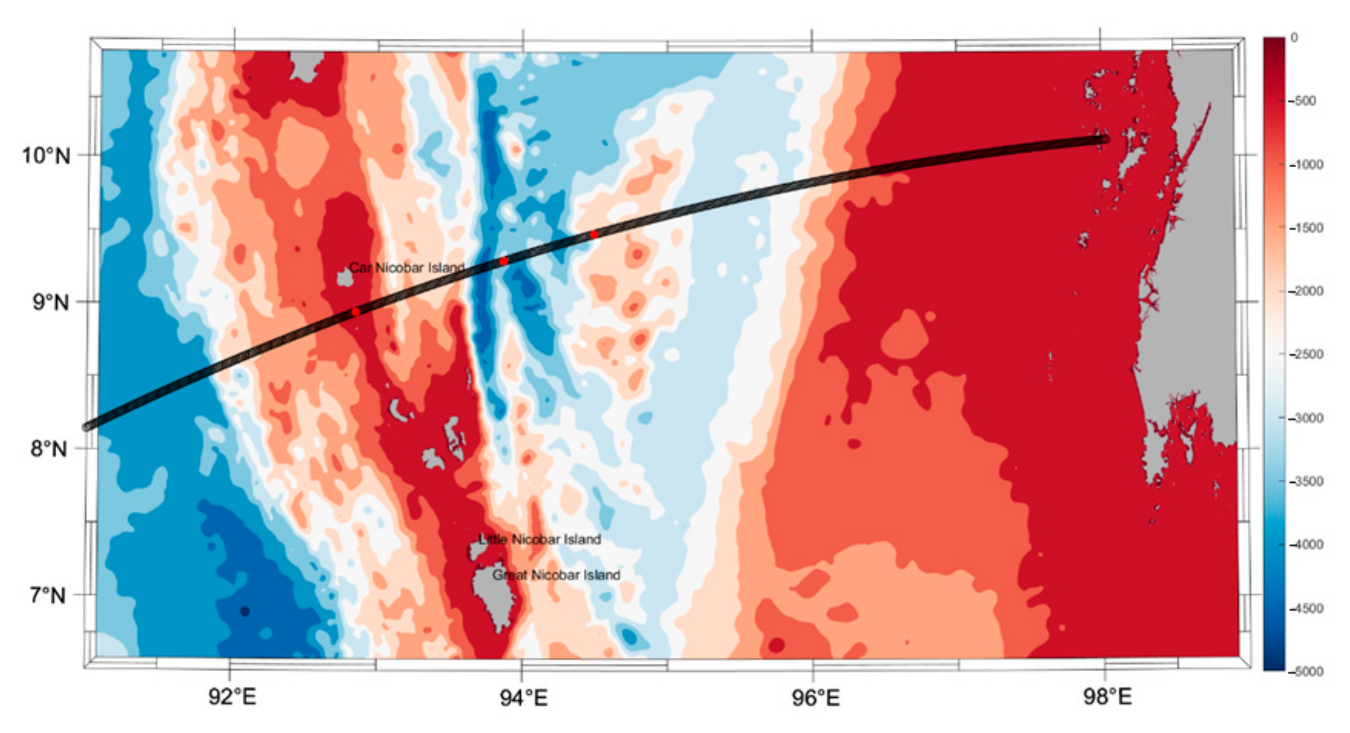
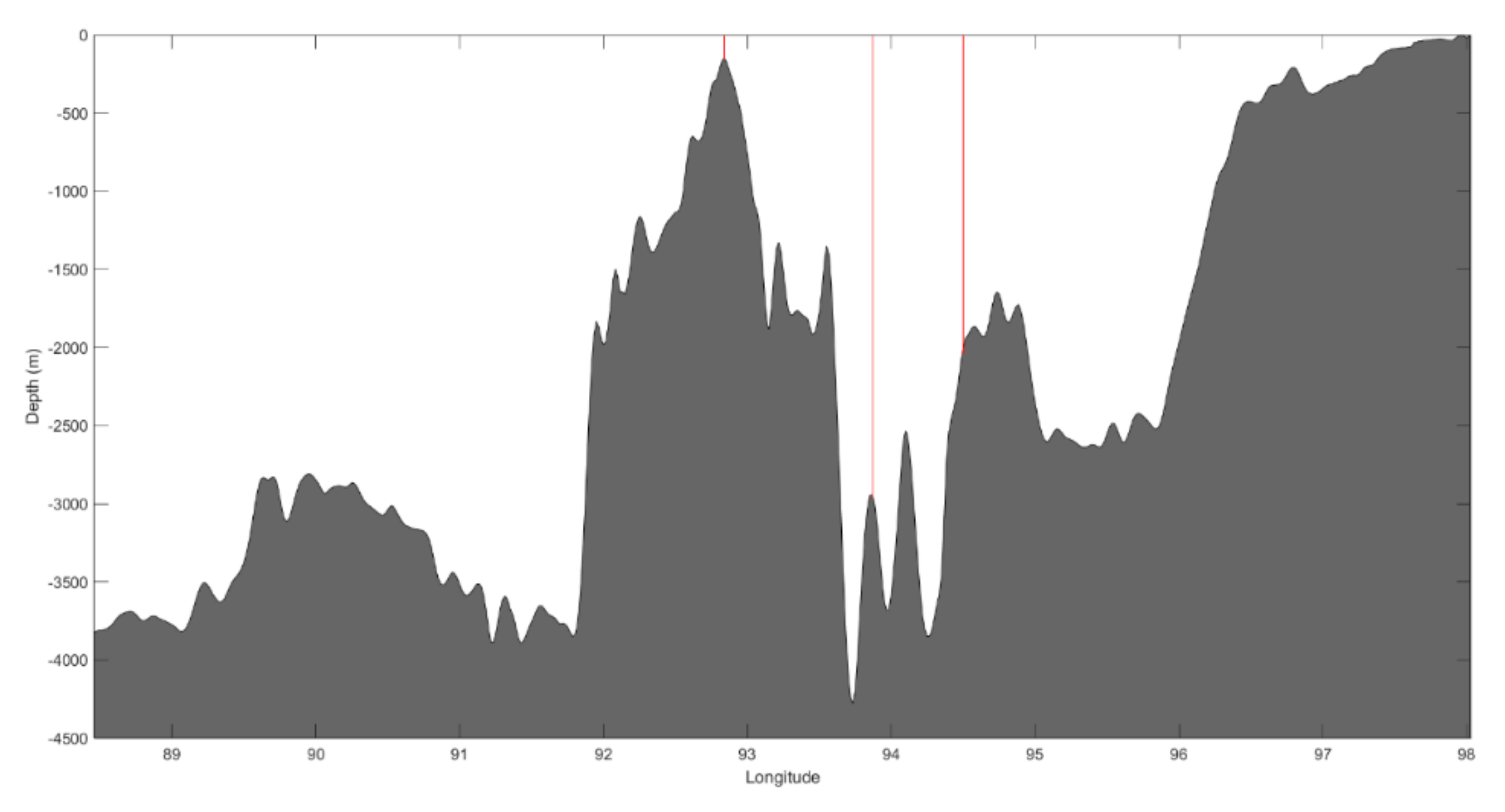
Figure 1 and
Figure 2 show the bathymetry of the central Andaman Sea and the cross-section used for model simulations. The cross-section was chosen based on the fact that it passes over the generation location and follows the direction of propagation of the Mode-1 ISWs. Two output locations, that represent potential study sites are arbitrarily chosen to the east of the generation location. Three locations are identified in
Figure 1 and
Figure 2: The westernmost location is the generation site where mode-1 waves are produced; the two locations to the east are locations where model outputs were analysed in detail and metocean criteria was produced. The distance between the generation and the first output locations is approximately 100 km which corresponds to nearly the distance between leading wave of the crests. Note that ISW propagate in packets of 2 to 10 waves with wavelengths of 5 to 10 km. The packet length is typically 15 to 50 km. The leading wave in a packet is typically the one with largest amplitude. The second output location is 40 km to the east of the first one.
As no in-situ data are available for validation purposes, the model was compared to other datasets, mostly taken from satellites, for the Central Andaman Sea, including phase speed, interpacket distances and other relevant characteristics.
In order to estimate the phase speed for long-lived mode-1 waves time series of currents have been extracted for the 2 locations shown in
Figure 1 and
Figure 2. The leading waves have been detected by using an algorithm to calculate local maximum acceleration with a threshold of 0.01 m/s
2 at 100 m depth which has been identified as the level where consistently higher currents are obtained. The time difference between the occurrence of maximum at the two output locations was then used to compute the phase speed since the distance is known. The technique also allows the counting of internal solitary wave events and therefore the establishment of the frequency of their occurrence.
The estimated frequency of events has been monthly averaged over the 10 years.
Table 1 summarizes the results derived from the model for phase speed, frequency of events and mixed layer depth at the western output location. In addition, presented are the mixed layer depths extracted for the area from the World Ocean Atlas, Monterey and Levitus [
59]. The selected mixed layer depth from World Ocean Atlas is using the temperature criteria: a temperature change from the ocean surface of 0.5 °C. The same criteria were adopted to evaluate the mixed layer depth from the model results.
Other relevant statistics can be derived once the events are isolated and selected. In particular, it is possible to characterize the current speeds associated to ISWs.
Table 2 shows the statistics for the maximum speeds associated to each event at the western output location. The statistics for maximum speed were built by selecting the largest current speed in each individual event at 125 m depth where, typically current is at maximum. Note that maximum speeds are found in November, December and January while minimum are found in July and August with a clear correspondence to the seasonal evolution of the mixed layer depth.
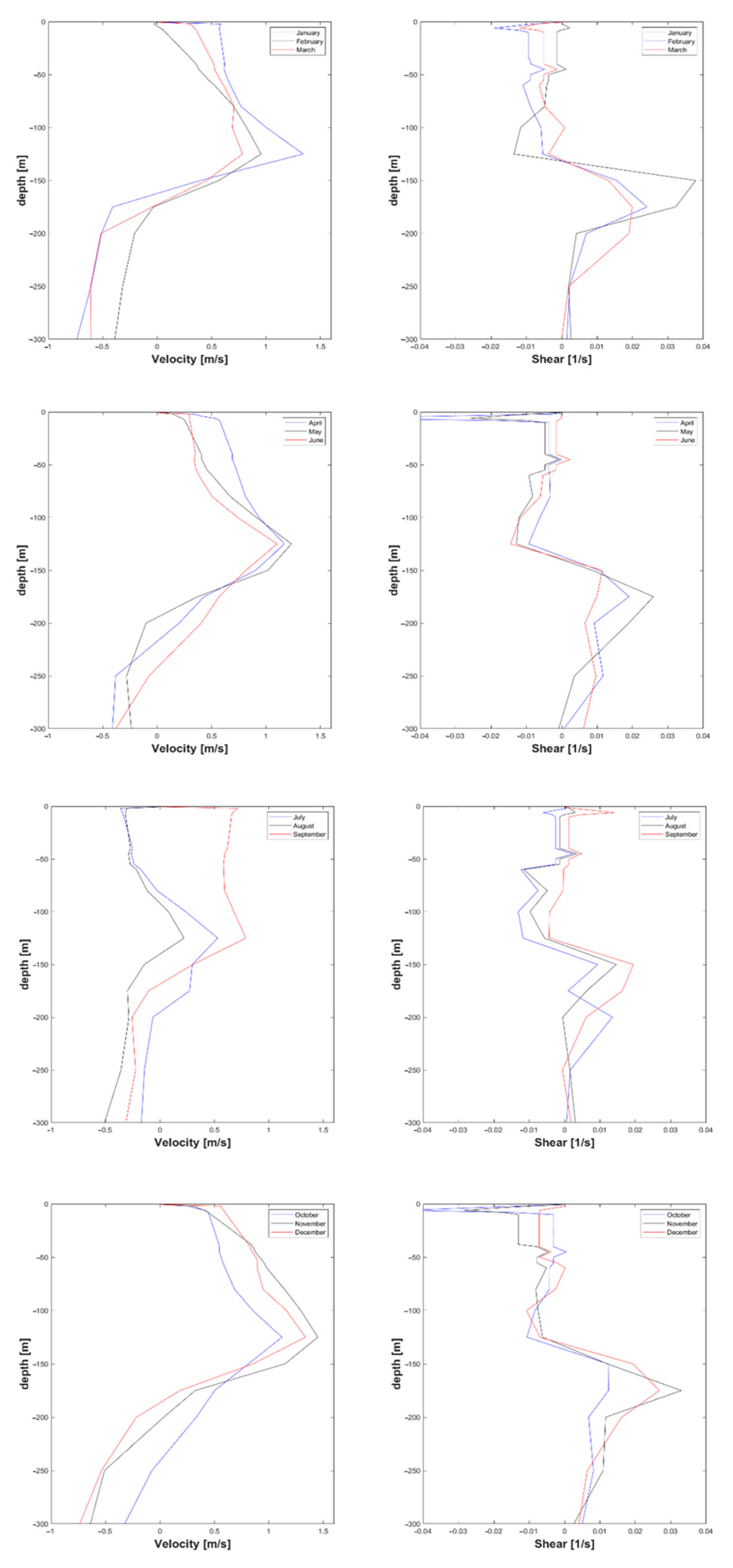
With the identification of maximum events per month over the 10 years of simulation it is also possible to compute the associated vertical profiles and shear which quite important to quantify vertical variation of velocity during extremes.
Figure 3 shows the vertical profile corresponding to the maximum velocity observed each month over the 10-year simulation. The structure shown is typical for mode-1 waves with a maximum speed at the base of the mixed layer and the correspondent maximum shear below the maximum velocity. Typical maximum shear values are in the range 0.02 to 0.04 L/s.
Extreme criteria at the western output location for specific return periods were obtained by carrying an extreme value analysis over the 10-year dataset at the depth of 125 m where maximum velocity is commonly observed. The derivation of extremes was done by using the peaks over threshold method. The threshold is obviously arbitrary, and it was adjusted to better fit the data available. The threshold chosen was 0.8 m/s. Three distributions were fitted to the time series of event maxima: Weibull, Generalised Pareto and Fisher-Tippet 1. The adjustment used the method of maximum likelihood and the method of moments. The best fit was obtained by using the Generalised Pareto distribution adjusted by the maximum likelihood method and the extreme criteria obtained is shown in
Table 3.
4. Discussion
The major goal of this work was to derive reliable statistics from long-term time series of currents obtained from numerical models. The Central Andaman Sea was chosen to test the methodology. A 2D-V non-hydrostatic model was used to simulate the generation of ISW south of Car Nicobar Island and their propagation eastward into the Andaman Sea. The generation location was chosen based on findings from several authors namely, Raju et al. [
55] and Sun et al. [
54] who produced comprehensive studies based on satellite imagery.
In the absence of in-situ data for model validation, other strategies were used to infer on the quality of the results. The phase speeds for long-lived mode-1 waves were computed with an algorithm to detect the leading wave on a ISWs packet based on accelerations. The monthly averaged phase speeds calculated for the area of the Central Andaman Sea comprised between 94° and 94.5° E (with water depths ranging from 2000 to 3500 m) are within the range of observations. Model results provide values between 2.33 and 2.50 m/s in line with observations and theoretical calculations presented by Tensubam et al. [
52]. However, this study does not corroborate the finding from Tensubam et al. [
52] regarding the seasonality of phase speeds. In their paper, Tensubam et al. [
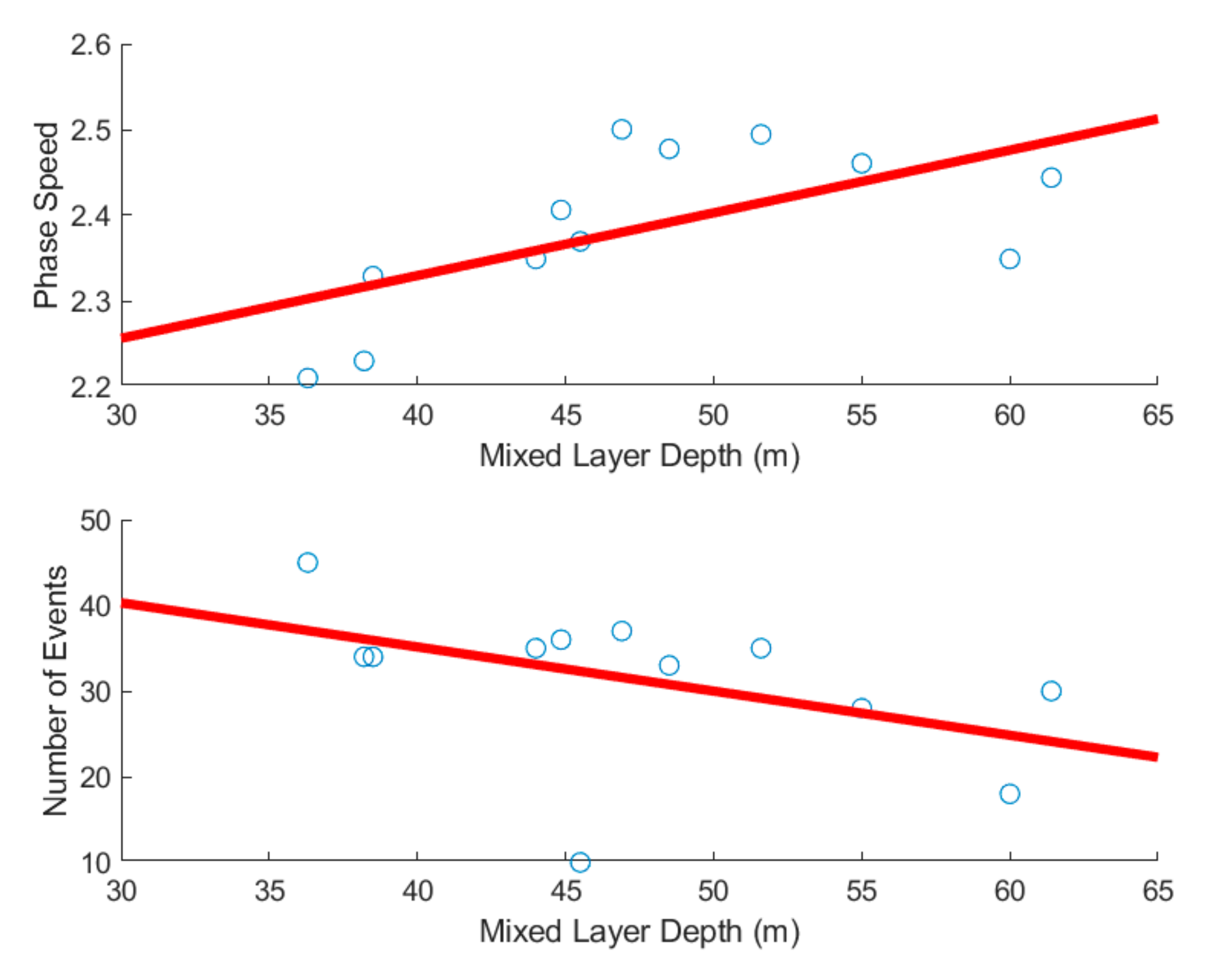
52] reported higher phase speeds in January/December in the SE Andaman Sea. They attribute this seasonal variability to changes in stratification and mixed layer depth. The model results show an increase in phase speed with increasing mixed layer depth with a correlation 0.62. In addition, the number of events seems correlated with the mixed layer depth. A negative correlation of -0.51 was obtained indicating that occurrence of ISWs is more likely during high-stratification periods.
Figure 4 shows the dependence between phase speed, frequency of events and the mixed layer depth.
The time that it takes for a wave packet to hit a specific location can be derived either from the computed phase speed if it is assumed that there are no relevant gradients or by identifying the moment of generation and the moment when the leading wave of a packet is detected over a specific location. Using the first method and given that (i) according to Tensubam et al. [
52] and theoretical approach the phase speed doesn’t change too much for water depths larger than 1000 m, (ii) the distance between source and the target location described in
Section 3 is 100 km, the average time that it takes for the leading wave to hit the site is 11 h and 39 min. The interpacket distance computed using the same premises and the fact that the associated period is 12 h and 25 min is around 106 km well within other estimates such as Sun et al. [
54] and Tensubam et al. [
52]. To use the second method, the generation mechanism needs to be understood. Given the complexity of the generation process it is not always easy to identify the mechanism responsible for the generation. Magalhaes and da Silva [
56] examined the characteristics of the ISWs propagating in the Central Andaman Sea with origin in 2 different areas: (i) south of Car Nicobar Island—the same location considered in this paper, and (ii) to the North, along 10° N with origin over in the Ten Degree Channel. For the first case, typical long-lived mode-1 waves were identified with an interpacket distance of about 100 km. Short scale mode-1wave tails were also identified. For waves generated in the Ten Degree Channel no long-lived mode-1 waves were identified. The paper from Magalhaes and da Silva [
56] then discusses the mechanism of generation of the mode-2 waves that are generated in the Ten Degree Channel. For long-lived mode-1 waves produced south of the Car Nicobar Island, Maxworthy [
60] is probably the one that best fits the observations. The mechanism can be roughly described as follows: when ebb tidal currents flow westward over the shallow sill they generate a lee-wave depression to the west side of the sill. When the tidal currents reverse to weak flood tidal current flowing eastward, the lee-wave escapes over the sill and evolves into the ISW propagating to the east across the Andaman Sea. Therefore, the time to travel between the source and the target location can be computed as the being the time between slack over the generation site and the instant when the leading wave is detected at the output location 100 km to the east. Using this method, the computed time for the leading wave in a packet to travel from source to destination is 11 h and 32 min in close agreement with the previous estimation.
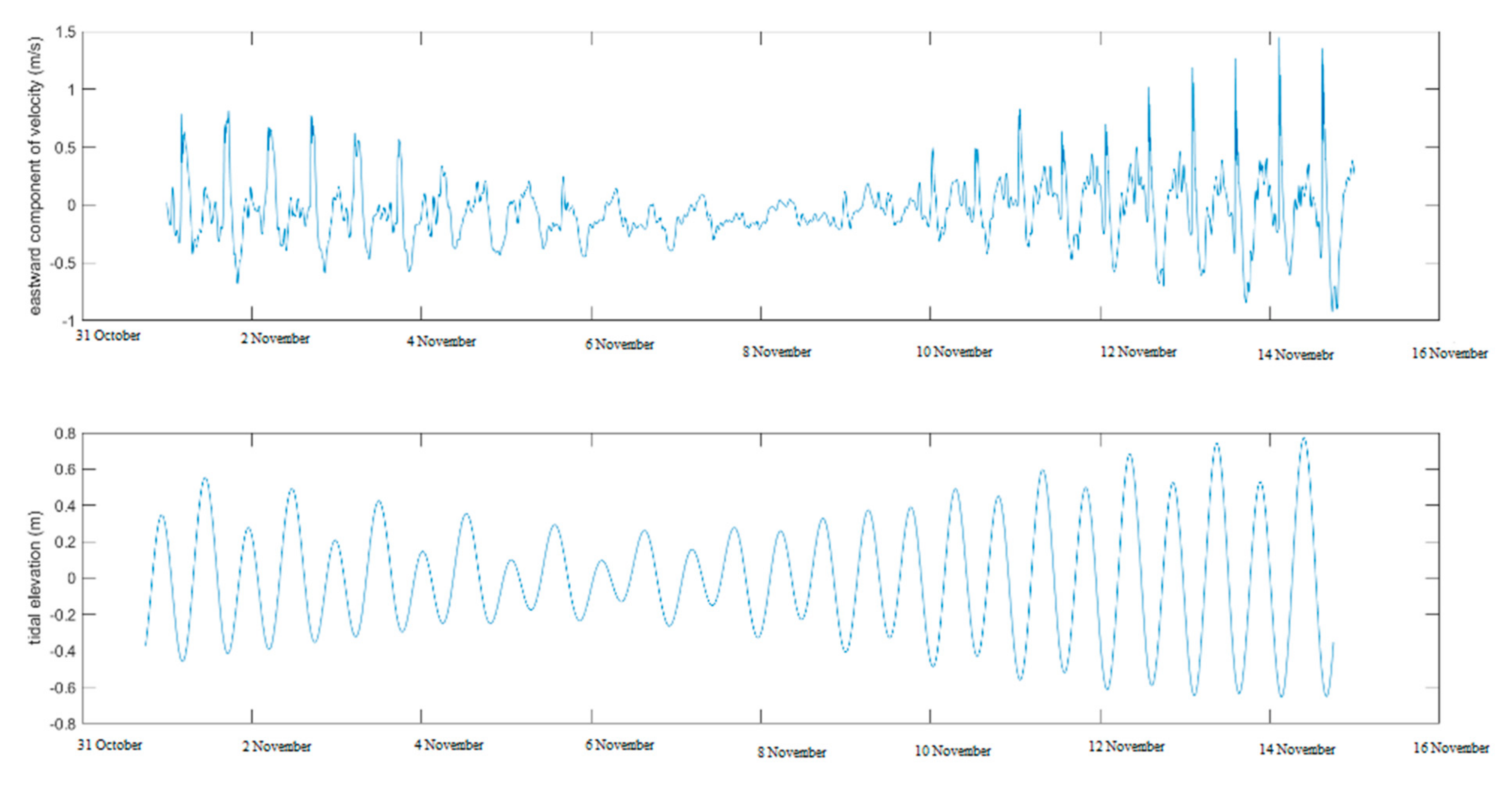
To evaluate the relation between the tidal cycle and the amplitude of the current associated to ISWs it is useful to plot the tidal water levels at the generation location and currents at the target.
Figure 5 shows the water levels at the generation location and the eastward current at 125 m depth over the output location 100 km to the east. It is clear the relation between the spring-neap tidal cycle with stronger currents being obtained during the spring stage. Actually, during the period with lowest tidal amplitudes shown in the figure (from 6 to 10 November) there are no events while later, from 10 November onwards, the eastward component of water current reaches values up to 1.5 m/s.
The results discussed so far contain valuable information for programming operations and for design regarding offshore industry. The model results proved to be reliable from the physical point of view and when compared to parameters such as phase speed and interpacket distance. To fully prove the validity of the model, available measurements of current speed and thermocline displacement are required. However, as a proof of concept these model results obtained for a long-term hindcast were used to derive metocean criteria by means of extreme value analysis. The currents associated to return periods of 1, 10, 50, 100 and 1000 years were derived by adjusting different distributions with different methods. The best estimate was obtained with the Generalised Pareto distribution adjusted by the maximum likelihood method. The results obtained are satisfactory when compared to the data although they seem to be a conservative estimate. It would be interesting in the future to compare model and in situ data in order to establish criteria at least to the lower return periods.
5. Conclusions
Following the methodology presented by Ali et al. [
37] a 2D-V model was implemented in the Central Andaman Sea in order to simulate the propagation of ISW and derive relevant parameters for design and operations for the offshore industry. The model used realistic topography along the cross-section considered, and realistic boundary and initial conditions (tidal components, temperature and salinity). The model output was analyzed at two different locations arbitrarily chosen. To achieve the proposed goal the model ran for 10 years continuously. With the resolution used, the model took 10 wall clock hours to simulate a month using 36 2.9 GHz Intel Xeon E5-2666 v3 processors or 50 days to run the whole hindcast. To our knowledge this was the first time that such and hindcast was produced for the purpose of deriving operational and design criteria.
The model was compared with available literature of the area, namely mixed layer depth, phase speed and related parameters such as interpacket distance. The results are in close agreement with the available data. In particular, the model has reproduced quite well the seasonal variability of the mixed layer depth and the phase speed. The frequency of events also shows a relevant correlation with mixed layer depth and stratification.
The phase speeds computed are in the range 2.21 m/s in March when the mixed layer depth is at the minimum (36.3 m) and 2.5 m/s in November that corresponds to the second highest value for the mixed layer depth (58 m). The average time that it takes for a wave to travel from generation location to a point 100 km to the east is about 11 h and 30 min, implying an interpacket distance of 106 km. The computation of such a time using two different methods shows that for depths larger than a certain threshold the phase speed is nearly independent of water depth.
The frequency of events is at maximum in March when the mixed layer depth in minimum. Physically this means that when the stratification is stronger the Baines [
58] potential for generation is amplified and therefore the number of events is increased. Conversely, when the mixed layer depth is at maximum, the stratification is weaker and the number of events is lower. This is the case for June, July and August.
Monthly averaged maximum speeds were calculated based on event selection by using an acceleration threshold at 100 m depth. Most importantly the maximum speeds for every month were computed. There are significant differences between July to September and November to January. The lowest maximum speed was obtained for August (0.22 m/s) while the highest value is 1.49 m/s in November.
Finally, extreme value analysis was conducted on the time series of events by using the peaks over threshold method. The obtained series of peaks was fitted by using the maximum likelihood method to adjust a Generalised Pareto distribution. The currents associated to the return periods of 1, 10, 50, 100 and 1000 years range from 1.67 m/s to 1.84 m/s.
The methodology presented to produce long-time series of currents related to the passage of ISWs signifies a valid tool to produce robust information for design and operations for offshore industry. In particular, the proposed methodology can be used in lieu of expensive metocean observation campaigns with limited time coverage. However, in order to have a reliable dataset a set of measurements is always required for validation purposes. The methodology proposed allows the derivation of extreme criteria. The present model has been validated for a limited number of parameters that does not include currents and thermocline displacements. Additional work is compulsory, including a full validation of the collected datasets that may be affected by ISWs associated with the offshore industry.


