Abstract
Three-dimensional numerical simulations were performed for different flow rates and various geometrical parameters of step-pools in steep open channels to gain insight into the occurrence of energy loss and its dependence on the flow structure. For a given channel with step-pools, energy loss varied only marginally with increasing flow rate in the nappe and transition flow regimes, while it increased in the skimming regime. Energy loss is positively correlated with the size of the recirculation zone, velocity in the recirculation zone and the vorticity. For the same flow rate, energy loss increased by 31.6% when the horizontal face inclination increased from 2° to 10°, while it decreased by 58.6% when the vertical face inclination increased from 40° to 70°. In a channel with several step-pools, cumulative energy loss is linearly related to the number of step-pools, for nappe and transition flows. However, it is a nonlinear function for skimming flows.
1. Introduction
Analysis of flow regimes in mountainous streams is important as the flow may carry large amounts of sediment, which affects the live storage of downstream reservoirs and the stream morphology [1,2]. It is important from the perspective of stream ecology, especially in wet and dry tropics, where these streams and their surroundings are hotspots of bio-diversity [3,4,5]. It is also important for developing steady and unsteady mathematical models [6], which can be used for the planning and design of river restoration and other hydraulic structures.
Mountainous streams are characterized by step-pools. Many studies have been carried out in the past on natural step-pool streams using field data to understand: Changes in characteristics of a step-pool system as a function of flow rate [2,7]; standardizing geomorphic definitions of step height, step wavelength, active width, drainage area, slope and particle size [8]; entropy of step-pools, bed slope and bed friction [9]; the effect of sediment supply on the stability of step-pools [10] and step-pool structure [11]; design of scour depth and pool depth [12]; the effect of step-pools on ecology and flow resistance [13]. Recently, Kalathil and Chandra [14] provided an extensive review of work carried out on step-pool hydrodynamics in mountainous streams.
An experimental study was conducted to understand bed level changes in step-pools due to hydraulic properties [15]. Peterson and Mohanty [16] and Sindelar and Smart [17] conducted laboratory experiments to understand the occurrence of different flow regimes and their effect on step-pool stability. In the nappe flow regime, flow alternates between subcritical and supercritical conditions with the critical flow over each step [17]. The flow is supercritical and skims over the tops of the steps having almost flat water surface in the skimming regime [17,18]. The transition flow regime is characterized by the presence of standing waves and oscillating jets of flow. Among the three flow regimes detected, transition flow regime had the most critical effect on stability [17]. Though some studies have identified the flow regimes in step channels, understanding of the energy loss variation in the three flow regimes requires systematic investigation. Several studies have attempted to investigate energy loss in step-pools and spillways with step-pools (a brief discussion is in the following section), as step-pools are the major energy dissipaters in step channel.
Understanding energy loss in step-pools is one of the primary steps towards the development of flow models for mountainous channels as well as for designing stepped spillways [19,20]. In a mountainous stream, the energy loss due to dissipation of turbulent energy in the pools is more significant than grain or form drag [21,22]. Lee and Ferguson [23] found that flow resistance changed rapidly as discharge increased and did not conform to simple log law behavior. Chin [2] found that around 90% of potential energy dissipation was observed for low flow rates in step-pools and effective energy dissipation is greater at low flows. Based on field data from Rio Cordon, Italy, Comiti et al. [7,24] attempted to obtain a relationship between dimensionless velocity, , and dimensionless unit flow rate, , and step geometry, h/l, and channel gradient or slope, S, in which = flow velocity; = bed roughness; = step height; = step length; = acceleration due to gravity; q = unit discharge. However, this relationship is valid for a small range of unit discharge (0.02–0.4 m2 s−1), but not applicable to high flow conditions. A thorough investigation of energy loss induced by spillway with flat steps [25,26], flat steps with end sills (pooled steps) [25] and a combination of the two cases was carried out [25,26]. In the above studies, the pooling effect of water was created using end sills but not with the inclination of step. Agostino and Michelini [27] provided a predictive equation for relative energy loss at a step as a function of the ratio between pool depth and step height, for values of the ratio less than around 0.80. Andre [28], Nikseresht et al. [29], Peyras et al. [30], Chinnarasri and Wongwises [19] investigated flow structure within stepped chutes, spillway with step-pools, stepped gabions, stepped chutes, respectively. Most of these studies, which were essentially conducted for stepped spillways, did not consider the formation of water pooling due to vertical and horizontal face inclinations which is common in natural step-pool systems. Very few studies [19,29] considered the effect of horizontal face inclination. In the studies conducted by Nikseresht et al. [29] and Chinnarasri and Wongwises [19], the slope of stepped spillways varied from 35° to 50° and from 30° to 60°, respectively. However, the slope of step-pools mostly varies from 2.9° to 11.4° in nature [27]. Moreover, the inclination of horizontal face was varied from 10° to 30° in the study by Chinnarasri and Wongwises [19], while in nature; the horizontal inclination for step-pools in mountain streams usually varies between 2° and 10°. Moreover, energy loss variation under the sequence of flow regimes through low flows to high flows for step-pools is missing in their studies.
Over the last few years, myriad research, e.g., [31,32,33,34,35] has proved that three-dimensional (3D) computational fluid dynamics (CFD) models could be a practical and robust tool to investigate flow structure in complex flow fields. With regard to step-pools, Chen et al. [36] used volume of fluid (VOF) technique with turbulence model to simulate flow structure on stepped spillways. Nikseresht et al. [29] used ANSYS-FLUENT model for analyzing flow in step-pool spillways. Effect of slope on energy dissipation was investigated by Heidari and Ghassemi [37] using CFD model for stepped spillways. Chiu et al. [38] evaluated the FLOW-3D model performance using experimental results for a vertical drop. Bombardelli et al. [39] compared measured time-averaged velocities for the flows in stepped spillway using k ε, RNG k ε turbulent models and found that the results did not significantly vary between the turbulent models. Morovati and Eghbalzadeh [40], Bayon et al. [41] and Valero et al. [42] used RNG k ε model and it was found to be better than other models. Abdulla [43] evaluated the performance of different turbulent models (k ε, RNG k ε and SST) using ANSYS-CFX for Froude number varying from 1.2 to 2.0 for flows around bridge piers where flow separation was significant. insignificant difference was found between the turbulent models with least computational time and cost for k ε model.
Building on insights from previous investigations, this study used a CFD model to investigate the occurrence of energy loss due to different flow rates and various geometrical parameters of step-pools in a steep channel. Following questions are explored in this particular study: (i) For a given step-pool geometry, how does the energy loss vary with flow rate in a sequence of flow regimes; (ii) how does the flow structure change as the flow rate increases and thus affect the energy loss; (iii) how is the energy loss influenced by the vertical and horizontal face inclinations of the pool; and (iv) what is the interaction effect between step-pools in a sequence of step-pools and how does the energy loss vary with distance? Numerical results presented in this study are expected to provide a better understanding of flow structure and energy loss in steep open channels with step-pools, and help in the development of a simple but reasonably accurate empirical equation for energy loss in step-pool channels, in the context of hydrodynamic models for mountainous channels.
2. Methodology
2.1. Description of CFD Model
In recent years, CFD models have been used to understand flow structure in complex open channel flows including stepped spillways, e.g., [31,32,36,38,44]. Following a similar methodology, the research issues listed earlier are addressed in this paper by (i) first evaluating the performance of ANSYS-CFX model to reproduce flow characteristics in a stepped spillway and in step-pools using data available in the literature, (ii) then utilizing the validated software to conduct numerical simulations for flow in nature-like step-pools and (iii) finally analyzing the effects of flow rate and step-pool geometry on flow structure and energy losses.
In the present work, commercially available CFD model ANSYS-CFX [45] was selected for the study. The software solves the three-dimensional Reynolds-Averaged Navier–Stokes (RANS) equations along with the standard turbulence model [46], using a finite-volume method. ANSYS-CFX uses a multiphase model, with air and water representing the two phases of fluid, to model the “free-surface” sing the Volume of Fluid (VOF) method [47]. VOF solves a single set of momentum equations throughout the domain, while keeping track of the volume of phases in each computational cell. The software program solves the continuity and momentum equations in tensor form as follows [45]:
Continuity equation:
Momentum equation:
where, is the fluid density; is the water density; is the air density; is the water volume fraction; is the air volume fraction; is fluid velocity; is the pressure; is the gravitational force; is the turbulent kinetic energy; is the Kronecker delta; is the molecular viscosity of the fluid; is the molecular viscosity of water; is the molecular viscosity of air; and is the turbulent viscosity of the fluid. The transport equation for and are as below, respectively:
The standard turbulence model was chosen based on the performances of previous model studies from the literature, e.g., [31,32,35,36,39,43] as discussed in the introduction. The governing equations for turbulence model are as follows [45]:
where, is 1; is 1.30; is 1.45; is 1.90; is 0.09; is 1; is the turbulent kinetic energy; is the energy dissipation rate; is turbulence production due to viscous forces; represent the influence of the buoyancy forces. A curvature correction factor is used to consider streamline curvature. The detailed information on is given by Spalart and Shur [44]. In the present study, high-resolution scheme was used, where central differencing second order advection scheme and upwind difference scheme are combined. The combined scheme provides sufficiently accurate solutions to capture complex flow conditions whereas the upwind difference advection scheme is not good enough since it uses first-order advection scheme [45]. In all numerical simulations, mesh characteristic (Y+) was maintained less than 300 and more than 30 to satisfy dimensionless wall height criteria. The details of boundary conditions, convergence criteria and time step are discussed in Section 2.2 to illustrate along with Test Cases used in this study.
2.2. Testing and Validation of ANSYS-CFX
Three datasets from earlier studies [17,19,36] were used to test and validate the ANSYS-CFX. Chen et al. [36] conducted experiments on a stepped-spillway with varying step size and obtained pressure variation data using piezometers tubes. Chinnarasri and Wongwises [19] conducted experiments on a stepped spillway with uniform size. Energy loss due to steps was measured for different experimental scenarios when flow rate was varied from 0.004 m3 s−1 to 0.068 m3 s−1. The experimental setups used in these two studies are shown schematically in Figure 1a,b, respectively. Sindelar and Smart [17] conducted experiments on a step-pool system, as shown schematically in Figure 1c. Gravel with diameter of 8 mm to 16 mm was glued to acrylic bottom of the flume. Sixty-nine wooden blocks and one aluminum block were used to create nine step-pool units. The blocks had a base area of 0.1 m × 0.1 m and an effective height of 0.08 m. All blocks were placed with a gap of 0.622 m and 0.008 m in longitudinal and transverse directions of the flume, respectively. A total of 14 pressure transducers were installed within the aluminum block. It was located at midpoint for sixth step-pool unit. Total pressure head profiles were measured for transition flow regime and occurrence of different flow regimes was studied. Dimensions of the flumes, steps and other data for all the three experiments are summarized in Table 1.
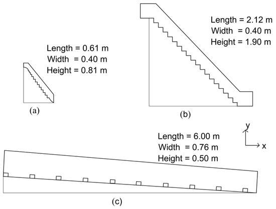
Figure 1.
Schematic of test cases for assessment of ANSYS-CFX package: (a) Stepped spillway with varying step sizes; (b) stepped spillway with uniform step sizes; (c) step-pools created by a group of cuboid shaped roughness elements.

Table 1.
Experimental data used for model validation.
To use the data in Table 1 for simulations with ANSYS-CFX a number of boundary conditions were defined. Details of boundary conditions in all numerical simulations in the present study are as follows. Flow rate with 5% turbulent intensity was specified at the inlet or left boundary of the flow domain. The pressure was specified at the outlet or right boundary, by assuming that the pressure was hydrostatically distributed, for the specified flow depth. Atmospheric pressure condition was specified at the top of the flow domain. Bottom of flow domain was treated as smooth boundary for Test Cases 1 [36] and 2 [19]. For the Test Case 3 [17], bottom boundary was treated as a rough boundary with a value of 2.55 × 10⁻⁴ m for equivalent sand grain roughness height corresponding to rounded gravel. For all wooden blocks and aluminum block, roughness value was given as 0.0008 m and no-slip boundary condition was applied to bottom and blocks. Symmetry sidewall conditions were specified for Test Cases 1 and 2 and smooth walls with no-slip conditions were specified for the Test Case 3.
The convergence criterion in all simulations (steady state flow conditions) was 0.0001 and convergence was achieved within 2000 iterations with a physical time scale of 0.4 s. Unstructured tetrahedral computational mesh was created using the “ICEM CFD” subroutine available in the ANSYS-CFX. Mesh close to the bottom boundary was refined using inflation technique with transition ratio 0.77, 12 maximum number of layers, 1.2 growth rate to make sure the first mesh was within logarithmic region as shown in supplementary Figure S1b. Experimental observations provided by Sindelar and Smart [17] were used to test for grid convergence. Four different mesh sizes with a maximum mesh size of 0.02 m, 0.015 m, 0.01 m and 0.0075 m were used for grid sensitive analysis. Measured pressure variation at the downstream face of aluminum block is used for benchmarking as shown in Figure 2. The total number of nodes and elements varied from 859595 to 2472351 and from 3361613 to 8125059. A blend factor of ~1 is used in high resolution numerical scheme which may create oscillation in the results especially when geometry is symmetrical and mesh is not symmetrical. However, the results produced using the high resolution numerical scheme are more accurate than those obtained using other scheme (upwind difference advection scheme) available in ANSYS CFX [45]. The coarse mesh is found to be more symmetrical than fine mesh in this study. Therefore, minor oscillations are found in Figure 2 for fine mesh. The numerically simulated pressure profile with a maximum mesh size of 0.01 m is satisfactory. It can be observed from Figure 2 that the difference in results with 0.0075 and 0.01 m mesh sizes is insignificant.
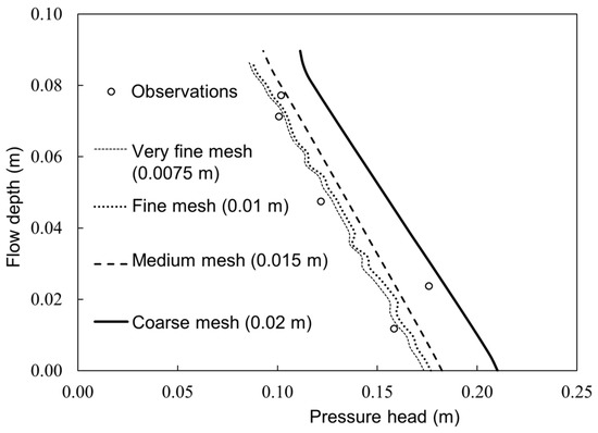
Figure 2.
Mesh sensitivity analysis: Simulated pressure profile at downstream face of block.
The performance of the model was determined using three goodness-of-fit indices:
where and are observed data and simulated results, respectively. indicates the average of all the observed values and is the number of data points.
Numerically simulated horizontal and vertical pressure profiles are compared with experimental data for Test Case 1 as shown in Figure 3a,f. Pressure profiles were collected on horizontal and vertical surfaces for fifth, ninth and 13th steps. Performance indices for the simulations for all three test cases are presented in Table 2.
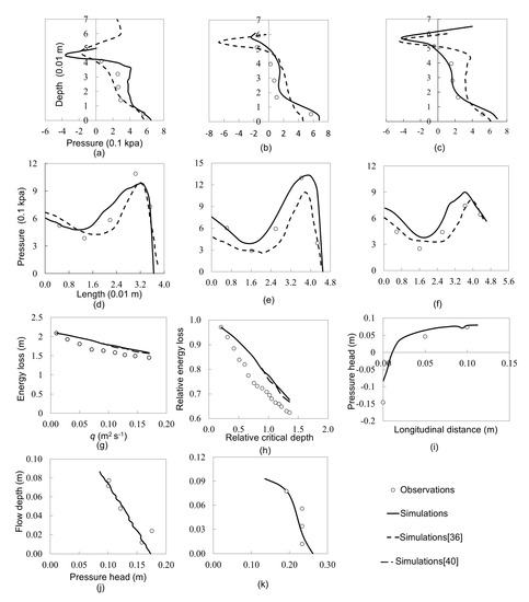
Figure 3.
Observed and simulated pressure profiles for Test Case 1: (a) Vertical step number—5; (b) vertical step number—9; (c) vertical step number—13; (d) horizontal step number—5; (e) horizontal step number—9; (f) horizontal step number—13; relative energy loss in Test Case 2: (g) Variation with flow rate; (h) variation with critical flow depth; pressure variation in Test Case 3: (i) Top face; (j) downstream face and (k) upstream face.
Table 2.
Performance indices for validation tests.
It can be observed that the correlation (Test Case 1: 0.65 to 0.93; Test Case 2: 0.52 to 0.56; Test Case 3: 0.85 to 0.96) between observed and modeled profiles is satisfactory. Numerically simulated profiles by Chen et al. [36] are also compared with experimental data in Figure 3a,f. It was observed that all three performance indices were marginally better for present simulations (RMSE: 0.56 to 1.03 Kpa; Bias: 0.76 to 1.01 Kpa; E: 0.65 to 0.93) as compared to the simulations reported by Chen et al. [36] (RMSE: 0.61 to 1.60 Kpa; Bias: −0.88 to −1.26 Kpa; E: 0.65 to 0.85). Simulated energy loss in Test Case 2 was compared with experimental data [19] in Figure 3g. It can be observed from Figure 3g that the energy loss decreased as the flow rate increased. Moreover, the relative energy loss (ratio between energy loss due to steps and total energy at the crest of first step) decreased as the relative critical flow depth (ratio between critical depth and step height) increased (Figure 3h). Nikseresht et al. [29] had performed numerical simulations for this case earlier. Their results are also presented in Figure 3g,h. It can be observed that the difference in results obtained in the present study and results reported by Nikseresht et al. [29] is insignificant. In Test Case 3, total pressure head profiles at upstream, downstream and top face of aluminum test block in the experiments conducted by Sindelar and Smart [17] were compared with the simulated results. The results are presented in Figure 3i,k. It can be observed in Figure 3i–k and Table 2 that the numerically simulated results matched satisfactorily with the observed values in the experiment (RMSE: 0.012 to 0.037 m; Bias: −0.028 to 0.006 m; E: 0.85 to 0.96).
It can be concluded from the results presented in this section and from previous studies [31,32,33,35,48,49] that the ANSYS-CFX model can be effectively used for performing numerical experiments to simulate flows in step-pools in steep channels. Results obtained from such numerical experiments can be analyzed to gain insight into the energy loss due to step-pools in mountainous channels.
2.3. Numerical Experiments for Energy Loss
The validated ANSYS-CFX model was utilized to conduct numerical experimental runs for energy loss in nature-like step-pools in steep open channels. The photographs shown in Figure 4a–c show a natural step-pool, skimming flow and nappe flow in a mountainous channel in the Western Ghats, India. Based on the above photograph, and photographs of mountainous channels available in the literature, a sequence of nature-like-step such as shown in Figure 5 was assumed for numerical experimental runs. Unlike a stepped spillway, the nature-like step-pool has both vertical and horizontal inclinations at each step. All numerical experimental runs were conducted for different supercritical flows at the crest of the first step. Numerical experimental runs were conducted for different step-pool geometries and flow conditions as presented in Table 3 and Table 4. The total length (L), height (H) and width of the computational domain were 5.6 m, 0.5 m and 0.76 m, respectively. The length of the computational domain for upstream and downstream section from the inlet is 1.72 m and 4.03 m, respectively.
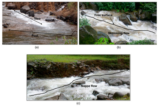
Figure 4.
Field photos: (a) Typical step-pool system (b) skimming flow (c) nappe flow.
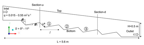
Figure 5.
Characteristic dimensions of step-pool system.
Table 3.
Details of numerical experiments for studying the effect of flow rate.
Table 4.
Details of numerical experiments for studying the effect of horizontal and vertical face inclinations on energy loss.
Flow varies in step-pool sequences in a mountainous channel, either during a flood or from season to season. This variation in flow affects the flow regime. Three distinct flow regimes: Nappe, transition and skimming flow have been observed in nature as well as earlier laboratory experiments. Therefore, a total of 13 (runs #1 to #13) numerical experimental runs were conducted for different Froude numbers at upstream section by varying the flow rate (q) in order to study the occurrence of different flow regimes in step-pools. Flow rate per unit width was varied from 0.015 m2 s−1 to 0.55 m2 s−1 (Table 3). In these numerical experimental runs, length (l), height (h), horizontal face inclination (), vertical step inclination () and slope of step-pool sequence were kept constant as 0.77 m, 0.162 m, 10°, 40° and 7.7°, respectively. The present numerical experimental runs were also used to understand how the energy loss in a step-pool system is affected by the flow regime. These values were chosen based on the field data reported by Agostino and Michelini [27].
Eight more (runs #14 to #21) numerical experiments were conducted to study the effect of step-pool geometry on the energy loss, where the values of the horizontal face inclination () and the vertical face inclination () (Figure 5) varied from 2° to 10° and 40° to 70°, respectively (Table 4). Variations in horizontal and vertical face inclinations affect the bed slope of step-pool. Along with the variation in inclinations of vertical and horizontal slopes, bed slope was varied such that value was kept constant at 0.21 as shown in Table 4 because several previous studies indicated that the energy loss strongly depends upon . Here, h = vertical distance from the crest of step to bottom most point in pool and l = horizontal distance from crest to next crest. All energy loss values were determined for step-pool 2. Slope of step-pool varied from 7.7° to 11°. Sand grain roughness (ks) value for step-pool bottom was specified as 2.55 × 10⁻⁴ m.
All numerical experiments were conducted for 3D flow conditions using ANSYS-CFX with specified (i) flow rate at the inflow section, (ii) flow depth at the outflow section and (iii) bed roughness (equivalent sand grain roughness height, ks). Boundary conditions were specified as described earlier. The total energy TEu at a section upstream (section u) and total energy TEd at a section downstream (section d) of step-pools (Figure 5) were determined. Energy loss (ΔE) between these sections “u” and “d” due to the three step-pools was calculated as the difference between TEu and TEd.
2.4. Dimensionless Parameters for Energy Loss
Energy loss due to step-pools was analyzed using a functional relationship proposed by Chinnarasri and Wongwises [19], extended to include additional non-dimensional parameters such as horizontal and vertical face inclinations to understand the water pooling effect.
where = energy loss between section u and d as shown in Figure 5; = average velocity at upstream section; = average flow depth at upstream section; l = step-pool length; h = step-pool height; = horizontal face inclination; = vertical face inclination; = relative energy loss; = Fu = Froude number at the upstream section; and = ratio between step-pool height to length. In this study, effects of , and Fu on the energy loss are investigated. Effect of the ratio between step-pool height and length was not investigated, as this effect has already been studied by many researchers [30,50].
3. Results and Discussions
3.1. Effect of Flow Rate
Velocity vectors and vorticity contours on the central vertical plane of the domain for three different unit flow rates (0.015, 0.16 and 0.55 m2 s−1) are shown in Figure 6 and Figure 7, respectively. The vorticity is the microscopic measure of rotation of fluid [45]. It can be observed that when the inflow rate was 0.015 m2 s−1, circulation occurred in the upper regions of the pool and free surface was almost horizontal. Velocity and vorticity in circulation zone varied from 0 to 0.35 m s−1, and from 6 to 30 s−1, respectively, and the flow was subcritical. This type of flow pattern is classified as “nappe” flow regime. For more details, the circulation pattern for nappe flow is shown in Figure 8 for three different inflow rates: q = 0.015 m2 s−1; q = 0.03 m2 s−1 and q = 0.075 m2 s−1 (at the verge of transition). It can be observed from Figure 8 that nappe flow occurred below the circulation zone in each pool for inflow rates 0.015 m2 s−1 and 0.03 m2 s−1. The circulation zone is shifted to almost bottom of the pool when the inflow rate was 0.075 m2 s−1 and the onset of the “transition flow” regime occurred (Figure 8c). Similarly, when the inflow rate was increased to 0.16 m2 s−1, circulation zones were shifted from the top to lower part of the pool. Moreover, velocity and vorticity in circulation zone increased as compared to nappe regime (0 to 0.56 m2 s−1; 13 to 30 s−1) and free surface was observed to be wavy (Figure 6b). When the flow rate was 0.55 m2 s−1, velocity and vorticity in circulation zones increased further up to 1 m s−1 and 30 s−1, respectively, and the wavy free surface disappeared, resulting in a horizontal free surface. This flow regime is classified as “skimming” flow regime. Similar flow regimes were observed for step-pools in experiments conducted by Sindelar and Smart [17] and Baki et al. [32].
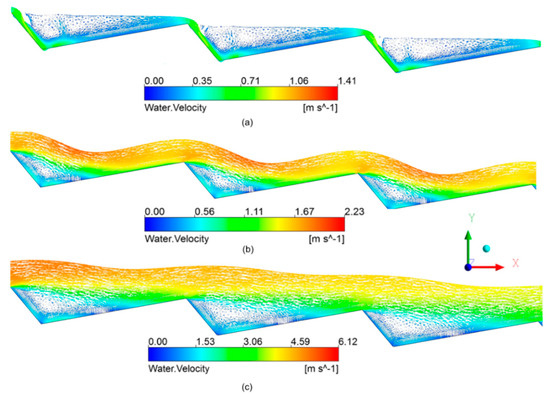
Figure 6.
Velocity vectors on central vertical plane for flow in step-pools: (a) Nappe flow (q = 0.015 m2 s−1); (b) transition flow (q = 0.16 m2 s−1); and (c) skimming flow (q = 0.55 m2 s−1).
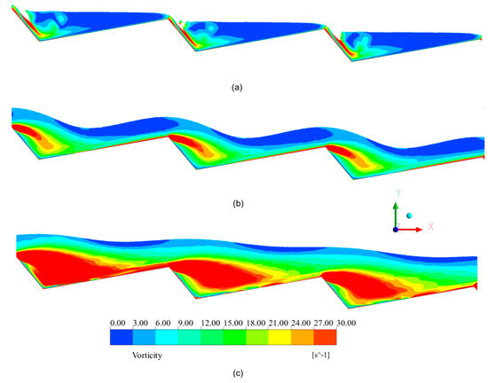
Figure 7.
Vorticity contours: (a) Nappe flow (q = 0.015 m2 s−1); (b) transition flow (q = 0.16 m2 s−1); and (c) skimming flow (q = 0.55 m2 s−1).
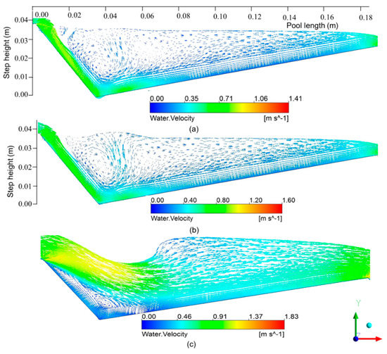
Figure 8.
Circulations in step-pool 2: (a) Nappe flow (q = 0.015 m2 s−1); (b) nappe flow (q = 0.03 m2 s−1); (c) nappe flow (q = 0.075 m2 s−1) on verge of transition flow.
Numerical results were used to estimate the energy loss in step-pool 2 and the results are presented in Figure 9. For nappe flow conditions, energy loss (ΔE) decreased marginally although the flow rate was increased by five times (Figure 9a). Darcy Weisbach friction factor (f) is calculated using the energy loss, average flow depth, velocity and length of step-pool 2. The variation of the friction factor with flow rate is shown in Figure 9a along with energy loss. It is noticed that f varied from 0.20 to 0.25 for nappe flow, 0.25 to 0.17 for transition flow and 0.17 to 0.15 for skimming flow. As expected, friction factor is high at low flow rate (0.015 m2 s−1 to 0.075 m2 s−1) and decreased at higher flow rates (0.075 m2 s−1 to 0.55 m2 s−1). However, energy loss increased from low flow rate (transition flow) to higher flow rate (skimming flow) and it is discussed below. It may be noted that for this range of variation in flow rate, Froude number at upstream section (Fu) remained almost constant at 1.50 (Figure 9b). Moreover, the length and height of the circulation zone were almost similar for all nappe flow simulations (Figure 8a,b). This resulted in only marginal variation in energy loss although the flow rate was increased by five times. It can be observed from Figure 8b that changing of flow regime from nappe flow to transition flow occurred when the flow rate was increased to 0.1 m2 s−1. For this flow rate, there is a sudden increase in Froude number at upstream section. Sindelar and Smart [17] also reported similar observations in their experimental work. In the skimming flow regime, there was a two-fold increase in the Froude number at the upstream section as the flow rate was increased by 2.5 times (Figure 9b). Moreover, unlike in the nappe flow regime, energy loss increased by more than four times for the above increase in the inflow rate in the skimming flow regime. It may be noted that these observations for flow patterns in step-pools are quite different from the earlier observations on flow patterns in stepped spillways. The energy loss in a stepped spillway reduced as the flow rate increased [19] unlike the increase in energy loss with an increase in flow rate in a step-pool system. It can be due to: (i) Increase in the length of recirculation zone from 0.06 m (transition flow) to 0.10 m (for skimming flow) (Figure 10) and (ii) increase in velocities in circulation zone from 0 to 0.56 m s−1 (for transition regime) to 0–1.53 m s−1 (for skimming regime) as the flow rate increased from 0.16 m2 s−1 to 0.55 m2 s−1 (Figure 10). The energy loss is also correlated to the vorticity. The vorticity increased from 12–30 s−1 for transition flow, to 24–30 s−1 for skimming flow (Figure S3). There is also an increase in the spatial extent (from 0.04 m to 0.10 m) (Figure S3) where the vorticity is significant.
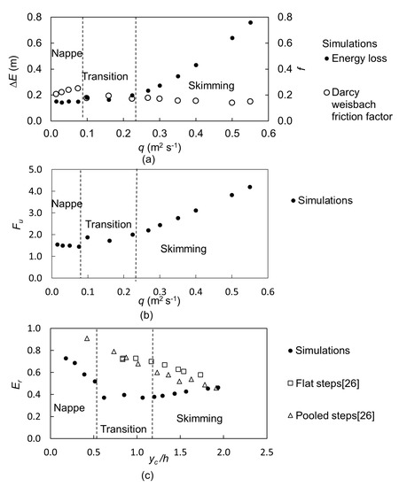
Figure 9.
Effect of flow rate in three flow regimes on (a) energy loss and Darcy Weisbach friction factor; (b) Froude number at upstream section and (c) relative energy loss.
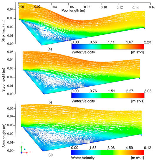
Figure 10.
Circulations in step-pool 2: (a) Transition flow (q = 0.16 m2 s−1); (b) skimming flow. (q = 0.268 m2 s−1); (c) skimming flow (q = 0.55 m2 s−1).
The relationship between, relative energy loss Er and yc/h between upstream and downstream sections is shown in Figure 9c. In nappe flow, Er decreased although energy loss due to step-pool was nearly constant. This is because the total energy at the crest of the step-pool increased for the nappe regime. For transition and skimming flow, Er increased marginally from 0.39 to 0.46 (Figure 9c). For transition and skimming regimes, total energy at the upstream section and energy loss varied from 0.41 m to 1.63 m, and from 0.16 m to 0.76 m, respectively. In the skimming flow regime, in the study reported by Felder [25], Er decreased from 0.73 to 0.58 for flat steps and from 0.60 to 0.49 for pooled steps. The reason for this difference in behavior could be due to difference in geometrical configuration in Felder [25] as compared to the present study. Water pooling was created in the study by Felder [25] using end sills whereas in this study the pool was created with horizontal and vertical slopes as shown in Figure 4.
The values of relative energy loss for nappe flows were compared with values obtained using the empirical model proposed by Agostino and Michelini [27]. The empirical model was developed for only nappe flows and the relative energy loss was expressed as a function of only relative pool depth. Estimated relative energy loss values from Agostino and Michelini [27] model were 0.414, 0.411, 0.400 and 0.370 whereas the simulated results were 0.280, 0.276, 0.300 and 0.201 for relative pool depth of 0.863, 0.874, 0.910 and 1.050, respectively. Relative pool depth was defined as the ratio of water depth in the pool to step height. The comparison indicated an average difference of 34% in the values. This difference was expected because the field investigations of Agostino and Michelini [27] having irregular sized boulders lumped all the effects of all the parameters other than the relative pool depth into the empirical coefficient and exponent. Present simulations do not include the effect of geometric variations in the transverse direction.
3.2. Effect of Horizontal and Vertical Face Inclinations
Numerical experiments were conducted to investigate the effects of horizontal and vertical face inclinations on the energy loss due to step-pools, while keeping other conditions (length of step = 0.77 m, height of step = 0.162 m, flow rate = 0.224 m2 s−1) constant (Table 4). Even though horizontal and vertical face inclinations are changed, the values of h and l were chosen in such a way that the ratio is always 0.21 (Table 4). First, variation in the energy loss was studied by keeping vertical face inclination constant and varying the horizontal face inclination. Energy loss increased by 10.8%, 31.3% and 52.7% as the horizontal face inclination varied from 2° to 10° (Figure 11a), for the inclination of vertical face, = 40° (scenario 1), 55° (scenario 2) and 70° (scenario 3), respectively. Darcy Weisbach friction factor increased from horizontal face inclination 2° to 5° and decreased from 5° to 10° (Figure 11a). Reason for this fluctuation is not known at this juncture and needs to be explored with further investigation. An increase in horizontal face inclination resulted in an increase in the size of the circulation zone in the pool (Figure 12) and also an increase in the spatial extent in the pool where the vorticity is significant, i.e., 30 s−1 (Figure S4). This has increased the energy loss. Similar observations were made in the experimental work carried out by Chinnarasri and Wongwises [19] for stepped chutes, where the angle of inclination of the horizontal face was varied from 10° to 30° and the angle of inclination of the vertical face was zero. It may be noted that the horizontal inclination for step-pools in mountain streams usually varies between 2° and 10°. Moreover, slope of chute in the study conducted by Chinnarasri and Wongwises [19] varied from 30° to 60°, whereas the slope of step-pools mostly varied from 2.9° to 11.4° in nature [27]. Therefore, the present numerical experimental runs added to our understanding of the effects of horizontal and vertical faces on the energy loss in channels with milder bed slopes.
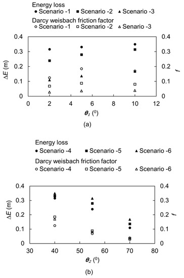
Figure 11.
Effect of horizontal and vertical face inclinations on energy loss and Darcy Weisbach friction factor: (a) Effect of (b) effect of .
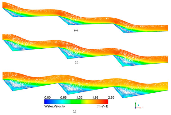
Figure 12.
Velocity vectors on central vertical plane for step-pools: (a) = 2°, = 40°; (b) = 5°, = 40°; and (c) = 10°, = 40°.
Variation in the energy loss was then studied by keeping horizontal face inclination constant and varying the vertical face inclination from 40° to 70°. The same numerical simulations which have been used in the previous section are rearranged here to delineate the effect of vertical face inclination as shown in Figure 12b. Energy loss decreased by 65.1%, 58.5% and 52.2% as the vertical face inclination was varied from 40° to 70° (Figure 11b), for the inclination of horizontal face, = 2° (scenario 4), 5° (scenario 5) and 10° (scenario 6), respectively. Darcy Weisbach friction factor decreased by 75%, while vertical face inclination increased from 40° to 70° (Figure 11b). When vertical face inclination ( increases, energy loss and Darcy Weisbach friction factor decrease because an increase in leads to a flatter vertical face, thereby the water flows smoothly from the crest of the step to the bottom of the pool and recirculation disappears as shown in Figure 13. This is corroborated by the fact that the vorticity decreased from 30 s−1 (Figure S5a) to 6 s−1 (Figure S5c) as the vertical face inclination increased. It is also very clear from Figure S5 that there has been a significant reduction in the spatial extent over which vorticity is more than 6 s−1.
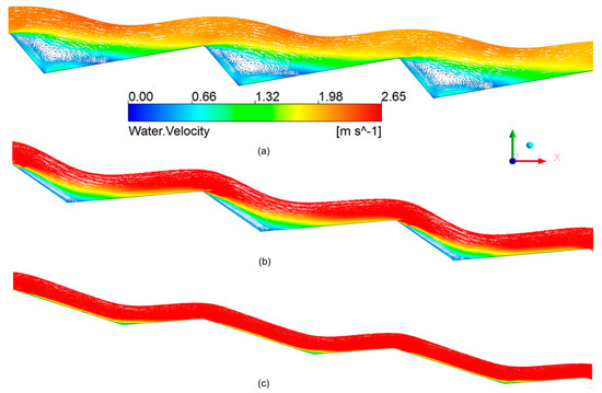
Figure 13.
Velocity vectors on central vertical plane for step-pools: (a) = 10°, = 40°; (b) = 10°, = 55°; and (c) = 10°, = 70°.
3.3. Multiple Step-Pools
In nature, there can be multiple step-pools, occurring in a sequence. It is important to study the variation in energy loss from the first step-pool to the last step-pool, because of the interaction effect of step-pools. In this section, energy loss variation in step-pools 1–3 was investigated when flow was nappe, transition and skimming. In these simulations, length (l), height (h), horizontal face inclination (), vertical face inclination () and slope of sequence of step-pools were kept constant as 0.77 m, 0.162 m, 10°, 40° and 7.7°, respectively.
In nappe flow (q = 0.015 m2 s−1), the difference in energy loss induced by each individual step-pool was not significant. Energy losses in step-pools 1–3 were 0.048 m, 0.047 m and 0.046 m, (5% difference), respectively (Figure 14). The total energy loss for the combination of three step-pools was 0.142 m, which is almost equal to three times the energy loss in an individual step-pool, i.e., the energy loss increases linearly with the number of step-pools in a given reach if the flow regime is nappe flow. For transition flow (q = 0.16 m2 s−1), energy losses in step-pools 1–3 were 0.066 m, 0.059 m and 0.054 m, (18% difference), respectively (Figure 13). While there is a gradual decrease in the energy loss in the downstream step-pools, this decrease is not significant. Total energy loss for all the three steps combined is equal to 0.180 m, which is equal to three times the energy loss in the central step. Here also, one can assume that the energy loss varies more or less linearly with the number of step-pools in a reach. It was observed that upstream Froude numbers (Fu = 1.5) at crests of all step-pools was almost constant for nappe and transition flows. Spatial variation of velocity vectors on the central vertical plane for step-pools 1–3 are similar as shown in Figure 6a,b for nappe and transition flows, respectively. It can be concluded that each step-pool acted as an individual unit, and flow patterns in all the three step-pools were similar.
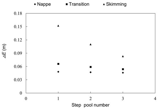
Figure 14.
Spatial variation in energy loss in different flow regimes.
In skimming flow (q = 0.55 m2 s−1), Figure 14 shows that energy loss induced in step-pools 1–3 are 0.152 m, 0.110 m and 0.083 m, respectively. This shows a significant spatial variation (40%) in energy loss. Total energy loss for all the three step-pools was 0.34 m, which is significantly lesser than the energy loss in first step-pool multiplied by 3. This spatial variation in energy loss occurs because the flow in step-pool 1 affects flow in step-pool 2, which in turn affects the flow in step-pool 3. It is noted from Figure 6c that the depth averaged flow velocity and depth at crest of step-pools 1–3 are 4.56 m s−1, 3.63 m s−1, 3.44 m s−1 and 0.12 m, 0.15 m, 0.16 m, respectively. It is interesting to note that Chinnarasri and Wongwises [19] also observed exponential relation between relative energy loss and number of steps for skimming flow, in the context of stepped spillways.
In this paragraph, results presented in the above sections are discussed in the overall context of energy loss in mountainous channels. A simple empirical equation for head loss in steep mountainous channels with step-pools is needed for the development of appropriate hydrodynamic models for these channels. While many previous studies have dealt with quantifying head loss in stepped spillways, only few studies [27] have dealt with head loss in steep natural channels with step-pool formation. However, flow structure in natural channels with step-pools will be different from that in flows over stepped spillways because (i) typical slopes of natural channels are smaller than those adopted for stepped spillways and (ii) the pooling of water in natural channels could occur due to inclination of both vertical and horizontal faces. Numerical experimental results presented in this study clearly demonstrate that the inclinations of vertical and horizontal faces affect the flow structure and the vorticity of flow in the water pool and thus the energy loss. Moreover, earlier empirical equation for head loss in natural channels with step-pools [27] was mostly based on the field data for nappe flow regime. Numerical experimental results presented in this study demonstrate that the flow structure and the vorticity of flow in the water pool are significantly different for a skimming flow as compared to that for a nappe flow. This in turn affects the way head loss occurs in a skimming flow as compared to that in a nappe flow. Earlier empirical equations for head loss in natural step-pool channels considered only relative pool depth as the affecting parameter.
As mentioned earlier, Darcy Weisbach friction factor (f) is calculated using the energy loss, average flow depth, velocity and length of step-pool 2 for the 21 numerical runs. The respective horizontal and vertical face inclinations and Froude numbers along with Darcy Weisbach friction factor is tabulated in Supplementary Table S1. The data is used to develop a simple empirical power law equation as shown below with R2 value of 0.87. The power law was found to be the most reasonable functional relation while studying flow resistance [31,35]. Authors did not consider ratio of step height to length since it is not investigated in this study.
It can be seen from Equation (16), Figure 9a,b and Figure 11b that Froude number at the upstream section and vertical face inclination have negative correlation with the Darcy Weisabch friction factor, while horizontal face inclination has positive correlation. However, this study used a limited number of numerical data to develop the equation and further extensive simulated data is necessary to illustrate the equation in a better way.
Present numerical experimental results also showed that the cumulative energy loss in a channel with a sequence of step-pools is linearly dependent on the number of step-pools for nappe and transition flows, while it is a non-linear function in the case of skimming flows. This observation is useful from the perspective of making field measurements for energy loss. It can be concluded that when a sequence of step-pools exist in the field, one needs to collect energy loss data for only one step-pool when flow is either nappe or transition, provided all step-pools are more or less similar geometrically. However, for skimming flows, energy loss data needs to be collected from all the step-pools in order to gain insight into the interactive effect.
4. Conclusions
Systematic hydrodynamic model studies have been carried out to gain insight into how flow rate and geometric parameters affect the macroscopic flow structure and thus the energy loss in step-pool channels. While an equation for energy loss in mountainous channels is not proposed in this work, results presented here will help to develop an empirical equation for energy loss. The following conclusions are derived from the present study:
- (i)
- For a given step-pool channel, three distinct flow regimes: Nappe, transition and skimming, could be identified as the flow rate increased from low to high.
- (ii)
- In the numerical experiments conducted for nappe flow, the energy loss decreased as the flow rate increased. However, this decrease is marginal and the energy loss was more or less constant at 0.15 m. Energy loss increased from 0.18 m to 0.55 m while the flow regime changed from transition to skimming.
- (iii)
- Darcy Weisbach friction factor high at low flow rate (0.015 m2 s−1 to 0.075 m2 s−1) and decreased at higher flow rates (0.075 m2 s−1 to 0.55 m2 s−1) in step-pool system.
- (iv)
- Energy loss in step-pools is positively correlated with the size of recirculation zone, velocity in the recirculation zone, vorticity and the spatial extent over which the vorticity is high.
- (v)
- When horizontal face inclination was increased from 2° to 10°, energy loss increased by 31.6% and Darcy Weisbach friction factor fluctuated; further investigation is required to understand this behavior.
- (vi)
- When vertical step inclination was increased from 40° to 70°, energy loss and Darcy Weisbach friction factor decreased by 58.6% and 75%, respectively.
- (vii)
- The behavior of step-pool sequence for nappe and transition flow regimes was markedly different from that for skimming flow regime. Energy loss is linearly related to the number of step-pools for nappe and transition flows, whereas it is a nonlinear function for skimming flows.
Supplementary Materials
The following are available online at https://www.mdpi.com/2073-4441/13/1/72/s1, Figure S1: Mesh details: (a) for complete geometry; (b) near the bottom of channel, Figure S2: Vorticity contours for Figure 8: (a) nappe flow (q = 0.015 m2 s−1); (b) nappe flow (q = 0.03 m2 s−1); (c) nappe flow (q = 0.075 m2 s−1) on verge of transition flow, Figure S3: Vorticity contours for Figure 10: (a) transition flow (q = 0.16 m2 s−1); (b) skimming flow (q = 0.268 m2 s−1); (c) skimming flow (q = 0.55 m2 s−1), Figure S4: Vorticity contours for Figure 12: (a) = 2°, = 40°; (b) = 5°, = 40° and (c) = 10°, = 40°, Figure S5: Vorticity contours for Figure 13: (a) = 10°, = 40°; (b) = 10°, = 55° and (c) = 10°, = 70°. Table S1: Numerical data used for empirical equation development.
Author Contributions
S.K.T. contributed to the conceptualization of the problem and carried out the simulations, data analysis and preparation of the draft manuscript. S.M.B. contributed to the conceptualization of the problem, analysis of the data and refinement of the manuscript. The ANSYS-CFX software license was obtained from his institute. P.F., A.B.M.B. and V.C. contributed to the conceptualization of the problem, analysis of the data and refinement of the manuscript. All authors have read and agreed to the published version of the manuscript.
Funding
This work was funded by the Department of Science and Technology, India under grant No. DST/CCP/PR-21/2012 (C) and by the German Academic Exchange Service (DAAD) on behalf of the German Federal Ministry of Education and Research (BMBF) for the visit of Peter Fiener to Indo-German Center for Sustainability at IIT Madras.
Data Availability Statement
The data presented in this study are available in supplementary material.
Acknowledgments
We acknowledge financial support from the Indo-German Centre for Sustainability (IGCS) funded by the Department of Science and Technology, India, through the Indian Institute of Technology Madras and German Academic Exchange Service (DAAD) on behalf of the German Federal Ministry of Education and Research (BMBF).
Conflicts of Interest
The authors declare no conflict of interest.
References
- Alonso, R.L.; Fernández, J.B.; Cugat, M.À.C. Flow resistance equations for mountain rivers. Investig. Agrar. Sist. Recur. For. 2009, 18, 81–91. [Google Scholar]
- Chin, A. The geomorphic significance of step-pools in mountain streams. Geomorphology 2003, 55, 125–137. [Google Scholar] [CrossRef]
- Kumar, R.; Devi, K.R. Conservation of freshwater habitats and fishes in the Western Ghats of India. Int. Zoo Yearb. 2013, 47, 71–80. [Google Scholar] [CrossRef]
- Maloney, K.O.; Munguia, P.; Mitchell, R.M. Anthropogenic disturbance and landscape patterns affect diversity patterns of aquatic benthic macroinvertebrates. J. N. Am. Benthol. Soc. 2011, 30, 284–295. [Google Scholar] [CrossRef]
- Yochum, S.E.; Bledsoe, B.P.; David, G.C.L.; Wohl, E. Velocity prediction in high-gradient channels. J. Hydrol. 2012, 424–425, 84–98. [Google Scholar] [CrossRef]
- Campisano, A.; Creaco, E.; Modica, C. Nondimensional simulation-based regression formulas for slit dam design in mountain rivers. J. Hydraul. Eng. 2018, 144, 1–10. [Google Scholar] [CrossRef]
- Comiti, F.; Mao, L.; Wilcox, A.; Wohl, E.E.; Lenzi, M.A. Field-derived relationships for flow velocity and resistance in high-gradient streams. J. Hydrol. 2007, 340, 48–62. [Google Scholar] [CrossRef]
- Nickolotsky, A.; Pavlowsky, R.T. Morphology of step-pools in a wilderness headwater stream: The importance of standardizing geomorphic measurements. Geomorphology 2007, 83, 294–306. [Google Scholar] [CrossRef]
- Chin, A.; Phillips, J.D. The self-organization of step-pools in mountain streams. Geomorphology 2007, 83, 346–358. [Google Scholar] [CrossRef]
- Recking, A.; Leduc, P.; LieBault, F.; Church, M. A field investigation of the influence of sediment supply on step-pool morphology and stability. Geomorphology 2012, 139–140, 53–66. [Google Scholar] [CrossRef]
- Chartrand, S.M.; Jellinek, M.; Whiting, P.J.; Stamm, J. Geometric scaling of step-pools in mountain streams: Observations and implications. Geomorphology 2011, 129, 141–151. [Google Scholar] [CrossRef]
- Thomas, D.B.; Abt, S.R.; Mussetter, R.A.; Harvey, M.D. A design procedure for sizing step-pool structures. In Proceedings of the Joint Conference on Water Resource Engineering and Water Resources Planning and Management: Building Partenships 2000, Minneapollis, MN, USA, 30 July–2 August 2000. [Google Scholar]
- Zhao-Yin, W.; Charles, S.M.; Xue-Hua, D.; Guo-An, Y. Ecological and hydraulic studies of step-pool systems. J. Hydraul. Eng. 2009, 135, 705–717. [Google Scholar]
- Kalathil, S.T.; Chandra, V. Review of step-pool hydro dynamics in mountain streams. Prog. Phys. Geog. 2019, 43, 607–626. [Google Scholar] [CrossRef]
- Maxwell, A.R.; Papanicolaou, A.N. Geometric characteristics of step-pool streams. In Proceedings of the Joint Conference on Water Resource Engineering and Water Resources Planning and Management: Building Partenships 2000, Minneapollis, MN, USA, 30 July–2 August 2000. [Google Scholar]
- Peterson, D.F.; Mohanty, P.K. Flume studies of flow in steep, rough channels. J. Hydraul. Div. 1960, 86, 55–76. [Google Scholar]
- Sindelar, C.; Smart, G. Transition flow in step pool system: Pressure distribution and drag forces. J. Hydraul. Eng. 2016, 142, 683–688. [Google Scholar] [CrossRef]
- Toombes, L. Experimental study of air-water flow properties on low-gradient stepped cascades. Ph.D. Thesis, University of Queensland, Australia, Brisbane, 2002. [Google Scholar]
- Chinnarasri, C.; Wongwises, S. Flow patterns and energy dissipation over various stepped chutes. J. Irrig. Drain. Eng. 2006, 132, 70–76. [Google Scholar] [CrossRef]
- Pagliara, S.; Dazzini, D. Hydraulics of block ramp for river restoration. In Proceedings of the 2nd International Conference on New Trends in Water and Environmental Engineering for Safety and Life: Eco-compatible Solution for Aquatic Environments 2002, Capri, Italy, 24–28 June 2002; pp. 165–166. [Google Scholar]
- David, G.C.L.; Wohl, E.; Yochum., S.E.; Bledsoe, B.P. Controls on spatial variations in flow resistance along steep mountain streams. Water Resour. Res. 2010, 46, 1–21. [Google Scholar] [CrossRef]
- Kaufmann, P.R.; Faustini, J.M.; Larsen, D.P.; Shirazi, M.A. A roughness-corrected index of relative bed stability for regional stream surveys. Geomorphology 2008, 99, 150–170. [Google Scholar] [CrossRef]
- Lee, A.J.; Ferguson, R.I. Velocity and flow resistance in step-pool streams. Geomorphology 2002, 46, 59–71. [Google Scholar] [CrossRef]
- Comiti, F.; Cadol, D.; Wohl, E. Flow regimes, bed morphology, and flow resistance in self-formed step-pool channels. Water Resour. Res. 2009, 45, 1–18. [Google Scholar] [CrossRef]
- Felder, S. Air-Water Flow Properties on Stepped Spillways for Embankment Dams: Aeration, Energy Dissipation and Turbulence on Uniform, Non-Uniform and Pooled Stepped Chutes. Ph.D. Thesis, University of Queensland, Brisbane, Australia, 2013. [Google Scholar]
- Felder, S.; Fromm, C.; Chanson, H. Air Entrainment and Energy Dissipation on a 8.9 Slope Stepped Spillway with Flat and Pooled Steps; University of Queensland: Brisbane, Australia, 2012. [Google Scholar]
- Agostino, V.D.; Michelini, T. On kinematics and flow velocity prediction in step-pool channels. Water Resour. Res. 2015, 51, 4650–4667. [Google Scholar] [CrossRef]
- Andre, S. High Velocity Aerated Flows on Stepped Chutes with Macro-Roughness Elements. Ph.D. Thesis, Swiss Federal Institute of Technology Lausanne, Lausanne, Switzerland, 2004. [Google Scholar]
- Nikseresht, A.H.; Talebbeydokhti, N.; Rezaei, M.J. Numerical simulation of two-phase flow on step-pool spillways. Sci. Iran. 2013, 20, 222–230. [Google Scholar]
- Peyras, L.; Royet, P.; Degoutte, G. Flow and energy dissipation over stepped gabion weirs. J. Hydraul. Eng. 1992, 118, 707–717. [Google Scholar] [CrossRef]
- Baki, A.B.M.; Zhu, D.Z.; Rajaratnam, N. Flow simulation in a rock-ramp fish pass. J. Hydraul. Eng. 2016, 142, 04016031. [Google Scholar] [CrossRef]
- Baki, A.B.M.; Zhu, D.Z.; Harwood, A.; Lewis, A.; Healey, K. Rock-weir fishway I: Flow regimes and hydraulic characteristics. J. Ecohydraul. 2017, 2, 122–141. [Google Scholar] [CrossRef]
- Marriner, B.A.; Baki, A.B.M.; Zhu, D.Z.; Thiem, J.D.; Cooke, S.J.; Katopodis, C. Field and numerical assessment of turning pool hydraulics in a vertical slot fishway. Ecol. Eng. 2014, 63, 88–101. [Google Scholar] [CrossRef]
- Salaheldin, T.M.; Imran, J.; Chaudhry, M.H. Numerical modeling of three-dimensional flow field around circular piers. J. Hydraul. Eng. 2004, 130, 91–100. [Google Scholar] [CrossRef]
- Thappeta, S.K.; Bhallamudi, S.M.; Fiener, P.; Narasimhan, B. Resistance in steep open channels due to randomly distributed macro roughness elements at large Froude numbers. J. Hydrol. Eng. 2017, 22, 1–15. [Google Scholar] [CrossRef]
- Chen, Q.; Dai, G.; Liu, H. Volume of fluid model for turbulence numerical simulation of stepped spillway overflow. J. Hydraul. Eng. 2002, 128, 683–688. [Google Scholar] [CrossRef]
- Heidari, A.; Ghasemi, P. Evaluation of step’s slope on energy dissipation in stepped spillway. Int. J. Eng. Technol. 2014, 3, 501. [Google Scholar] [CrossRef][Green Version]
- Chiu, C.L.; Fan, C.M.; Tsung, S.C. Numerical modeling for periodic oscillation of free over fall in a vertical drop pool. J. Hydraul. Eng. 2016, 143, 04016077. [Google Scholar] [CrossRef]
- Bombardelli, F.A.; Meireles, I.; Matos, J. Laboratory measurements and multi-block numerical simulations of the mean flow and turbulence in the non-aerated skimming flow region of steep stepped spillways. Environ. Fluid Mech. 2011, 11, 263–288. [Google Scholar] [CrossRef]
- Morovati, K.H.; Eghbalzadeh, A. Study of inception point, void fraction and pressure over pooled stepped spillways using FLOW-3D. Int. J. Numer. Methods Heat Fluid Flow 2018, 28, 982–998. [Google Scholar] [CrossRef]
- Bayon, A.; Valero, D.; Garcia-Bartual, R.; Valles-Moran, F.J.; Lopez-Jimenez, P.A. Performance assessment of OpenFOAM and FLOW-3D in the numerical modeling of a low Reynolds number hydraulic jump. Environ. Model. Softw. 2016, 80, 322–335. [Google Scholar] [CrossRef]
- Valero, D.; Bung, D.B.; Crookston, B.M. Energy dissipation of a Type III basin under design and adverse conditions for stepped and smooth spillways. J. Hydraul. Eng. 2018, 144, 04018036. [Google Scholar] [CrossRef]
- Abdulla, A.A. Three-Dimensional Flow Model for Different Cross-Section High-Velocity Channels. Ph.D. Thesis, University of Plymouth, Plymouth, UK, 2013. [Google Scholar]
- Spalart, P.R.; Shur, M. On the sensitization of turbulence model to rotation and curvature. Aerosp. Sci. Tech. 1997, 1, 297–302. [Google Scholar] [CrossRef]
- ANSYS-CFX. Solver Theory Guide; ANSYS: Canonsburg, PA, USA, 2014. [Google Scholar]
- Jone, W.P.; Launder, B.E. The prediction of laminarization with a two-equation model of turbulence. Int. J. Heat Mass Transf. 1972, 15, 301–314. [Google Scholar] [CrossRef]
- Hirt, C.W.; Nichols, B.D. Volume of fluid (VOF) method for the dynamics of free boundaries. J. Comput. Phys. 1981, 39, 201–225. [Google Scholar] [CrossRef]
- Castillo, L.G.; Carrillo, J.M.; García, J.T.; Vigueras-Rodríguez, A. Numerical simulations and laboratory measurements in hydraulic jumps. In Proceedings of the 11th International Conference on Hydroinformatics 2014, New York, NY, USA, 17–21 August 2014. [Google Scholar]
- Xiang, M.; Cheung, S.C.P.; Tu, J.Y.; Zhang, W.H. A multi-fluid modelling approach for the air entrainment and internal bubbly flow region in hydraulic jumps. Ocean Eng. 2014, 91, 51–63. [Google Scholar] [CrossRef]
- Israngkura, U.; Chinnarasri, C. Flow depth and energy losses through stepped chutes. In Proceedings of the 9th Congress of the Asian and Pacific Division of the International Association for Hydraulic Research 1994, Singapore, 24–26 August 1994; pp. 156–163. [Google Scholar]


Publisher’s Note: MDPI stays neutral with regard to jurisdictional claims in published maps and institutional affiliations. |
© 2020 by the authors. Licensee MDPI, Basel, Switzerland. This article is an open access article distributed under the terms and conditions of the Creative Commons Attribution (CC BY) license (http://creativecommons.org/licenses/by/4.0/).