A Semi-Theoretical Model for Water Condensation: Dew Used in Conservation of Earthen Heritage Sites


Abstract
1. Introduction
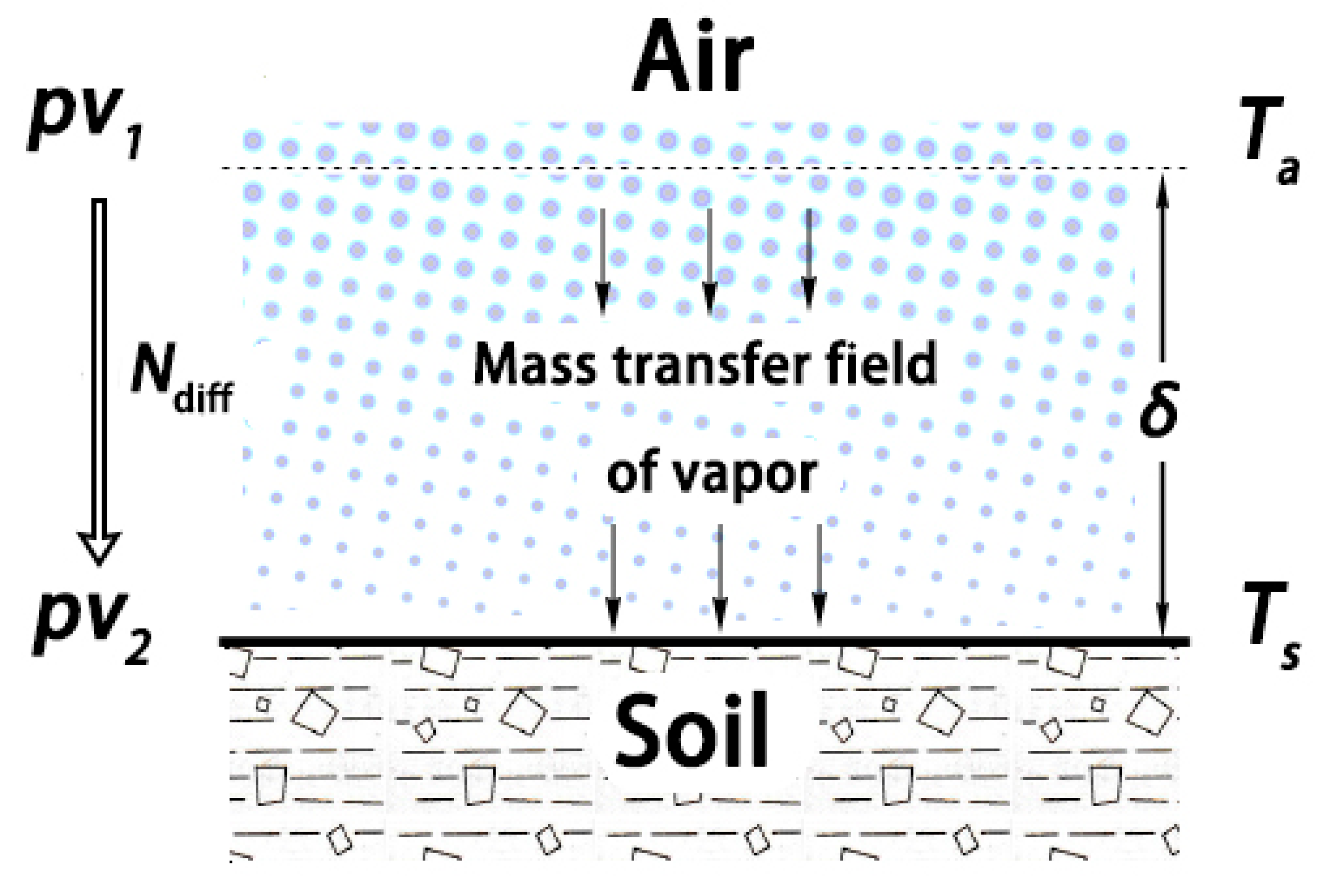
2. Theory
3. Materials and Methods
3.1. Data Collection
3.1.1. Laboratory Experiments
3.1.2. Field Experiments in the Kuahuqiao Museum
3.1.3. Field Experiments in a Desert System
3.2. Calculations
3.2.1. Simulations Using the Semi-Theoretical Model
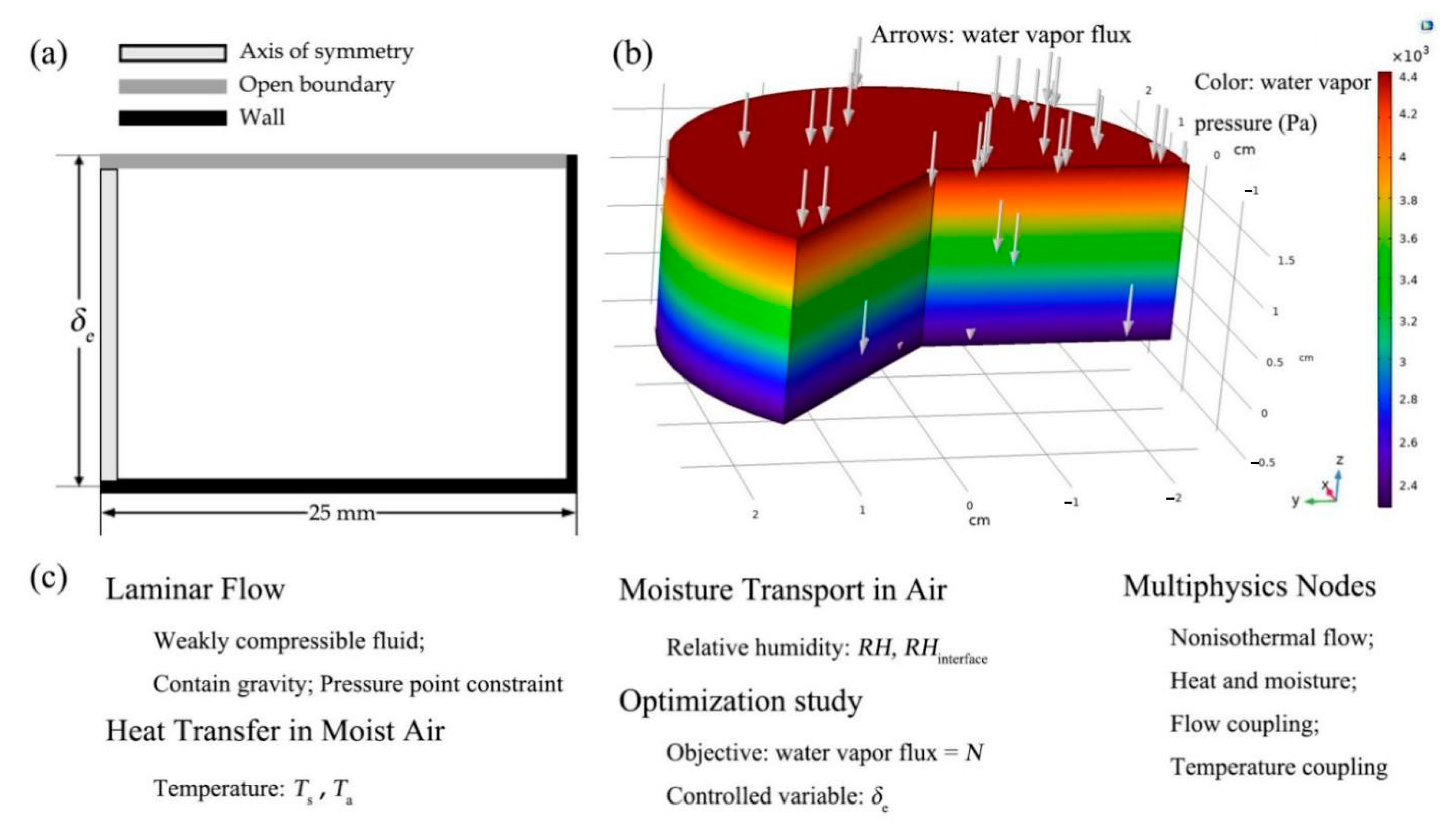
3.2.2. Numerical Simulations of Laboratory Experiments
4. Results
4.1. Laboratory Experiments and Numerical Simulations
4.2. Field Experiments at the Kuahuqiao Site Museum
4.3. Field Experiments in a Desert System
5. Discussions
5.1. Model Validation Using Numerical Simulation
5.2. Application Potential and Unexplained Parameters
6. Conclusions
Supplementary Materials
Author Contributions
Funding
Institutional Review Board Statement
Informed Consent Statement
Data Availability Statement
Acknowledgments
Conflicts of Interest
References
- Algarni, S.; Saleel, C.; Mujeebu, M.A. Air-conditioning condensate recovery and applications—Current developments and challenges ahead. Sustain. Cities Soc. 2018, 37, 263–274. [Google Scholar] [CrossRef]
- Tomaszkiewicz, M.; Najm, M.A.; Beysens, D.; Alameddine, I.; El-Fadel, M. Dew as a sustainable non-conventional water resource: A critical review. Environ. Rev. 2015, 23, 425–442. [Google Scholar] [CrossRef]
- Tomaszkiewicz, M.; Najm, M.A.; Zurayk, R.; El-Fadel, M. Dew as an adaptation measure to meet water demand in agriculture and reforestation. Agric. For. Meteorol. 2017, 232, 411–421. [Google Scholar] [CrossRef]
- Kim, H.; Rao, S.R.; Kapustin, E.A.; Zhao, L.; Yang, S.; Yaghi, O.M.; Wang, E.N. Adsorption-based atmospheric water harvesting device for arid climates. Nat. Commun. 2018, 9, 1–8. [Google Scholar] [CrossRef]
- Wang, X.-S.; Wan, L.; Huang, J.; Cao, W.; Xu, F.; Dong, P. Variable temperature and moisture conditions in Yungang Grottoes, China, and their impacts on ancient sculptures. Environ. Earth Sci. 2014, 72, 3079–3088. [Google Scholar] [CrossRef]
- Shen, Y.-X.; Chen, W.; Kuang, J.; Du, W.-F. Effect of salts on earthen materials deterioration after humidity cycling. J. Cent. South Univ. 2017, 24, 796–806. [Google Scholar] [CrossRef]
- Sterflinger, K.; Pinzari, F. The revenge of time: Fungal deterioration of cultural heritage with particular reference to books, paper and parchment. Environ. Microbiol. 2011, 14, 559–566. [Google Scholar] [CrossRef]
- Parracha, J.L.; Pereira, A.S.; da Silva, R.V.; Almeida, N.; Faria, P. Efficacy of iron-based bioproducts as surface biotreatment for earth-based plastering mortars. J. Clean. Prod. 2019, 237. [Google Scholar] [CrossRef]
- Li, L.; Shao, M.; Wang, S.; Li, Z. Preservation of earthen heritage sites on the Silk Road, northwest China from the impact of the environment. Environ. Earth Sci. 2010, 64, 1625–1639. [Google Scholar] [CrossRef]
- Zhang, H.; Hu, T.; Huang, X.; Wang, J.; Jiang, H.; Zhang, S. Hydrophilic organosilicone rubber: The new organic-inorganic hybrid consolidant for ancient earthen architectures. Intern. J. Conserv. Sci. 2015, 6, 35–44. [Google Scholar]
- García-Vera, V.E.; Tenza-Abril, A.J.; Lanzón, M. The effectiveness of ethyl silicate as consolidating and protective coating to extend the durability of earthen plasters. Constr. Build. Mater. 2020, 236, 117445. [Google Scholar] [CrossRef]
- García-Vera, V.E.; Tenza-Abril, A.J.; García-Vera, V.; Lanzón, M. Calcium hydroxide nanoparticles coatings applied on cultural heritage materials: Their influence on physical characteristics of earthen plasters. Appl. Surf. Sci. 2020, 504, 144195. [Google Scholar] [CrossRef]
- Chiari, G. Chemical surface treatments and capping techniques of earthen structures: A long term evaluation. In Proceedings of the 6th International Conference on the Conservation of Earthen Architectures—Plenary Lecture, Las Cruces, NM, USA, 14–19 October 1990; pp. 267–273. [Google Scholar]
- Zhang, C.; Zhang, B.; Cui, B. High hydrophobic preservation materials can cause damage to tabia relics. Prog. Org. Coatings 2020, 145, 105683. [Google Scholar] [CrossRef]
- Xu, Y.; Wang, S.; Zhang, B.; Wu, J. Investigation and research on relics diseases of the earthen site of Kuahuqiao Site Museum. Sci. Conserv. Archaeol. 2018, 1, 53–62, (In Chinese with English abstract). [Google Scholar]
- Wang, S.; Zhang, B.; Wu, J. Study on the feasibility of replenishment for soil sites in museum environment by phase transition. Sci. Conserv. Archaeol. 2019, 3, 16–25, (In Chinese with English abstract). [Google Scholar] [CrossRef]
- Correia, M.; Guerrero, L.; Crosby, A. Technical Strategies for Conservation of Earthen Archaeological Architecture. Conserv. Manag. Archaeol. Sites 2015, 17, 224–256. [Google Scholar] [CrossRef]
- Jacobs, A.F.G.; Heusinkveld, B.G.; Berkowicz, S.M. Force-restore technique for ground surface temperature and moisture content in a dry desert system. Water Resour. Res. 2000, 36, 1261–1268. [Google Scholar] [CrossRef]
- Jacobs, A.F.; Heusinkveld, B.G.; Berkowicz, S.M. Dew deposition and drying in a desert system: A simple simulation model. J. Arid. Environ. 1999, 42, 211–222. [Google Scholar] [CrossRef]
- Camuffo, D.; Giorio, R. Quantitative Evaluation of Water Deposited By Dew on Monuments. Boundary-Layer Meteorol. 2003, 107, 655–672. [Google Scholar] [CrossRef]
- Al-Farayedhi, A.A.; Ibrahim, N.I.; Gandhidasan, P. Condensate as a water source from vapor compression systems in hot and humid regions. Desalination 2014, 349, 60–67. [Google Scholar] [CrossRef]
- Allen, R.; Pruitt, W.O.; Wright, J.L.; Howell, T.A.; Ventura, F.; Snyder, R.; Itenfisu, D.; Steduto, P.; Berengena, J.; Yrisarry, J.B.; et al. A recommendation on standardized surface resistance for hourly calculation of reference ETo by the FAO56 Penman-Monteith method. Agric. Water Manag. 2006, 81, 1–22. [Google Scholar] [CrossRef]
- Rui-Hong, Y.; Zhang, Z.; Lu, X.X.; Chang, I.; Liu, T. Variations in dew moisture regimes in desert ecosystems and their influencing factors. Wiley Interdiscip. Rev. Water 2020, 7, e1482. [Google Scholar] [CrossRef]
- Agam, N.; Berliner, P. Dew formation and water vapor adsorption in semi-arid environments—A review. J. Arid. Environ. 2006, 65, 572–590. [Google Scholar] [CrossRef]
- Busscher, W. Simulation of Field Water Use and Crop Yield. Soil Sci. 1980, 129, 193. [Google Scholar] [CrossRef]
- Lier, Q.D.J.V.; van Dam, J.C.; Durigon, A.; dos Santos, M.A.; Metselaar, K. Modeling Water Potentials and Flows in the Soil-Plant System Comparing Hydraulic Resistances and Transpiration Reduction Functions. Vadose Zone J. 2013, 12. [Google Scholar] [CrossRef]
- Mircioiu, C.; Voicu, V.A.; Anuţa, V.; Tudose, A.; Celia, C.; Paolino, D.; Fresta, M.; Sandulovici, R.; Mircioiu, I. Mathematical Modeling of Release Kinetics from Supramolecular Drug Delivery Systems. Pharmaceutics 2019, 11, 140. [Google Scholar] [CrossRef]
- Camillo, P.J.; Gurney, R.J.; Schmugge, T.J. A soil and atmospheric boundary layer model for evapotranspiration and soil moisture studies. Water Resour. Res. 1983, 19, 371–380. [Google Scholar] [CrossRef]
- Fu, X.; Shen, W.; Yao, T.; Hou, W. Physical Chemistry, 5th ed.; Higher Education Press: Beijing, China, 2005; pp. 277–278. [Google Scholar]
- Steiger, M.; Asmussen, S. Crystallization of sodium sulfate phases in porous materials: The phase diagram Na2SO4–H2O and the generation of stress. Geochim. Cosmochim. Acta 2008, 72, 4291–4306. [Google Scholar] [CrossRef]
- Jacobs, A.F.G.; Heusinkveld, B.G.; Berkowicz, S.M. Dew measurements along a longitudinal sand dune transect, Negev Desert, Israel. Int. J. Biometeorol. 2000, 43, 184–190. [Google Scholar] [CrossRef]
- Wu, J. Environmental remediation project of the Kuahuqiao underwater site. Fujian Wenbo. 2015, 4, 35–39. (In Chinese) [Google Scholar]


| Experimental Conditions | Results of Phase I | Results of Phase II | |||||||
|---|---|---|---|---|---|---|---|---|---|
| Relative Humidity | Air Temperature | Interface Temperature | Measured Rate | Simulated Rate | Equivalent Thickness | Measured Rate | Simulated Rate | Equivalent Thickness | |
| RH/% | Ta/°C | Ts/°C | N/kgm−2h−1 | δe/m | N/kgm−2h−1 | δe/m | |||
| 1 | 65.39 | 30.07 | 14.49 | 0.04823 | 0.04616 | 0.02194 | 0.02628 | 0.04402 | 0.03897 |
| 2 | 75.31 | 31.05 | 23.60 | 0.02481 | 0.01977 | 0.02773 | 0.02020 | 0.03003 | 0.03406 |
| 3 | 73.02 | 33.35 | 21.21 | 0.03740 | 0.05025 | 0.03043 | 0.04026 | 0.05000 | 0.02827 |
| 4 | 73.93 | 30.10 | 14.44 | 0.05135 | 0.06127 | 0.02480 | 0.04745 | 0.05432 | 0.02684 |
| 5 | 88.03 | 30.79 | 23.86 | 0.04972 | 0.03862 | 0.02022 | 0.04327 | 0.04299 | 0.02324 |
| 6 | 84.40 | 33.28 | 21.27 | 0.08520 | 0.07286 | 0.01770 | 0.07236 | 0.06547 | 0.02084 |
| 7 | 83.80 | 32.12 | 16.24 | 0.08257 | 0.08853 | 0.02083 | 0.07234 | 0.07390 | 0.02377 |
| 8 | 65.39 | 35.03 | 19.45 | 0.05676 | 0.05857 | 0.02176 | 0.03518 | 0.05499 | 0.03511 |
| 9 | 75.31 | 31.05 | 23.60 | 0.02604 | 0.01977 | 0.02642 | 0.02048 | 0.03003 | 0.03360 |
| 10 | 73.02 | 33.35 | 21.20 | 0.04667 | 0.05031 | 0.02440 | 0.05594 | 0.05004 | 0.02035 |
| 11 | 73.93 | 35.07 | 19.41 | 0.07327 | 0.07882 | 0.02130 | 0.05095 | 0.06881 | 0.03063 |
| 12 | 88.03 | 30.79 | 23.86 | 0.05302 | 0.03862 | 0.01897 | 0.04453 | 0.04299 | 0.02258 |
| 13 | 84.40 | 33.28 | 21.27 | 0.08413 | 0.07286 | 0.01792 | 0.07603 | 0.06547 | 0.01983 |
| 14 | 83.80 | 35.18 | 19.30 | 0.08749 | 0.10341 | 0.02233 | 0.10422 | 0.08557 | 0.01874 |
| 15 | 67.34 | 35.12 | 19.36 | 0.06233 | 0.06436 | 0.02128 | |||
| 16 | 74.79 | 30.96 | 23.70 | 0.02834 | 0.01742 | 0.02297 | |||
| 17 | 75.18 | 33.82 | 20.72 | 0.04340 | 0.06204 | 0.03040 | |||
| 18 | 70.73 | 35.29 | 19.19 | 0.07075 | 0.07474 | 0.02106 | |||
| 19 | 88.10 | 31.34 | 23.29 | 0.05690 | 0.04786 | 0.02013 | |||
| 20 | 84.89 | 33.60 | 20.95 | 0.09055 | 0.07914 | 0.01769 | |||
| 21 | 80.06 | 34.98 | 19.50 | 0.09126 | 0.09149 | 0.01936 | |||
| Fitting parameters | δ = 2.309 × 10⁻² | δ = 2.582 × 10⁻² | |||||||
| a = −10.03 | a = −0.04854 | ||||||||
| Correlation coefficient R | 0.9182 | 0.9028 | |||||||
| Phase I | Phase II | |||
|---|---|---|---|---|
| Equivalent Thickness δe | Fitting Parameter δ | Equivalent Thickness δe | Fitting Parameter δ | |
| M | 0.02236 | 0.02309 | 0.02692 | 0.02582 |
| SD | 1.428 × 10⁻⁵ | 0 | 4.330 × 10⁻⁵ | 0 |
| Df | 20 | 13 | ||
| p | 0.39 | 0.54 | ||
| t | −0.88 | 0.62 | ||
| Laboratory Experiments | Field Experiments in the Kuahuqiao Site | Field Experiments in a Desert System | ||
|---|---|---|---|---|
| Phase I | Phase II | |||
| δ/10−2 | 2.309 | 2.583 | 0.458 | 3.82 |
| a | −10.03 | −0.04854 | 2.91 × 10³ | 1.25 × 10³ |
Publisher’s Note: MDPI stays neutral with regard to jurisdictional claims in published maps and institutional affiliations. |
© 2020 by the authors. Licensee MDPI, Basel, Switzerland. This article is an open access article distributed under the terms and conditions of the Creative Commons Attribution (CC BY) license (http://creativecommons.org/licenses/by/4.0/).
Share and Cite
He, X.; Wang, S.; Zhang, B. A Semi-Theoretical Model for Water Condensation: Dew Used in Conservation of Earthen Heritage Sites. Water 2021, 13, 52. https://doi.org/10.3390/w13010052
He X, Wang S, Zhang B. A Semi-Theoretical Model for Water Condensation: Dew Used in Conservation of Earthen Heritage Sites. Water. 2021; 13(1):52. https://doi.org/10.3390/w13010052
Chicago/Turabian StyleHe, Xiang, Sijia Wang, and Bingjian Zhang. 2021. "A Semi-Theoretical Model for Water Condensation: Dew Used in Conservation of Earthen Heritage Sites" Water 13, no. 1: 52. https://doi.org/10.3390/w13010052
APA StyleHe, X., Wang, S., & Zhang, B. (2021). A Semi-Theoretical Model for Water Condensation: Dew Used in Conservation of Earthen Heritage Sites. Water, 13(1), 52. https://doi.org/10.3390/w13010052