Article

A Simple Time-Varying Sensitivity Analysis (TVSA) for Assessment of Temporal Variability of Hydrological Processes

1
Department of Civil Engineering, Universidad Católica de la Santísima Concepción, Concepción 4090541, Chile
2
Centro de Investigación en Biodiversidad y Ambientes Sustentables CIBAS, Concepción 4090541, Chile
*
Author to whom correspondence should be addressed.
Water 2020, 12(9), 2463; https://doi.org/10.3390/w12092463
Submission received: 25 June 2020 / Revised: 29 August 2020 / Accepted: 31 August 2020 / Published: 2 September 2020
(This article belongs to the Special Issue Assessment of Spatial and Temporal Variability of Water Resources)

Abstract

:
Time-varying sensitivity analysis (TVSA) allows sensitivity in a moving window to be estimated and the time periods in which the specific components of a model can affect its performance to be identified. However, one of the disadvantages of TVSA is its high computational cost, as it estimates sensitivity in a moving window within an analyzed series, performing a series of repetitive calculations. In this article a function to implement a simple TVSA with a low computational cost using regional sensitivity analysis is presented. As an example of its application, an analysis of hydrological model results in daily, monthly, and annual time windows is carried out. The results show that the model allows the time sensitivity of a model with respect to its parameters to be detected, making it a suitable tool for the assessment of temporal variability of processes in models that include time series analysis. In addition, it is observed that the size of the moving window can influence the estimated sensitivity; therefore, analysis of different time windows is recommended.

1. Introduction

Sensitivity analysis studies the impact of input factor variation on model results [1,2]. Its application and understanding have increased in recent years, and it has been recognized as an essential tool for the development and assessment of environmental models [1,3,4,5]. Depending on the objective of the study, sensitivity analysis allows the factors that most (and least) influence the model results to be identified, model behavior to be understood and interpreted, and uncertainty in the results to be reduced, among other benefits [1,2,4,6,7,8,9,10,11]. There are various methods to carry out a sensitivity analysis, the most popular of which are the Fourier Amplitude Sensitivity Test (FAST) [12], Regional Sensitivity Analysis (RSA) [13], the Morris method [14], the method based on Sobol’s variance [6,15], the PAWN method [16], and, most recently, Variogram Analysis of Response Surfaces (VARS) [9,10,17].
The sensitivity of a model to different factors can vary over a time series due to the presence of environmental, hydrological, and climatic variations and processes that act on different time scales [18,19]. Unlike traditional sensitivity analysis, which is based on model aggregation over time, generating a loss of information within the analysis series [18,20], TVSA allows sensitivity in a moving window to be estimated, where the calculated value is assigned to the center of the window, and likewise for the following time step. The advantage of using a moving window is that the estimations are less affected by atypical values in the data, and not doing so could affect the sensitivity of a factor, highlighting it before or after the periods in which it is actually sensitive [18]. Therefore, TVSA aids in identifying the time periods in which the specific components of a model can affect its performance and uses the additional information to analyze the model functioning and obtain a more precise estimate of the factors [18,21]. In addition, TVSA would allow the appropriate model to be selected according to the pursued objective, thereby complementing new calibration approaches such as the stratified calibration shown by Zhao et al. [22], where a recalibration of the parameters under different conditions and periods over the analyzed time series is described.
Examples of existing software that includes time-varying analysis are MCAT [23], SAFE [4], and VARS-TOOL [17]. The first performs an identifiability analysis using the RSA (DYNIA) method, the second using the PAWN, FAST, Sobol, and Morris methods in a moving window, and the third using the Sobol, Morris, and VARS methods via the Generalized Global Sensitivity Matrix (GGSM) [17]. Although these toolboxes were developed to facilitate the application of sensitivity analysis, one of the main drawbacks of TVSA is its high computational cost, as the calculations are made repetitively for each time step. This cost is commonly assessed in terms of the quantity of model evaluations required for the method to generate acceptable results in terms of robustness; it is therefore associated with a high execution time, as well as computer memory requirements that mean that TVSAs in some models with a large number of parameters cannot be run on a regular computer. The computational cost can be larger or smaller depending on the analysis method used; e.g., the required number of evaluations to estimate sensitivity indices using the PAWN [20], Morris [24,25], and Sobol [21,26] methods ranges from 20,000 to 6,000,000. The number of evaluations depends highly on the quantity of model factors (parameters and/or variables) to considered in the analyses [16].
Because the quantity of model evaluations makes this process the most demanding in computational terms, the objective of this article is to propose a novel and simpler (in comparison to existing methods) alternative for implementing a TVSA with a low computational cost. To this end, a TVSA based on the RSA method is proposed, given that it requires fewer evaluations to obtain stable results [2].
As an application example, the 10-parameter Hydrologiska Byråns Vattenbalansavdelning (HBV) hydrological model [27] is evaluated using information from the Allipén River watershed, Chile. In addition, to support the analysis of the results, a comparison with the standardized precipitation index (SPI) is included.

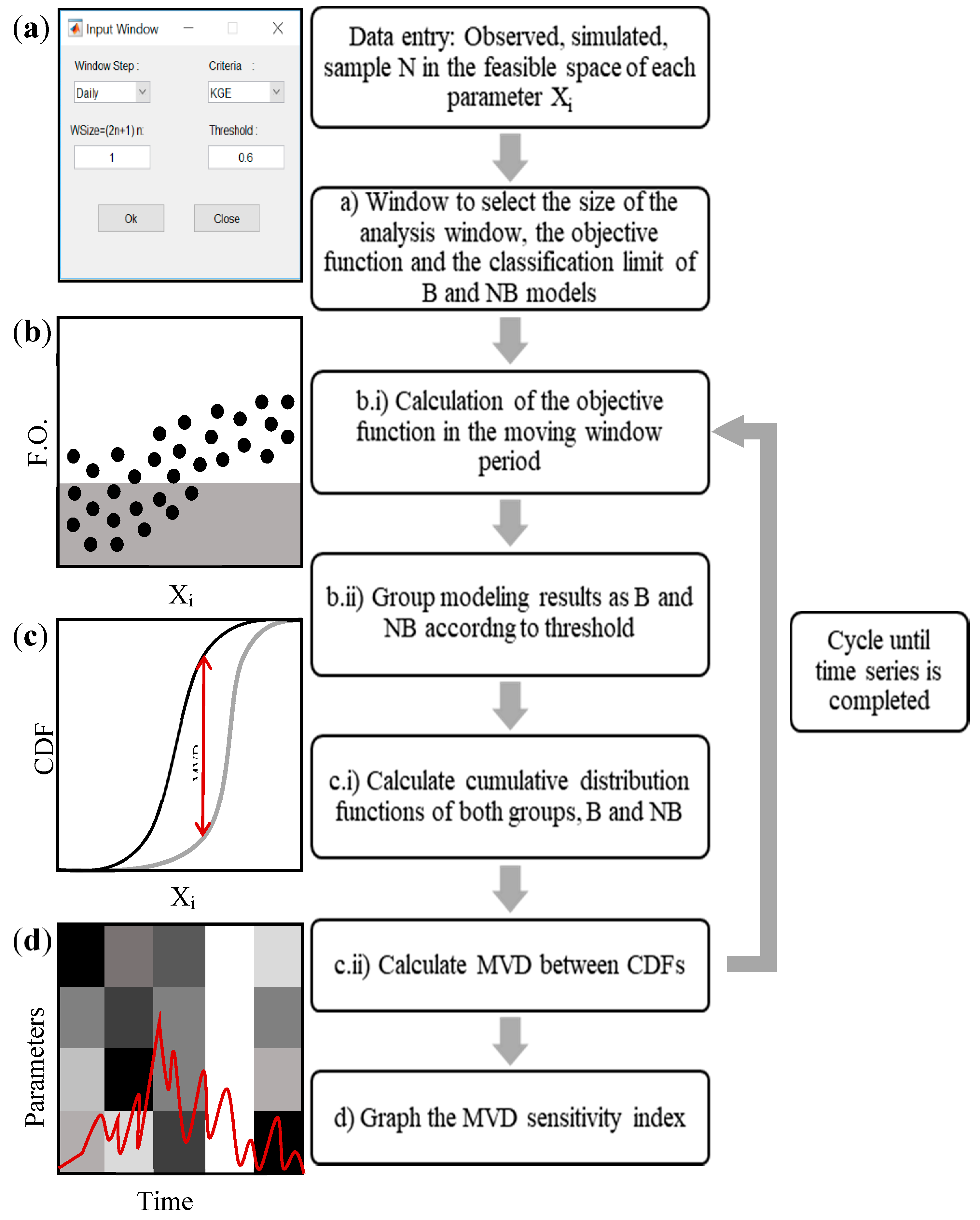
2. TVSA Function Description

The function was designed to evaluate the results of a model through an easy-to-understand, low-computational-resource-consumption TVSA. It was initially developed for hydrological models that simulate daily streamflows; however, it can be modified and used in other environmental models. As Supplementary Material to this paper, a script coded in MATLAB is included. The code includes comments to facilitate its understanding and explain its calculation procedure.
As a TVSA is based on the application of a sensitivity analysis in a moving window instead of the entire evaluation period, its computational cost (i.e., processing, time, and memory cost) is directly related to the computational cost of the sensitive analysis used as a base. Therefore, a TVSA that is simpler and lighter than existing options should be based on a simpler sensitivity analysis, where the convergence and computational costs of which are lower.
The TVSA proposed here is based on RSA. RSA was first proposed and investigated by Spear and Hornberger [13]. The method consists of generating a sample of N points in the feasible space of each parameter, obtained from a previously defined distribution (generally uniform). The parameter sets are grouped into behavioral and nonbehavioral (B and NB, respectively) models based on a performance measure [28,29], e.g., an objective function. Parameter sets that produce a desired result are considered B. Cumulative distribution functions (CDF) are obtained from both groups, with a qualitative analysis providing information on parameter mapping and divergence between the two distributions; i.e., the separation (maximum or average) between the curves indicates that the value of the evaluated parameter can be related to the model performance. In this study, maximum vertical distance (MVD) between the CDFs is used as a sensitivity index.
TVSA results depend on the sensitivity analysis to be used. Although useful for ranking, RSA cannot be used for screening. In fact, a value of zero of the RSA sensitivity index is necessary but not sufficient condition for insensitivity because input factors contributing to output variability only through interactions may have the same behavioral and nonbehavioral distribution functions [1]. However, RSA allows the detection of the most important hydrological processes in a basin [30] and the order of the input factors according (i.e., ranking) to their relative influence on the model output [2,16].

2.1. Code Description

Based on the code given as Supplementary Material, the following procedure is used to calculate the simple TVSA (Figure 1 describes the method and code calculation procedure).
The window used when executing the function makes it possible to assign the value (n) of the forward and backward window of calculation, with the final size of the moving window equal to 2n + 1. In addition, it allows a choice from among four objective functions for the analysis and a threshold value of the function to be entered in order to define B and NB models (Figure 1a). Based on the objective and judgment of the modeler, different functions can be used. The Nash–Sutcliffe Efficiency (NSE), Root Mean Square Error (RMSE), Nash–Sutcliffe Efficiency calculated on inverse streamflows (NSEiQ) and the Kling–Gupta Efficiency (KGE) were included in the code. The threshold value is required for the application of the RSA model (Figure 1b,c) since it groups the parameter sets as B and NB. A parameter set is considered behavioral if the value of the objective function is greater (or less, depending on the interpretation of the objective function) than a threshold value defined by the modeler and required in the graphical user interface; otherwise, the parameter set is considered nonbehavioral. For example, this is seen in Figure 1b, where the values of parameter Xi within the gray area correspond to models considered B. The cumulative distribution functions, F i B ( X i ) and F i NB ( X i ) of the two groups are compared and the discrepancy between them quantified using, as a sensitivity index, the Kolmogorov–Smirnov statistic or the maximum vertical distance (MVD) between the curves (Figure 1c). This indicator is expressed as:
MVD i = max x i | F i NB ( X i ) F i NB ( X i ) |
The values of Equation (1) vary between 0 and 1. The sensitivity indices calculated in the center of each window and for each parameter are then summarized in a figure with grayscale pixels, which includes the time series of observed data (Figure 1d). The greatest MVD values are shown in darker colors and indicate the time of greatest sensitivity of a parameter under analysis with respect to the chosen time window. By contrast, light MVD values of a parameter indicate that it does not present sensitivity in the center of the time window of analysis. When the parameter sets do not generate B or NB models the index cannot be calculated. In this case, the figure shows pixels in white for all the parameters.

2.2. Objective Functions

2.2.1. Nash–Sutcliffe Efficiency (NSE)

This index determines the relative magnitude of residual variance in comparison to the variance of the measured data [28]. The NSE is obtained with Equation (2),
NSE = 1 t = 1 T ( Q s , t Q o , t ) 2 t = 1 T ( Q o , t Q ¯ o ) 2
where Q s , t , Q o , t ,   and   Q ¯ o are the simulated streamflows in time step t , observed streamflows in time step t , and the average of the observed streamflows, respectively. Meanwhile, T is the length of the time series.
NSE values vary between 1 and −∞, with 1 being the optimum value. This function is known for giving greater weight to high streamflows than low streamflows of the hydrograph [29,31], and a criterion normally used to distinguish between B and NB is an NSE threshold = 0.6 (e.g., Moriasi et al. [32] and Parra et al. [33]).

2.2.2. Root Mean Square Error (RMSE)

RMSE can be considered a multipurpose criterion centered on the simulated hydrograph. Like the NSE index, this function is focused on high streamflow errors [31,34] and is calculated with Equation (3)
RMSE = 1 T t = 1 T ( Q s , t Q o , t ) 2
where Q s , t   and   Q o , t are the simulated and observed streamflows in time step t , respectively, and T is the length of the time series. Because RMSE measures differences between simulated and observed streamflows, it has the unit of measurement of the analyzed data. Therefore, the threshold for grouping models as B and NB must consider the magnitude of the simulated time series. An RMSE equal to zero indicates a perfect fit between the simulated and observed series, while the greater the RMSE value, the less the fit between simulated and observed data. According to Singh et al. [35], RMSE values less than half of the standard deviation of the observed data can be considered low and indicate good model prediction. For this objective function, in the code, the threshold value is calculated for each moving window across the entire simulation period.

2.2.3. Nash–Sutcliffe Efficiency Calculated on Inverse Streamflows (NSEiQ)

This function transforms streamflows into their inverse values to focus on low flows [36], as shown in Equation (4),
NSE iQ = 1 t = 1 T ( 1 Q o , t + ε 1 Q s , t + ε ) 2 t = 1 T ( 1 Q o , t + ε 1 Q o + ε ¯ ) 2
where Q s , t   and   Q o , t are the simulated and observed streamflows at time step t , respectively, and 1 Q o + ε ¯ is the average of the inverse observed streamflows. T is the length of the time series. ε is a negligible constant, necessary when Q o , t equals zero. Pushpalatha et al. [37] recommend values of one one-hundredth of the mean streamflow for ε ; otherwise it would artificially improve the efficiency of the model. Like those of the NSE, NSEiQ values vary between 1 and −∞, and the optimal value is 1.

2.2.4. Kling–Gupta Efficiency (KGE)

The KGE index is the result of the decomposition of the NSE and is focused on equitably evaluating the correlation, deviation, and variability of the simulated hydrograph [29]; it is calculated with Equation (5),
KGE = 1 ( r 1 ) + ( α 1 ) + ( β 1 )
where r is the coefficient of linear correlation between the simulated and observed data, α is a measure of the variability of the data values (equal to the standard deviation of the simulated data over the standard deviation of the observed data), and β is the average of the simulated data over the average of the observed data. The KGE allows a multiobjective perspective if the three components are addressed separately, as it focuses on the correlation error, variability error, and deviation error as separate aspects that must be minimized. The three components, like in the KGE, have an optimal value of 1 [29,38]. In the literature, the threshold value for a model to be considered suitable is KGE = 0.6 [39].

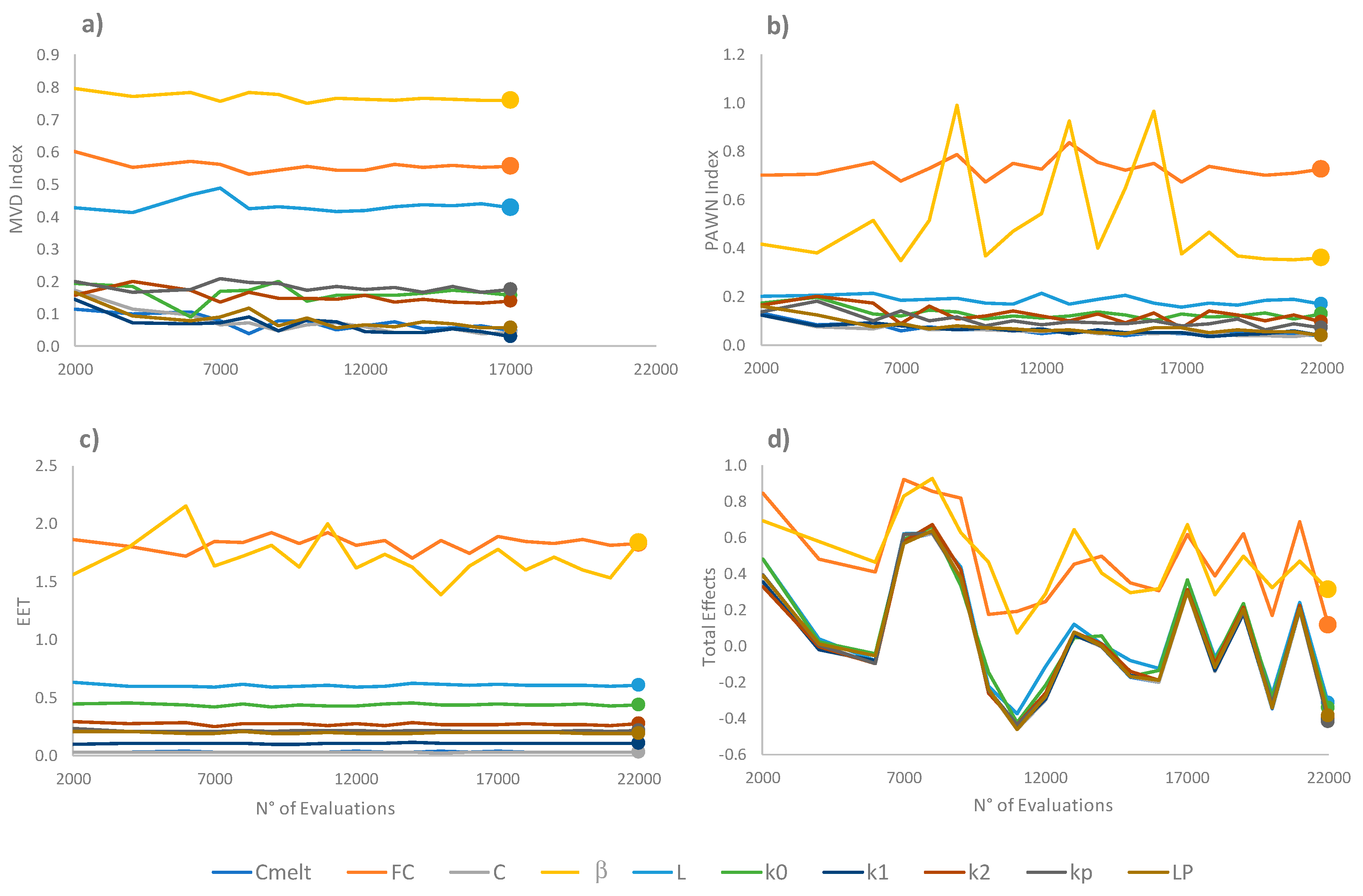
2.3. Convergence Analysis

To account for computational cost advantages of the proposed TVSA, a comparative convergence analysis was carried out for the application of the RSA, PAWN, Morris, and Sobol methods in a single 5-year window of the HVB model. To account for the costs, four variables were measured: (i) number of evaluations to reach convergence, (ii) the time consumed in performing the evaluations, (iii) the time needed for sensitivity index calculation, and (iv) the percentage of computer memory used during the sensitivity analysis. The SAFE TOOLBOX [4] with the HBV model (10 parameter version [27]) and the Allipén River basin were used for the analyses. A 5-year period (2001–2005) was analyzed with a daily time step configuration.

3. Application Example

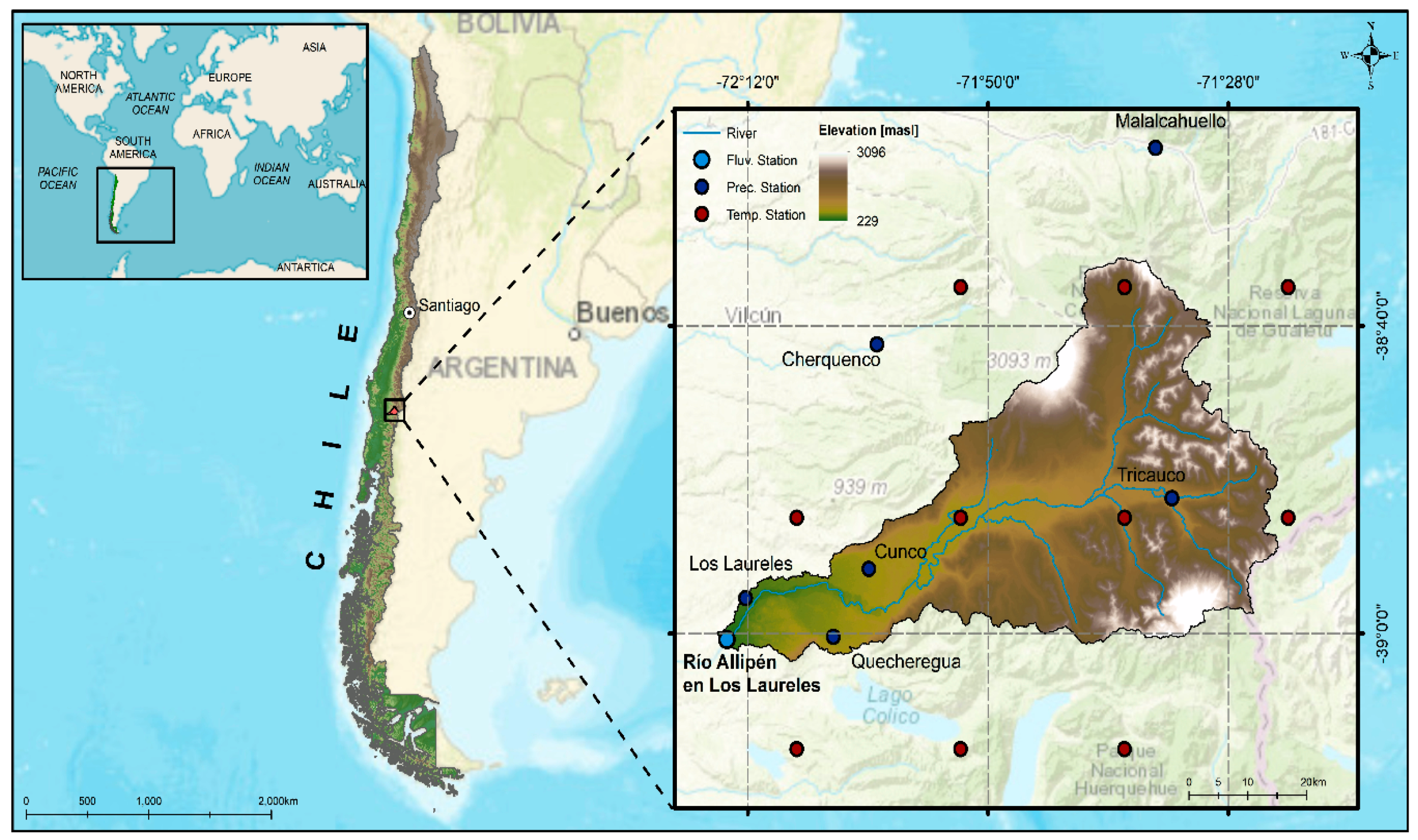
3.1. Study Area and Data

As an example of TVSA application, the script was implemented for the Allipén River watershed to the Allipén River at Los Laureles station (1652 km2), located in the south of Chile (Figure 2).
The Allipén River watershed is located on the western slope of the Andes Mountains. Annual precipitation is approximately 3000 mm and average monthly temperatures oscillate between −3 °C and 18 °C. The watershed receives mostly pluvial precipitation, with slight snow influence in the upper basin, presenting a mixed hydrological regime.
To implement the hydrological model of the watershed, the rainfall characterization was carried out using daily precipitation records from the 1951–2010 period from six rain gauge stations managed by the General Water Directorate (DGA) of Chile (see location in Figure 2).
Due to the absence of temperature records, 0.25°-resolution (~25 km) gridded data series published by the Princeton University Department of Civil and Environmental Engineering were used [40]. As a spatial data interpolation method, the inverse weighted distance method was used, and potential evapotranspiration was estimated using the Thornthwaite method [41].

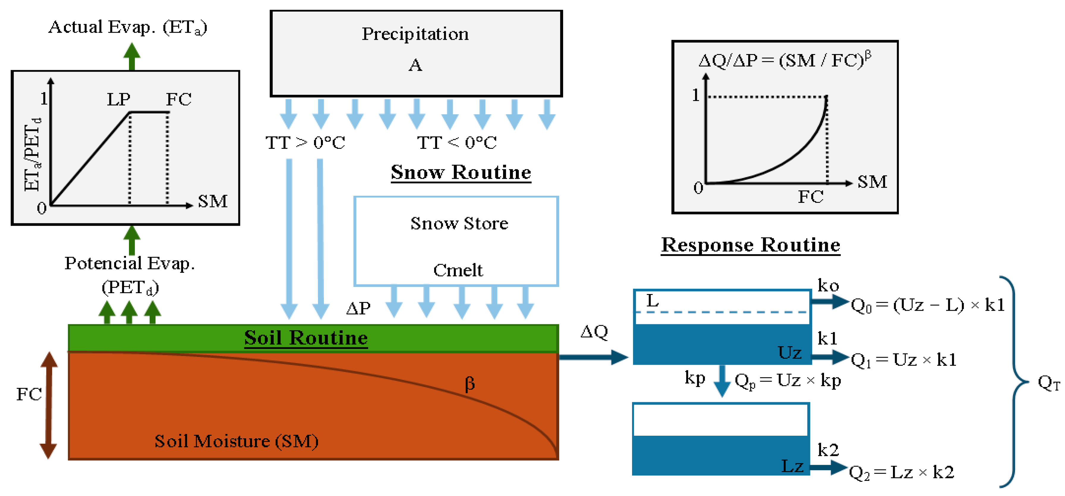
3.2. Description of the Model

To implement the TVSA and perform an assessment of temporal variability of environmental (hydrological in this study) processes, the HBV model was used. The HBV model is a lumped conceptual snow–rain water balance model. In this study, the simplified version developed by Aghakouchak and Habib [27] and based on Bergström [42] was used. The model simulates daily discharge based on daily precipitation, temperature, and potential evapotranspiration time series [42] and includes a snow routine, a soil routine, and a response routine (see conceptual diagram in Figure 3).
Precipitation is deemed to be snow or rain depending on the temperature on the corresponding day above or below a threshold temperature (TT). All precipitation is snow when the temperature is below TT, and all the snow contributes directly to the snow storage. If the actual temperature is greater than TT, there will be snowmelt. Snowmelt water is controlled by a degree-day factor (Cmelt), which determines the daily amount of melted snow depending on the difference between the actual and threshold temperatures. Subsequently, the sum of precipitation and snowmelt (ΔP) passes to the soil routine, which includes two modules. The first module calculates the actual evapotranspiration (ETa), which is equal to potential evapotranspiration (PETd) if the relationship between soil moisture (SM) and field capacity (FC) is above a threshold value for potential evapotranspiration (LP). However, for soil moisture values below LP, the actual evapotranspiration will be linearly reduced.
To calculate evapotranspiration, Bergström [42] introduced a routine that incorporates a correction factor (c) to obtain daily potential evapotranspiration (PETd) from daily mean air temperature and the long-term PET and monthly temperature averages.
Subsequently, the model calculates runoff (ΔQ), which depends on precipitation (ΔP), the actual water content of the soil (SM), the maximum soil moisture (FC), and an empirical coefficient (β), which determines the relative contribution of rain or snowmelt to runoff. Finally, the runoff response routine estimates the runoff at the watershed outlet. The system consists of two storage compartments, one above the other, which are directly connected to each other through a constant infiltration rate (Qp).
The upper deposit has two outlets (Q0 and Q1), whereas the lower deposit has one (Q2). When the water level in the upper deposit exceeds a threshold value (L), runoff is produced quickly in its upper part (Q0). The response of the other outlets is relatively slow. The streamflows are controlled by recession coefficients k0, k1, and k2, which represent the response functions of the upper and lower deposits. The constant infiltration rate (Qp) is controlled by a coefficient kp.
In order to ensure that the surface runoff process is quicker than the subsurface and groundwater runoff, the initial value of k0 must always be greater than k1. In addition, the response of the third outlet (groundwater runoff; Q2) must be slower than that of the second one (Q1); therefore, k2 must be lower than k1 [27]. For a better understanding of the model, see Bergström [42], Lindström et al. [43], and Seibert [44].
To adequately represent the spatial variability of precipitation and include the orographic effects in the study watershed, a precipitation adjustment factor (A) was considered in both models. This factor allows the model to obtain a long-term mass balance [45] and thereby correct the underestimation of precipitation resulting from the absence of records in the highest parts of each watershed. Table 1 presents a brief description of the parameters and initial ranges used, based on the studies of Aghakouchak and Habib [27] and Kollat et al. [46].

3.3. TVSA Implementation

To implement the TVSA, a Monte Carlo sampling of 10,000 points in the feasible space of each parameter, extracted from a uniform distribution, was carried out. According to Seibert and Vis [48], 1 year is sufficient to warm up the model. Therefore, the first year (1951) was not included in the subsequent analysis. Three TVSA were performed, at an annual time step in the 1952–2010 period, at a monthly time step in the 1990–1999 period and at a daily time step in the 1992–1994 period; windows of 5 years (n = 2), 3 months (n = 1), and 31 days (n = 15), respectively, were used.
The performed simulations were grouped as B and NB based on the Kling–Gupta Efficiency (KGE), with models presenting KGE values equal to or greater than 0.6 considered B, while models with KGE values less than 0.6 were considered NB.
To aid the understanding and analysis of the results and relate them to wet, dry, or normal years, the standardized precipitation index (SPI) [49] was calculated for a time scale of 12 months, as groundwater and catchment storage respond to precipitation alterations in the long term.
SPI helps to complement the assessments of temporal variability of environmental processes and permits to quantify the precipitation deficit for various time scales. According to the World Meteorological Organization (WMO) [49], it is effective for analyzing dry and wet periods. The index is simple to calculate, as the only parameter necessary for its calculation is precipitation. A period of at least 30 years of monthly values is recommended, but the optimum would be between 50 and 60 years, or more [49]. When choosing a time scale (i = 3, 6, 12, 24, or 48 months), for each month a value is determined with data from the i previous months. Each of the sets is fitted to a probability distribution, which is then transformed into a standardized normal distribution with a mean of 0 and variance of 1. Table 2 shows SPI values and their corresponding categories.
To classify years as normal, dry, and wet, the monthly SPI values were averaged per year, and the limits of the normal or near normal (NN) category (shown in Table 2) were considered, i.e., a year was considered wet when the averaged index was greater than 0.99, dry when the value was lower than −0.99, and normal when the value was between 0.99 and −0.99.

4. Results and Discussion

4.1. Computational Cost

Table 3 summarizes the computational costs of each sensitivity analysis method for the analyses of a 5-year window of the HVB model used in the Allipén River basin. All the sensitivity analyses were run on the same computer with 8 GB memory and 2.5 GHz CPU. The convergence of the sensitivity analysis was estimated based on the parameter stability after a certain number of evaluations. Figure 4 shows the convergence analysis performed for the RSA, PAWN, Sobol, and Morris methods in the Allipén River basin.
The results shown in Table 3 and Figure 4 indicate that the RSA requires fewer evaluations and less time than the remaining evaluated methods to obtain stable sensitivity indices. It also requires lower memory usage and consumes less time calculating the sensitivity index. The results are in line with the conclusions made by Sarrazin et al. [2].
As the TVSA depends directly on the number of evaluations and the computing cost of a sensitivity index used in a single window of evaluation, a TVSA based on RSA is simpler and cheaper in terms of computational cost. Because the proposed method is based on a simple RSA application, it results in a simpler TVSA that requires fewer evaluations and less computing cost than existing options.
Is important to point out that while running the HBV model for the Morris and Sobol methods, the computer used for this study ran out of memory before reaching full sensitivity index convergence.

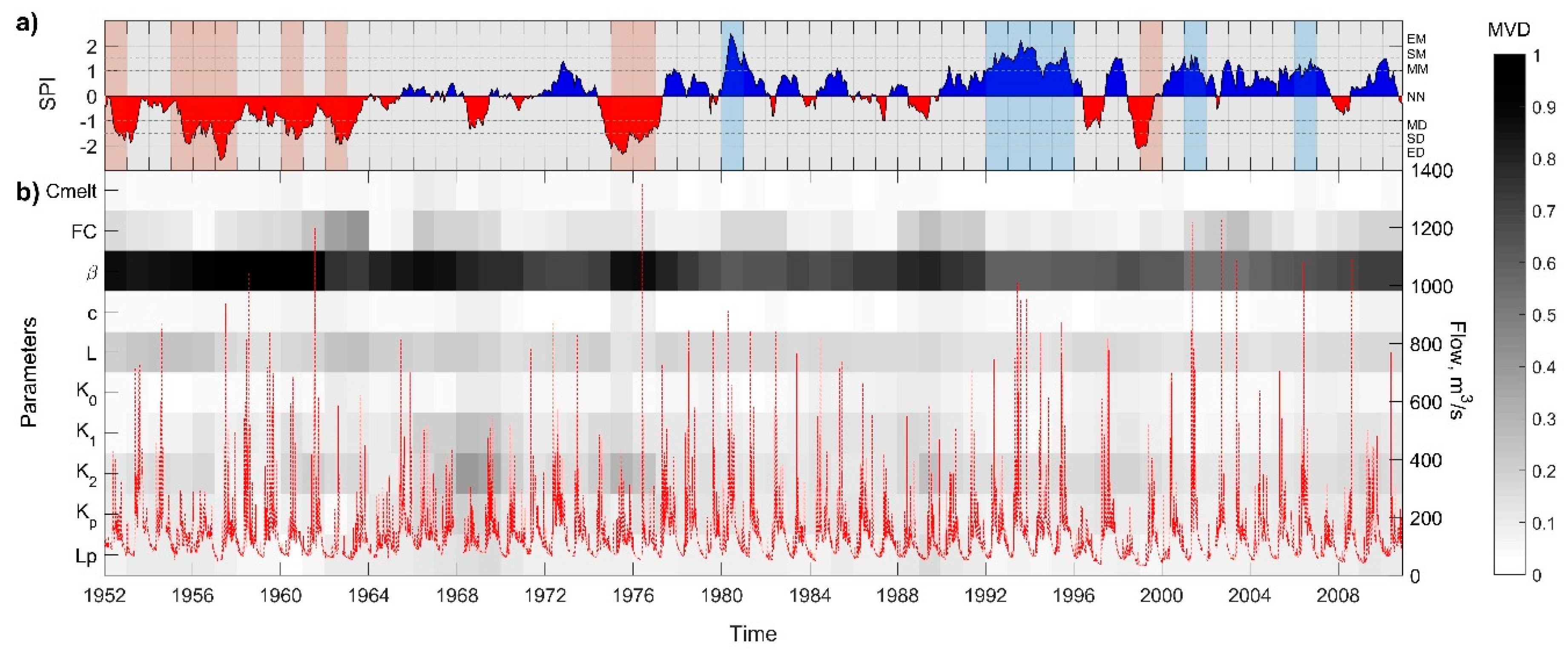
4.2. Temporal Variability of Hydrological Processes

Figure 5a shows the SPI calculated in the 1952–2010 period at a time scale of 12 months. According to the categories indicated in Table 1, the first 12 years are considered normal to dry years. Subsequently, a greater tendency toward normal to wet years is observed.
In Figure 5b the MVD index for a 5-year moving window (n = 2) in the 1952–2010 period is shown. It is observed that the main processes in the Allipén basin are those related to soil moisture, evapotranspiration, and groundwater. In addition, it is observed that the sensitivity of the model to β decreases/increases in wet/dry years, while the sensitivity to FC increases in wet years. It is also observed that the model is slightly more sensitive to K2 in dry years.
Figure 6a shows the monthly MVD index (n = 1) for the 1990–1999 period. During the winter months (July–September), the model is less sensitive to β and more sensitive to the FC and K1 parameters than for a 5-year moving window analysis. Meanwhile, during the summer months (January–March), the model is more sensitive to the K2, Kp, and Lp parameters and slightly sensitive to Cmelt.
Figure 6b shows the MVD index calculated for daily analysis with n = 15 (31-day window) for the 1992–1994 period. As in Figure 5a, in winter, the model is more sensitive to FC and K1 and less sensitive to β, whereas in summer, it is more sensitive to Lp, K2, Kp, and Cmelt.
The main watershed input is rainfall; therefore, due to high precipitation in the winter months (July–September), the highest streamflows are produced and the soil storage can reach a large part of its capacity. Thus, the processes present in the model that take on the greatest importance are soil moisture (FC) and quick response (K1 and Q1), which also indicate that β favors soil storage over runoff.
In the summer months (January–March), precipitation and streamflows decrease. During this period, streamflows depend mainly on groundwater contributions, which are represented in the model by the increase in sensitivity of the slow response (K2 and Q2) and percolation response (Kp and Qp). Temperatures in this period also increase; therefore, evapotranspiration (Lp and c) and snowmelt (Cmelt) take on more importance in the time of greatest precipitation. These results confirm the behavior identified through the model and proposed analysis. The results are consistent with the behavior of the watershed and findings of Abebe et al. [50], Zelelew and Alfredsen [51], and Pianosi and Wagener [20], where the model performance proves to be highly influenced by parameter β. Pianosi and Wagener [20] performed a TVSA based on PAWN for a 31-day moving window. They showed that the relative importance of model parameters over time can be distinguished. The TVSA shown in this study helps distinguish influential periods across data as well as for different aggregation times in the analysis (i.e., size of the time window). Therefore, it complements the existing TVSA options, allowing the same analyses as, e.g., those shown by Pianosi and Wagener [20], to be performed.

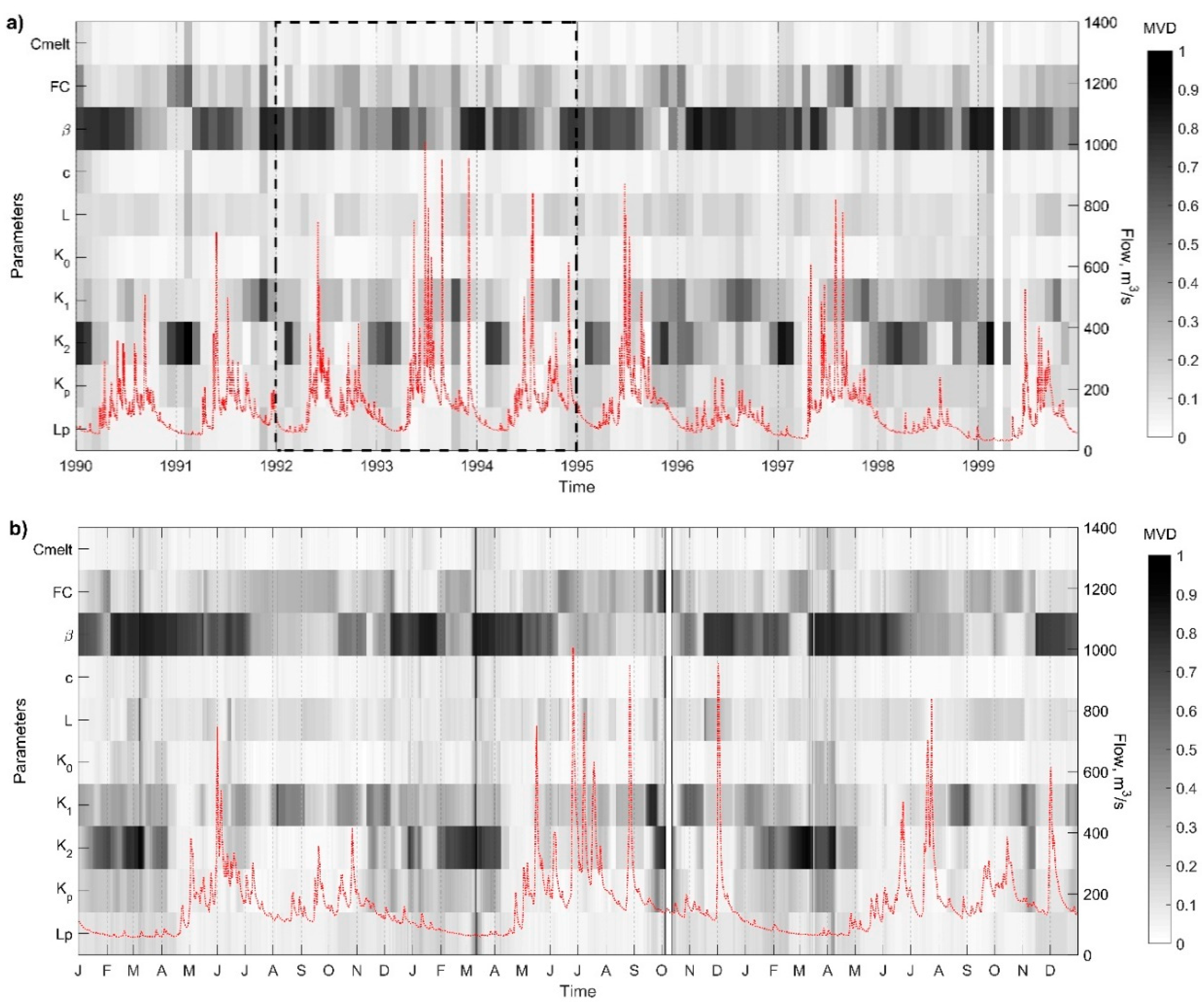
4.3. Size of the Window of Analysis

Although some differences between the 31-day and 3-month window sizes can be noticed, no significant differences among the most influential parameters are observed. However, when the window size for evaluation increases, the more aggregated processes take on greater importance and therefore, larger differences are noticed. For example, the larger the window for evaluation, the greater the importance of parameter β (see Figure 5a and Figure 6a,b). Regarding variability, the shorter the window size, the more the relative importance of parameter variability is noticed. These findings are probably related to the climatic variability of the study area where, e.g., climatic seasonality seems related to the hydrological model parameter variability observed in Figure 6a,b.
In both analyses (31-day and 3-month windows), the most relevant processes associated with wet and dry periods are detected. This indicates that, depending on the objective of the study, the choice of moving window and other assumptions can influence the estimation of sensitivity; therefore, the choice of time window size must be verified by performing the analysis for different moving window sizes, as is also described in Pianosi and Wagener [20] and Massman et al. [52].

5. Conclusions

In this study a simple function was developed that allows a TVSA with a low computational cost to be applied using the RSA method and MVD index. This function contributes to a better understanding of environmental processes and identification of their temporal variability. As an application example, the HBV model (10 parameters) was assessed using information from the Allipén River watershed, with the TVSA applied to 31-day, 3-month, and 5-year time windows. From the results, it is concluded that the most important processes in different periods and at different time scales can be detected and identified. In addition, it was observed that the MVD index allows the time sensitivity of a model with respect to its parameters to be detected independently, making it a suitable tool for assessment of aggregate models that include analysis of time series.
In the analyses, it can be observed that during the wet periods, the final streamflow is controlled by the field capacity (FC), whereas in the monthly and daily analyses, in recession periods the streamflow is controlled by groundwater (K2 and Kp) and snowmelt (Cmelt). Therefore, not only the choice of objective function, hydrological model, SA method, or study area but also the moving window size influences the estimation of sensibility indices in TVSA. To avoid errors in sensitivity estimation, a TVSA based on different moving window sizes is recommended.
The results shown in Table 3 and Figure 4 indicate that the RSA requires fewer evaluations and less time than the remaining evaluated methods to obtain stable sensitivity indices. It also requires lower memory usage and consumes less time calculating the sensitivity index. The results are in line with the conclusions made by Sarrazin et al. [2].
As the proposed method is based on a simple RSA application, it results in a simpler TVSA that requires fewer evaluations and less computing cost than existing options.

Supplementary Materials

The simple TVSA code used and presented in this paper is available online at https://www.mdpi.com/2073-4441/12/9/2463/s1.

Author Contributions

Conceptualization, TVSA method design, coding, analysis, methodology, application example, writing-original draft preparation, and visualization, Y.M. and E.M.; funding acquisition and supervision, E.M. All authors have read and agreed to the published version of the manuscript.

Funding

This research was funded by DINREG 03/2019 project.

Acknowledgments

The authors thank the Dirección General de Aguas (National Water Directorate) for providing the data used for the example of application of this study.

Conflicts of Interest

The authors declare no conflict of interest.

References

  1. Pianosi, F.; Beven, K.; Freer, J.; Hall, J.W.; Rougier, J.; Stephenson, D.B.; Wagener, T. Sensitivity analysis of environmental models: A systematic review with practical workflow. Environ. Model. Softw. 2016, 79, 214–232. [Google Scholar] [CrossRef]
  2. Sarrazin, F.; Pianosi, F.; Wagener, T. Global Sensitivity Analysis of environmental models: Convergence and validation. Environ. Model. Softw. 2016, 79, 135–152. [Google Scholar] [CrossRef] [Green Version]
  3. Norton, J. An introduction to sensitivity assessment of simulation models. Environ. Model. Softw. 2015, 69, 166–174. [Google Scholar] [CrossRef]
  4. Pianosi, F.; Sarrazin, F.; Wagener, T. A Matlab toolbox for Global Sensitivity Analysis. Environ. Model. Softw. 2015, 70, 80–85. [Google Scholar] [CrossRef] [Green Version]
  5. Devak, M.; Dhanya, C.T. Sensitivity analysis of hydrological models: Review and way forward. J. Water Clim. Chang. 2017, 8, 557–575. [Google Scholar] [CrossRef]
  6. Saltelli, A.; Ratto, M.; Andres, T.; Campolongo, F.; Cariboni, J.; Gatelli, D.; Saisana, M.; Tarantola, S. Global Sensitivity Analysis; Wiley: Chichester, UK, 2008. [Google Scholar]
  7. Borgonovo, E.; Plischke, E. Sensitivity analysis: A review of recent advances. Eur. J. Oper. Res. 2016, 248, 869–887. [Google Scholar] [CrossRef]
  8. Campolongo, F.; Saltelli, A.; Cariboni, J. From screening to quantitative sensitivity analysis. A unified approach. Comput. Phys. Commun. 2011, 182, 978–988. [Google Scholar] [CrossRef]
  9. Razavi, S.; Gupta, H.V. A new framework for comprehensive, robust, and efficient global sensitivity analysis: 2. Application. Water Resour. Res. 2016, 52, 440–455. [Google Scholar] [CrossRef]
  10. Razavi, S.; Gupta, H.V. A new framework for comprehensive, robust, and efficient global sensitivity analysis: 1. Theory. Water Resour. Res. 2016, 52, 423–439. [Google Scholar] [CrossRef] [Green Version]
  11. Khorashadi Zadeh, F.; Nossent, J.; Sarrazin, F.; Pianosi, F.; van Griensven, A.; Wagener, T.; Bauwens, W. Comparison of variance-based and moment-independent global sensitivity analysis approaches by application to the SWAT model. Environ. Model. Softw. 2017, 91, 210–222. [Google Scholar] [CrossRef] [Green Version]
  12. Cukier, R.I.; Fortuin, C.M.; Shuler, K.E.; Petschek, A.G.; Schaibly, J.H. Study of the sensitivity of coupled reaction systems to uncertainties in rate coefficients. I Theory. J. Chem. Phys. 1973, 59, 3873–3878. [Google Scholar] [CrossRef]
  13. Spear, R.C.; Hornberger, G.M. Eutrophication in peel inlet-II. Identification of critical uncertainties via generalized sensitivity analysis. Water Res. 1980, 14, 43–49. [Google Scholar] [CrossRef]
  14. Morris, M.D. Factorial sampling plans for preliminary computational experiments. Technometrics 1991, 33, 161–174. [Google Scholar] [CrossRef]
  15. Sobol, M.I. Sensitivity analysis for non-linear mathematical models. Math. Model. Comput. Exp. 1993, 1, 407–414. [Google Scholar]
  16. Pianosi, F.; Wagener, T. A simple and efficient method for global sensitivity analysis based oncumulative distribution functions. Environ. Model. Softw. 2015, 67, 1–11. [Google Scholar] [CrossRef] [Green Version]
  17. Razavi, S.; Sheikholeslami, R.; Gupta, H.V.; Haghnegahdar, A. VARS-TOOL: A toolbox for comprehensive, efficient, and robust sensitivity and uncertainty analysis. Environ. Model. Softw. 2019, 112, 95–107. [Google Scholar] [CrossRef]
  18. Wagener, T.; McIntyre, N.; Lees, M.J.; Wheater, H.S.; Gupta, H.V. Towards reduced uncertainty in conceptual rainfall-runoff modelling: Dynamic identifiability analysis. Hydrol. Process. 2003, 17, 455–476. [Google Scholar] [CrossRef]
  19. Guse, B.; Pfannerstill, M.; Strauch, M.; Reusser, D.E.; Lüdtke, S.; Volk, M.; Gupta, H.; Fohrer, N. On characterizing the temporal dominance patterns of model parameters and processes. Hydrol. Process. 2016, 30, 2255–2270. [Google Scholar] [CrossRef]
  20. Pianosi, F.; Wagener, T. Understanding the time-varying importance of different uncertainty sources in hydrological modelling using global sensitivity analysis. Hydrol. Process. 2016, 30, 3991–4003. [Google Scholar] [CrossRef] [Green Version]
  21. Ghasemizade, M.; Baroni, G.; Abbaspour, K.; Schirmer, M. Combined analysis of time-varying sensitivity and identifiability indices to diagnose the response of a complex environmental model. Environ. Model. Softw. 2017, 88, 22–34. [Google Scholar] [CrossRef] [Green Version]
  22. Zhao, Y.; Nan, Z.; Yu, W.; Zhang, L. Calibrating a hydrological model by stratifying frozen ground types and seasons in a cold alpine basin. Water 2019, 11, 985. [Google Scholar] [CrossRef] [Green Version]
  23. Wagener, T.; Kollat, J. Numerical and visual evaluation of hydrological and environmental models using the Monte Carlo analysis toolbox. Environ. Model. Softw. 2007, 22, 1021–1033. [Google Scholar] [CrossRef]
  24. Herman, J.D.; Kollat, J.B.; Reed, P.M.; Wagener, T. From maps to movies: High-resolution time-varying sensitivity analysis for spatially distributed watershed models. Hydrol. Earth Syst. Sci. 2013, 17, 5109–5125. [Google Scholar] [CrossRef] [Green Version]
  25. Herman, J.D.; Kollat, J.B.; Reed, P.M.; Wagener, T. Technical note: Method of Morris effectively reduces the computational demands of global sensitivity analysis for distributed watershed models. Hydrol. Earth Syst. Sci. 2013, 17, 2893–2903. [Google Scholar] [CrossRef] [Green Version]
  26. Herman, J.D.; Reed, P.M.; Wagener, T. Time-varying sensitivity analysis clarifies the effects of watershed model formulation on model behavior. Water Resour. Res. 2013, 49, 1400–1414. [Google Scholar] [CrossRef]
  27. Aghakouchak, A.; Habib, E. Application of a Conceptual Hydrologic Model in Teaching Hydrologic Processes. Int. J. Eng. Educ. 2010, 26, 963–973. [Google Scholar]
  28. Nash, J.E.; Sutcliffe, J.V. River flow forecasting through conceptual models part I—A discussion of principles. J. Hydrol. 1970, 10, 282–290. [Google Scholar] [CrossRef]
  29. Gupta, H.V.; Kling, H.; Yilmaz, K.K.; Martinez, G.F. Decomposition of the mean squared error and NSE performance criteria: Implications for improving hydrological modelling. J. Hydrol. 2009, 377, 80–91. [Google Scholar] [CrossRef] [Green Version]
  30. Medina, Y.; Muñoz, E. Analysis of the Relative Importance of Model Parameters in Watersheds with Different Hydrological Regimes. Water 2020, 12, 2376. [Google Scholar] [CrossRef]
  31. Pfannerstill, M.; Guse, B.; Fohrer, N. Smart low flow signature metrics for an improved overall performance evaluation of hydrological models. J. Hydrol. 2014, 510, 447–458. [Google Scholar] [CrossRef]
  32. Moriasi, D.N.; Arnold, J.G.; Van Liew, M.W.; Bingner, R.L.; Harmel, R.D.; Veith, T.L. Veith Model Evaluation Guidelines for Systematic Quantification of Accuracy in Watershed Simulations. Trans. ASABE 2007, 50, 885–900. [Google Scholar] [CrossRef]
  33. Parra, V.; Fuentes-Aguilera, P.; Muñoz, E. Identifying advantages and drawbacks of two hydrological models based on a sensitivity analysis: A study in two Chilean watersheds. Hydrol. Sci. J. 2018, 63, 1831–1843. [Google Scholar] [CrossRef]
  34. Wagener, T.; van Werkhoven, K.; Reed, P.; Tang, Y. Multiobjective sensitivity analysis to understand the information content in streamflow observations for distributed watershed modeling. Water Resour. Res. 2009, 45. [Google Scholar] [CrossRef] [Green Version]
  35. Singh, J.; Knapp, H.V.; Demissie, M. Hydrologic Modeling of the Iroquois River Watershed Using HSPF and SWAT ISWS CR 2004-08; Illinois State Water Survey: Champaign, IL, USA, 2004; Available online: http://hdl.handle.net/2142/94220 (accessed on 20 July 2019).
  36. Le Moine, N. Le Bassin Versant de Surface vu par le Souterrain: Une Voie D’amélioration des Performances et du Réalisme des Modèles Pluie-Débit? Ph.D. Thesis, Université Pierre et Marie Curie-Paris VI, Paris, France, 2008. [Google Scholar]
  37. Pushpalatha, R.; Perrin, C.; Le Moine, N.; Andréassian, V. A review of efficiency criteria suitable for evaluating low-flow simulations. J. Hydrol. 2012, 420–421, 171–182. [Google Scholar] [CrossRef]
  38. Pechlivanidis, I.G.; Jackson, B.; McMillan, H.; Gupta, H. Use of an entropy-based metric in multiobjective calibration to improve model performance. Water Resour. Res. 2014, 50, 8066–8083. [Google Scholar] [CrossRef]
  39. Patil, S.D.; Stieglitz, M. Comparing spatial and temporal transferability of hydrological model parameters. J. Hydrol. 2015, 525, 409–417. [Google Scholar] [CrossRef] [Green Version]
  40. Sheffield, J.; Goteti, G.; Wood, E.F. Development of a 50-year high-resolution global dataset of meteorological forcings for land surface modeling. J. Clim. 2006, 19, 3088–3111. [Google Scholar] [CrossRef] [Green Version]
  41. Thornthwaite, C.W. An Approach toward a Rational Classification of Climate. Geogr. Rev. 1948, 38, 55. [Google Scholar] [CrossRef]
  42. Bergström, S. The HBV Model—Its Structure and Applications; SMHI RH No. 4; SMHI: Norrköping, Sweden, 1992. [Google Scholar]
  43. Lindström, G.; Johansson, B.; Persson, M.; Gardelin, M.; Bergström, S. Development and test of the distributed HBV-96 hydrological model. J. Hydrol. 1997, 201, 272–288. [Google Scholar] [CrossRef]
  44. Seibert, J. Multi-criteria calibration of a conceptual runoff model using a genetic algorithm. Hydrol. Earth Syst. Sci. 2000, 4, 215–224. [Google Scholar] [CrossRef] [Green Version]
  45. Muñoz, E.; Rivera, D.; Vergara, F.; Tume, P.; Arumí, J.L. Identifiability analysis: Towards constrained equifinality and reduced uncertainty in a conceptual model. Hydrol. Sci. J. 2014, 59, 1690–1703. [Google Scholar] [CrossRef]
  46. Kollat, J.B.; Reed, P.M.; Wagener, T. When are multiobjective calibration trade-offs in hydrologic models meaningful? Water Resour. Res. 2012, 48, W3520. [Google Scholar] [CrossRef]
  47. Medina, Y.; Muñoz, E. Estimation of Annual Maximum and Minimum Flow Trends in a Data-Scarce Basin. Case Study of the Allipén River Watershed, Chile. Water 2020, 12, 162. [Google Scholar] [CrossRef] [Green Version]
  48. Seibert, J.; Vis, M.J.P. Teaching hydrological modeling with a user-friendly catchment-runoff-model software package. Hydrol. Earth Syst. Sci. 2012, 16, 3315–3325. [Google Scholar] [CrossRef] [Green Version]
  49. World Meteorological Organization. Standardized Precipitation Index User Guide. Available online: https://public.wmo.int/en/resources/library/standardized-precipitation-index-user-guide (accessed on 24 June 2020).
  50. Abebe, N.A.; Ogden, F.L.; Pradhan, N.R. Sensitivity and uncertainty analysis of the conceptual HBV rainfall-runoff model: Implications for parameter estimation. J. Hydrol. 2010, 389, 301–310. [Google Scholar] [CrossRef]
  51. Zelelew, M.B.; Alfredsen, K. Sensitivity-guided evaluation of the HBV hydrological model parameterization. J. Hydroinform. 2013, 15, 967–990. [Google Scholar] [CrossRef]
  52. Massmann, C.; Wagener, T.; Holzmann, H. A new approach to visualizing time-varying sensitivity indices for environmental model diagnostics across evaluation time-scales. Environ. Model. Softw. 2014, 51, 190–194. [Google Scholar] [CrossRef]
Figure 1. Code flow diagram. (a) Input window. (b) Objective function values. (c) Cumulative distribution functions of B and NB groups. (d) Graph of the MVD index at each window.
Water 12 02463 g001
Figure 2. Map of the Allipén River watershed, Chile, and locations of the measurement stations.
Water 12 02463 g002
Figure 3. Conceptual diagram of the Hydrologiska Byråns Vattenbalansavdelning (HBV) model [47].
Water 12 02463 g003
Figure 4. Convergence analysis performed for the (a) Regional Sensitivity Analysis (RSA), (b) PAWN, (c) Morris, and (d) Sobol methods. Lines indicate the sensitivity index related to each model parameter as a function of number of evaluations.
Water 12 02463 g004
Figure 5. (a) Standardized precipitation index (SPI) calculated for the 1952–2010 period. The left vertical axis shows the SPI values and the horizontal axis, time in years. The right vertical axis indicates the categories. The orange areas correspond to dry years, blue to wet years, and gray to normal years. (b) Maximum vertical distance (MVD) index for each year (5-year window). The left vertical axis shows the parameters, the horizontal axis, shows the time in years, and the right vertical axis shows the streamflow in m3/s as a reference. The dotted red line is the daily mean streamflow series. The MVD values are seen in grayscale.
Water 12 02463 g005
Figure 6. MVD calculated in windows of (a) 3 months (1990–1999) and (b) 31 days (1992–1994). The left vertical axis shows the parameters, the horizontal axis shows the time, and the right vertical axis shows the streamflow in m3/s. The dotted red line is the daily mean streamflow series (1990–1999). The MVD values are seen in grayscale. The white areas indicate that the index cannot be calculated.
Water 12 02463 g006
Table 1. Model parameters and initial ranges used for the analysis.
ParameterDescriptionRange
Mass balance
APrecipitation modification parameter0.8–2.5
Snow Module
TT (°C)Threshold temperature that indicates the initiation of snowmelt (normally, 0 °C)0
Cmelt ( mm ° C 1 day 1 ) Fraction of snow that melts above the threshold temperature (TT) from the beginning of snowmelt.0.5–7
Moisture module
FC (mm)Field capacity (storage in the soil layer)0–2000
β Empirical coefficient that represents the soil moisture variation in the area0–7
LPFraction of field capacity to calculate the permanent wilting point (PWP = LP × FC)0.3–1
C ( ° C 1 )Correction factor for potential evapotranspiration0.01–0.3
Response module
L (mm)Threshold for quick runoff response0–100
k 0 ( day 1 )Quick response coefficient (upper reservoir)0.3–0.6
k 1 ( day 1 )Slow response coefficient (upper reservoir)0.1–0.2
k 2 ( day 1 )Lower reservoir response coefficient0.01–0.1
kp (   day 1 )Maximum flow coefficient for percolation0.01–0.1
Table 2. Standardized precipitation index (SPI) values and categories.
SPI ValuesCategory
2 and aboveExtremely wet (EM)
1.5 to 1.99Severely wet (SM)
1.0 to 1.49Moderately wet (MM)
−0.99 to 0.99Normal or near normal (NN)
−1.0 to −1.49Moderate drought (MD)
−1.5 to −1.99Severe drought (SD)
−2 and belowExtreme drought (ED)
Table 3. Number of evaluations and computing costs associated with performing a single sensitivity analysis using different methods.
MethodEvaluations to Reach ConvergenceTime of Model Evaluation (s)Time for SI Calculation and Objective Functions (s)Memory (%)
RSA10,0001225.5575
PAWN19,0002317.3698
Morris>22,000 *246Out of memory
Sobol (TE)>22,000 *246Out of memory
TE: total effects; * maximum number of evaluation capable to be performed under the current hardware device.

