Abstract
The number of global open-source hydrometeorological datasets and models is large and growing. However, with a constantly growing demand for services and tools from stakeholders, not only in the water sector, we still lack simple solutions, which are easy to use for nonexperts. The new R package incorporates the BROOK90 hydrologic model and global open-source datasets used for parameterization and forcing. The aim is to estimate the vertical water fluxes within the soil–water–plant system of a single site or of a small catchment (<100 km2). This includes data scarce regions where no hydrometeorological measurements or reliable site characteristics can be obtained. The end-user only needs to provide a location and the desired period. The package automatically downloads the necessary datasets for elevation (Amazon Web Service Terrain Tiles), land cover (Copernicus: Land Cover 100 m), soil characteristics (ISRIC: SoilGrids250), and meteorological forcing (Copernicus: ERA5 reanalysis). Subsequently these datasets are processed, specific hydrotopes are created, and BROOK90 is applied. In a last step, the output data of all desired variables on a daily scale as well as time-series plots are stored. A first daily and monthly validation based on five catchments within various climate zones shows a decent representation of soil moisture, evapotranspiration, and runoff components. A considerably better performance is achieved for a monthly scale.
1. Introduction
The range of global hydrological models and their applications is vast and growing. These models are covering almost every possible niche in stakeholder’s needs: from water/food security and management tools [1] to flood warning systems [2]. One of the major intentions, and indeed a noteworthy one, is to cover the globe by a hydrological model or a dataset that can give stakeholders even in data scarce regions the opportunity to analyze, plan, govern, and decide on the historical and recent hydrological data.
There are numerous studies available on the application of hydrological models for various locations on the globe, suggestions of global parameterizations and their performance [1,3,4,5,6,7,8,9,10,11]. However, all these models were parameterized by deploying local (i.e., regional, national) datasets of high quality and calibrated to observed discharge data before discussing their performance. On the other side, there are already a few global datasets with major components of the hydrological cycle (i.e., precipitation, evapotranspiration, soil water, runoff) available, which are regularly updated in operational mode (JRA-55 [12], MERRA2 [13], NCEP Climate Forecast System Version 2 (CFSv2) [14], ERA5 [15]). In this case, the resolution of the grid cells was approximately 50 km, which is mostly a tradeoff between the current computational capabilities and the complexity of global climatological models. Therefore, two limitations become obvious and open a potential gap or, more precisely, a challenge. Namely, of gaining highly resolved water cycle components at any location on the globe by an easy model setup and globally available parameterization and meteorological forcing datasets. This challenge was discussed already in 2011 [16] stating that hyper-resolution (i.e., <1 km2) of modeling the global land-surface hydrological processes is critical for scientific and practical needs (for the better understanding and predictability of surface–subsurface and land–atmosphere interactions, water quality and human impacts on the water cycle) but impossible at the moment within current modeling capabilities. Some of the models used in the aforementioned studies are already presented as framework solutions with data input and data processing. Even more, they partly consider model calibration, applications, and result assimilation. There are framework packages in Python [17] and R [18].
Yet, there is to our knowledge no automatic modeling framework “from A to Z” available currently, which incorporates automatic data assimilation, a deterministic hydrological model application, and result postprocessing for any desired location on the globe, and at the same time capable to run on a personal computer.
Recent developments in global datasets show an increase of resolution and quality of the data, which could be used for the parameterization of land cover and soil characteristics and as meteorological forcing of hydrological models. Keeping in mind, that “all models are wrong but some are useful” [19], it becomes a doable challenge to test whether such a framework could be developed in a simple and easy-to-use black-box (or nonexpert) version and still give adequate results for the governing components of the water balance on small spatial scales, starting from a few meters.
For this purpose, the lumped hydrologic model BROOK90 [20] was enabled to gain location related information of parameters and the meteorological input from the ERA 5 [15], the Global Land Cover [21], and the SoilGrids250m [22] datasets.
The main objectives of this study are:
- To broaden the BROOK90 community by expanding the scope of its application;
- To show the opportunities and limitations of the globally applicable modeling framework based on a lumped physical model and open-source input data;
- To simplify a hydrological framework emphasizing usability for nonexperts by full automation of the modeling process in a R package under the motto: “Just drop a catchment and receive a model output”;
- A contribution to the open-source hydrological science community by the release of the package code.
The research questions of the paper are stated as following:
- Is reasonable location-related model output achievable by deploying a noncalibrated lumped hydrological model based on global parameterization and forcing datasets?
- What are potential uncertainties and limitations of such a framework?
2. Description of the Framework
The description of Global BROOK90 is divided in three main parts, followed by technical remarks on the package. At first, an introduction to the original BROOK90 hydrological model itself is presented. Then, the main input open-source datasets used in the model parameterization are described. Finally, the core functions of the framework are introduced that unite the user input, data download and processing, model parameterization and run, and result postprocessing.
2.1. Short Introduction to the Original BROOK90 Model
BROOK90 [23] is a physical lumped hydrological model with a special focus on a detailed representation of vertical water fluxes within the soil–water–plant system at a single site.
Precipitation, maximum and minimum air temperature, solar radiation, vapor pressure, and wind speed on a daily time scale are the standard meteorological input variables (i.e., input of precipitation in higher temporal resolution is possible). Figure 1 shows the model flowchart. It illustrates how the model stores canopy-intercepted rain or snow, the snow storage on the ground, the water in the soil layers, and the groundwater. Net throughfall of precipitation, which was not intercepted by the vegetation, together with the snowmelt either infiltrates (into the soil matrix or into deeper layers by macropores) or concentrates directly to streamflow (overland or vertical macropore flow followed by downslope flow). Additionally, a delayed contribution to the streamflow from vertical or downslope soil drainage and groundwater storage is simulated. Soil water movement is described within several layers by saturated and unsaturated matrix flow and macropore flow using Richard’s equation. The parameterization of the soil allows for up to 25 layers (which number is technically possible to extend) and a detailed representation of matrix flow, e.g., depending on uptake by the roots driven through transpiration.
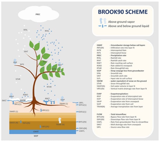
Figure 1.
Water fluxes and processes represented in BROOK90 [24].
Groundwater storage changes by gravity drainage from the deepest soil layer and seepage is modeled via a fixed fraction of groundwater outflow. The evapotranspiration process consists of five components: evaporation of intercepted snow/rain from the canopy, evaporation from snow/soil, and transpiration from a single layer canopy. The resistance framework is built on the Shuttleworth–Wallace approach and allows modeling dense canopies like a forest plantation in temperate climate, but also sparse, open canopies like savannas. For a detailed process description and calculation approaches used, please refer to the original documentation [20].
The main known limitations of BROOK90 [20] are the following: lateral water movement towards downslope areas is not recognized, the model has no implementation of channel routing, hillslope processes are neglected, plant phenology is missing, the vegetation layer is uniformly distributed, and soil frost is not taken into account. Moreover, as the model does not consider the inflow of soil and groundwater, it is not suitable for environments where the vegetation has access to shallow groundwater. Among the unquestionable benefits of BROOK90 are the assumption of the basic physical principles of mass and energy conservation, daily model output based on subdaily routines, a complex evapotranspiration scheme, and a good representation of soil moisture fluxes.
Overall, hydrologists recognize BROOK90 as a useful tool for studies of the water balance for small plots in mainly forested regions (i.e., from the most recent studies [25,26,27,28,29]). Therefore, it has been used in research, teaching, and water management, and also because of its ability to gain reasonable results even under changing climate conditions [20].
2.2. Input Open-Source Datasets
Three main datasets are incorporated in the framework of the package. These provide the necessary meteorological, vegetation, and soil input data for the BROOK90 model. A short overview of the datasets is presented in Table 1.

Table 1.
Summary of the input datasets.
The ERA5 global climate reanalysis dataset from Copernicus and European Centre for Medium-Range Weather Forecasts [15] (1979–present, hourly resolution) is used as meteorological forcing of the BROOK90 model in the package. The ERA5 dataset is based on a combination of a global physical model of the atmosphere and observations from across the world using data assimilation principles. This means that the current timestamp of the model run combined with observations is used to derive the next model timestamp. The dataset is accessed via the MARS (Meteorological Archival and Retrieval System) request builder and the “ecwmfr” R package [30]. The following variables are retrieved: 2 m air temperature [K], surface net solar radiation [J m−2], precipitation [m], and wind speed in two dimensions [m s−1]. The original model resolution is 0.28125°. This is equivalent to approximately 31 km. It is possible to download ERA5 data on a custom grid and horizontal resolution; however, the data are resampled from the original resolution. The default interpolation method for continuous parameters is bilinear and does not improve the accuracy of the data [31]. For the convenience of further data processing, a 0.1° × 0.1° grid size and an “ncdf” (network Common Data Form) output file format is used. The biggest limitations of the dataset are the server restrictions: data retrieval per request is limited to a maximum of 120,000 items (~13 years for five variables) and download speed is strongly affected by the query length of other users’ requests. Developers and researchers claim a high quality of the data with regard to a global coverage and the temporal resolution [32,33,34,35,36]. The uncertainty of the dataset can be estimated by the analysis of 10 reanalysis ensemble members, while in the package presented the mean reanalysis output is used. However, it is possible to implement and deploy an ensemble of meteorological forcing, yet with a two times coarser spatial resolution.
The SoilGrids250 product [22] provides global information on standard soil properties with a spatial resolution of 250 m. The product is based on machine learning algorithms (namely, random forest, gradient boosting, and multinomial logistic regression) using a large database of worldwide available soil profiles as predictors and remotely sensed measurements as covariates. The following information on soil properties from SoilGrids250 is used:
- Soil texture classes (USDA system, 12 classes: sand, loamy sand, sandy loam, loam, sandy clay loam, silt loam, silt, silty clay loam, clay loam, sandy clay, silty clay, clay);
- Volumetric fracture of coarse fragments [%] at seven standard layers (0, 5, 15, 30, 60, 100, and 200 cm);
- Soil depth to the bedrock [cm] (R horizon).
Data are retrieved as “tiff” (Tagged Image File Format) rasters via an API request for the specific coordinate extent from a TU Dresden Geoserver [37]. A global 10-fold cross-validation performed by the developers showed an average prediction error for key soil properties (based on R2) in the range of 54–79%. The predictability is more limited for the variable “depth to the bedrock” and increases for the soil classes. A comparison between various existing soil datasets in the context of model applicability concluded that SoilGrids250 is the current state-of-the-art soil dataset [38]. Some hydrologists have already applied it in their studies [39,40,41,42,43].
The second version of the Land Cover 100 m dataset released in 2019 and distributed by the Copernicus Global Land Service [21,44] represents the 2015 epoch (three-year period giving reference year +/− one year). It covers 23 discrete classes: 12 forest types (evergreen/deciduous, needleleaf/broadleaf, closed/opened, mixed, and unknown), shrubs, herbaceous vegetation, herbaceous wetlands, moss and lichen, bare/sparse vegetation, cropland, urban/built-up areas, snow and ice, permanent water, ocean, and no data. The dataset was obtained using PROBA-V satellite time-series, global training data generated with Geo-Wiki and Google/Bing imagery, and biome-cluster classification algorithms. This algorithm was chosen in order to adapt the algorithm to subcontinental and continental patterns [45]. The original tiles (20° × 20°) [46] were aggregated in one raster and can be accessed at TU Dresden Geoserver by using the location coordinates [37]. In accordance to the validation reports [47,48] the overall classification accuracy is approximately 80% (forest subclasses excluded). The highest accuracy was achieved for forest, bare/sparse vegetation, snow/ice, and permanent water bodies (>85%). The lowest performance was observed for shrubs, herbaceous wetland, and moss/lichen (<65%). The global accuracy yields to 75% with consideration of the forest types in the validation. Currently, the Global Land Cover dataset has global spatial coverage, and the finest spatial resolution and largest number of vegetation types in comparison with all other known alternatives (i.e., ESACCI [49], MCD12Q1 [50], GLC2000 [51], GLOBELAND30 [52]).
Additionally, a digital elevation model (DEM) is required for the calculation of a few orographic characteristics of the catchment, like mean slope and aspect. These are required for the estimation of solar radiation and subsequently evaporation and snowmelt. The DEM is accessed by the using the “elevatr” R package [53], which gives access to various DEMs available in Amazon Web Service Terrain Tiles. The service automatically chooses the dataset with the best resolution for the desired territory: 3DEP [54], ArcticDEM [55], CDEM [56], open data portals of UK [57] and Austria [58], ETOPO1 [59], EUDEM [60], GMTED [61], INEGI [62], Kartverket [63], LINZ [64], SRTM30 [65]. In general, the resolution varies from 3 m to 2.5 km.
Figure 2 shows an overview on all datasets collected by the “Global BROOK902” package needed for a simulation of an exemplary catchment of Alto river located on Corsica island, France (104 km2).
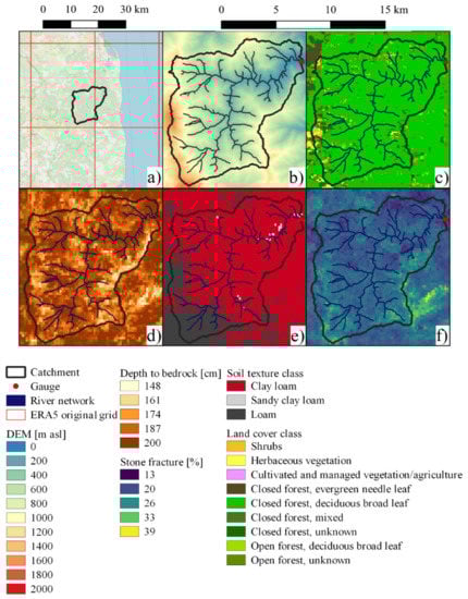
Figure 2.
Outlook on the input datasets (WGS-84 Pseudo-Mercator projection) for Alto river–Taglio–Isolaccio (42.44° N 9.47° E, Corsica, France): ERA5 [15] grid tiles with OpenStreetMap as background [66] (a); digital elevation model based on SRTM30 [65] (b); Global Land Cover [21] classes (c); SoilGrids250 [22]—depth to bedrock (d), soil texture classes (7th layer) (e), and soil coarse fragment fracture (7th layer) (f).
2.3. Core Functions, Framework, and Parameterization
The package workflow consists of five milestones (Figure 3): input from user (1), data download (2) and processing (3), BROOK90 application (4), results postprocessing and storage (5). Therefore, four core files (data_downloader, data_processing, model_hydrotope, and brook_framework) and the following main functions are implemented:
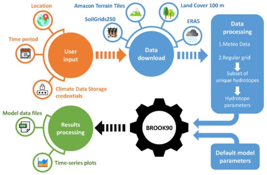
Figure 3.
Scheme of package framework. (Icons made by Freepik from www.flaticon.com).
- brook90.framework. This is the core function of the package. It has only one call function that is visible to the user. It requires the following minimum input information: the path to the catchment shape file (“shp”), the Climate Data Store (CDS) credentials, and the modeling time interval. Incorporating all the functions mentioned below, it creates the necessary (sub) folders in the workspace (if not provided, then it is the location folder of the shp file). It saves the downloaded initial data (land cover, soil and meteorological data, DEM) and runs the BROOK90 routine, and then postprocessing is performed. Finally, it saves the model output results (“csv” files and “png” time-series plots for each variable, “csv” file with hydrotopes and their characteristics).
- download.landcover/download.soil/download.dem/download.meteo. These functions download data required for the model using the data location of the catchment shape file and output folders for each data type (for meteorological data additionally CDS credentials and desired time interval). They create and send API requests and then retrieve and store files. Specifically, these are “tiff” files of the catchment’s land cover classification and soil texture classification, stone fraction, depth to the bedrock, and DEM with a ~1 km buffer zone, and the “ncdf4” files for temperature, precipitation, solar radiation, and wind speed.
- data.processing. This function at first constructs a regular grid over the catchment and creates a subset of hydrotopes. Secondly, it prepares and returns the input for the BROOK90: hydrotope parameters and the processed meteorological data.
- brook90.run.subcatchment. The function runs BROOK90 (R version [24]) for a specific unique hydrotope by merging the default BROOK90 parameters with the ones related to the desired hydrotope and executing the model routine. It returns daily time-series of the requested variables.
The specifications of data and initials which have to be provided by the end-user are:
- A catchment (or site) shapefile in WGS-84 coordinates. Currently, only polygons with continuous borders without gaps inside or self-interception are permitted.
- A time interval for the modeling. This interval is limited by the meteorological input dataset: from 2 January 1979 to the current date minus a week.
- The credentials for the meteorological data download. These consist of the username and key to the Copernicus Climate Data Store (CDS). It can be obtained after registration on the Copernicus website. Before running the framework for the first time, the terms of use of Copernicus products have to be accepted.
- Optional input information:
- ◦
- The model output folder (default is the same folder of the catchment “shp” file);
- ◦
- The list of output variables (default outputs are soil water content, total runoff, evapotranspiration, precipitation);
- ◦
- The number of days to cut from the output (model “warm-up” period, default is 30 days);
- ◦
- The method of raw ERA5 data averaging (default is weighted mean).
The first step in the package framework when the user is calling the main brook90.framework function consists of a data download. For the extent of the catchment, land cover, soil, and meteorological data are downloaded. They are stored in the corresponding folders created in the model directory. While soil data are retrieved via images, land cover data and the DEM are provided in tiles and need much more time for downloading, unpacking, and clipping. The ERA5 download is implemented as a process that performs multiple requests to overcome the limitation of maximum items per request (~13.7 years of hourly data for one variable). For instance, to cover the period of 1979–2020, 15 requests are needed (i.e., three time divisions for five meteorological variables).
The preparation of the meteorological data starts with an averaging of the downloaded data for the catchment extent. Three methods are available. The first is to take the nearest to the catchment’s geometric mass center grid. The second calculates a mean value out of all downloaded cells, and the third derives an area-weighted mean by the interception of the catchment’s borders with the regular ERA5 grid. Afterwards, daily minimum and maximum temperature are derived from the hourly data. Furthermore, the calculation of the mean wind speed and mean daily actual vapor pressure (after Bougeault [67]), as well as the upscaling of hourly wind speed and solar radiation data to a daily resolution are performed. Additionally, the data timing is corrected according to the respective time zone and a time shift of −1 h is applied for precipitation [31].
The subset of unique hydrotopes plays a crucial role in the package. A hydrotope is defined by a unique combination of land cover and soil texture type, stone fraction, and depth to bedrock located within the catchment. Since land cover and soil data have different resolutions, a regular grid of 50 × 50 m is constructed over the catchment. The length and the width of a grid cell are adjusted according to the length and width of the longitudinal and the latitudinal degree at the catchment location. However, while land cover and soil texture are coded for each layer with fixed integer indexes, soil stone fracture is presented in percent and soil depth to the bedrock in cm. Thus, to reduce the possible number of unique combinations, the following algorithm is proposed. At first, the depth to the bedrock is reclassified by rounding to 10 cm steps. Secondly, hydrotopes are subset by means of unique land cover, soil texture, and reclassified depth to the bedrock. Finally, all values of the soil stone fraction for each specific layer, which corresponds to a specific subset of unique combination of land cover, soil texture, and depth to bedrock, are averaged to one value per layer and assigned to a specific hydrotope. Additionally, the frequency of the hydrotope occurrence within a catchment is stored for the further processing.
The vegetation of a hydrotope is parameterized using land cover data. For each land cover type, except for “permanent water bodies” and for “open sea”, a unique parameter set is defined. Therefore, the initial recommendations from the BROOK90 documentation [20] are followed. They are adapted and enlarged by the additional studies of [68,69,70,71,72,73]. The following vegetation parameters are recognized:
- relative height (fraction of maximum annual plant height for each vegetation period),
- relative leaf area index (fraction of maximum annual leaf area index for each vegetation period),
- soil and snow albedo,
- reduction factor for snow evaporation in tall canopies,
- ground surface roughness,
- maximum annual plant height,
- maximum annual leaf area index,
- maximum length of fine roots per unit ground area,
- xylem fraction of plant resistance,
- maximum leaf conductance,
- average leaf width,
- extinction coefficient for photosynthetically active radiation in the canopy,
- relative root density (per unit stone-free volume) of fine or absorbing roots for given layer,
- fraction of impermeable soil.
The soil hydraulic characteristics for a hydrotope are parameterized using soil texture classes following the recommendations from the model documentation [20]. These classes were derived by field experiments (remark: silt-loam parameters were assigned for the silt soil type, since it is missing in original documentation). The following parameters of soil are used to characterize the soil column in general and each of the layers specifically:
- total number of soil layers in the column,
- thickness of each layer,
- volumetric stone (coarse fragment) fracture of each layer,
- soil matrix potential at field capacity of each layer,
- volumetric soil water content at field capacity and full saturation of each layer,
- exponent of matrix potential–wetness relationship of each layer,
- hydraulic conductivity at field capacity of each layer,
- soil wetness at the dry end of the near-saturation range of each layer.
Initially, the package creates a standard 200 cm profile with characteristics for each of the layers. However, if the value of the depth to the bedrock is less than 200 cm, the soil column is cut from the bottom to an appropriate depth by means of reduction of layer thickness or the whole layer(s) with its parameters.
The derived parameters of each hydrotope together with meteorological forcing and the environment with the default model parameters are then passed to BROOK90. The model is sequentially executed for each hydrotope. Originally implemented in FORTRAN [23], BROOK90 was translated into the R language in 2018 [24] and the latter code is used as a model routine.
Finally, the outcome of each hydrotope model run for the requested list of variables is allocated in a list of data frames. The daily area-weighted averages are calculated according to the hydrotope occurrence frequency. The results are stored in the model output folder together with standardized time-series plots.
While running the package, all main steps as well as time benchmarks are printed as status messages on the RStudio console to trace the execution of the major routines of the framework’s application.
2.4. Technical Remarks
The presented package was developed in R language [74] (version 3.5.2) and operates as an R project in an RStudio [75] environment (version 1.1.383 or higher). Internet access and ~3 GB of free hard drive space are necessary. The hard drive space is required to download and install the package and to store the model input data and results afterwards. The package is currently stored and will be updated in a Github repository [76]. It can be accessed as an RStudio project and installed using the standard project “Build” tool. Additionally, the “pacman” [77] package needs to be installed. This package will take care of the automatic download and installation of the additional R packages required to run “Global BROOK90”. These are: “raster” [78], “elevatr” [53], “rgdal” [79], “sp” [80], “ecwmfr” [30], “keyring” [81], “lubridate” [82], “rgeos” [83], “stringr” [84], “plyr” [85], “data.table” [86], “ncdf4” [87], “lutz” [88], “ggplot2” [89].
The framework occupies one CPU core and was tested on two different machines: a personal computer (CPU/RAM: 3.4 GHz/15 GB) and a laptop (CPU/RAM: 1.9 GHz/4 GB). The normalized average computational time was estimated by approximately 13 s/23 s for one hydrotope and 1 year with an hourly simulation step. The download of elevation, land cover, and soil data depends fully on the speed of the internet connection (estimated as 10 to 20 min). Apart from that, the download situation for the ERA5 retrieval is different. It depends mainly on the CDS server load and the amount of requested data (per request and per day) and could last for about 9 to 12 h for a complete 1979–2020 period. But once the data are already downloaded, in case of a new model run the data download will be skipped.
3. Results and Discussion
The performance and first validation of the results are discussed on the basis of five catchments from Iceland, USA, Canada, Germany, and Indonesia. They were selected for two reasons. First, they are located within different climate zones, and second, they have various relief, land cover, and soil texture (Figure 4, Table 2). To evaluate the performance of the package, two strategies were applied. The first one is to compare the runoff component to the observed discharge data provided by the Global Runoff Data Centre [90]. For the chosen catchments, the following observed time-series are used, respectively: 1979–2018, 1979–2006, 1979–2017, 1979–2016, 1979–2009. The second strategy is to compare the soil water content, evapotranspiration, and runoff to the similar variables available within the ERA5 reanalysis.
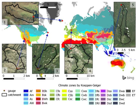
Figure 4.
Outlook on the chosen catchments (WGS-84 Pseudo-Mercator projection) with Koeppen–Geiger world climate zones [91] and Bing images [92] as background. Numbers near the catchments refer to Table 2.
Table 2.
Characteristics of chosen catchments.
Figure 5 and Figure 6 depict the results of the model runs for the major water balance components: soil moisture, evapotranspiration, and runoff on monthly and on daily scales. The soil moisture time-series show that three out of five catchments have clear annual cycles. Minimum–maximum range analysis for all hydrotopes reveals large deviations of some hydrotopes from the catchment weighted mean. Sometimes, this deviation is up to 100%. The evapotranspiration, on the other hand, has a larger interannual variance. The chosen catchments show annual cycles with lowest values for bare/sparse vegetation and highest for broadleaf forests. The runoff plots together with the knowledge of the climate zone allow for distinguishing between the main flood formation factors; i.e., rain seasons for catchments 2 (arid) and 5 (tropics), while others are of a mixed genesis (snowmelt and rainy season). Additionally, big variations in peak runoff between individual hydrotopes can be seen. The highest values for all three variables, with no surprises, were observed in the tropics. However, it should be noted that the absolute values of soil moisture could be severely affected by the uncertainty in the soil column depth estimation (see Section 2.2).
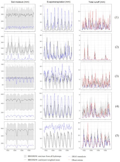
Figure 5.
Monthly time-series of modeled (weighted mean and maximum/minimum range from all hydrotopes) soil water content, evapotranspiration, and runoff (overlapped with observation line) for the chosen catchments (numbers on the right side refer to Table 2).
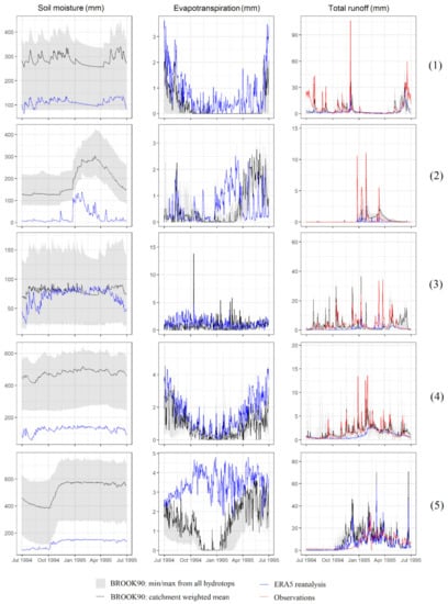
Figure 6.
Daily time-series of modeled (weighted mean and maximum/minimum range from all hydrotopes) soil water content, evapotranspiration, and runoff (overlapped with observation line) for the chosen catchments (numbers on the right side refer to Table 2).
In general, the similar global soil parameterization scheme used in the package appears in the land surface model of ERA5. Soil moisture (the original variable is volumetric soil water content) in ERA5 was also derived according to Darcy’s law and with standard soil profiles (four layers). Constant hydraulic characteristics were assigned based on seven different soil textures of the root zone from the FAO/UNESCO Digital Soil Map of the World [93] (~10 km resolution). The seasonality within both monthly and daily interannual cycles obviously behave similarly (except for catchment 3), while large absolute differences could be explained by different soil profile depths used in BROOK90 and ERA5.
While evaporation processes from surfaces in both models have an equivalent level of specification, transpiration in BROOK90 has a more physically detailed representation. The HTESSEL land surface model [94] for the ERA5 uses 1 × 1 km Global Land Cover Characteristics [95] to parameterize 16 vegetation types with five globally fixed parameters (seasonality is represented with leaf area index). The “Global BROOK90” package, on the other hand, has a set of 13 parameters for 18 vegetation types with a 10 times higher dataset resolution.
Focusing on the five catchments, ERA5 gives higher evapotranspiration rates and earlier annual peaks on the monthly scale, especially in winter months. On daily basis, BROOK90 tends to have slightly smaller day-to-day variation. Completely different results for catchment number 5 indicate various representation of the tropical forest in two parameterization schemes, as well as a coarser resolution of ERA5 itself.
The total runoff component from both BROOK90 and HTESSEL is the sum of surface (excess of infiltrability from net throughfall or snowmelt) and subsurface (lateral/downslope and bypass flow in BROOK90 and simple resulting vertical drainage in HTESSEL) components [20,96]. Despite that the models are driven by the same precipitation forcing, the runoff response is different. A general underestimation of the water volume in ERA5 for catchments 1–4 leads to a shortage of low flow conditions and flood peaks on both daily and monthly scales. Runoff from “Global BROOK90” possesses a much better agreement with the observations regarding annual cycles and daily variability, although it can potentially overestimate low flow conditions and is unable to capture the magnitude of flood peaks.
For the quantitative analysis of the package performance, conventional Nash-Sutcliffe Efficiency (NSE) [97] and Kling-Gupta Efficiency (KGE) [98] skill-scores were calculated for the two temporal scales (Figure 7). It can be seen that the performance of simulated weighted mean runoff on a daily scale according to both NSE (0.36, 0.07, 0.16, 0.28, −0.56) and KGE (0.38, 0.15, 0.44, 0.42, 0.31) was noticeably lower than for the monthly averages (NSE: 0.26, 0.09, 0.02, 0.33, 0.13; KGE: 0.43, 0.53, 0.38, 0.47, 0.54). The addition of NSE and KGE values for all hydrotopes illustrates that for all tested catchments at least one hydrotope performed better than the model weighted mean. Thus, some of the hydrotopes raised skill-score values up to 0.8. This comparison is also valid since technically BROOK90 as a lumped model treats all unique hydrotopes as independent area-dimensionless pseudo-catchments with the same meteorological forcing. Furthermore, it was found that the accuracy of ERA5 runoff is much lower (except only daily NSE for catchment 5) in comparison to the BROOK90 results. Nonetheless, these performance results should be treated with caution, since BROOK90 is actually a lumped water balance model and the model used in ERA5 cannot account for flow accumulation and routing between hydrotopes.
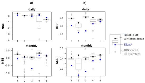
Figure 7.
Validation with discharge data for the chosen catchments. Nash-Sutcliffe Efficiency (NSE) (a) and Kling-Gupta Efficiency (KGE0 (b) for daily and monthly scales: all unique hydrotopes (boxplot) and catchment’s weighted mean (black square), ERA5 runoff as an additional reference (blue square).
The user might face the following limitations or problems applying the package. The biggest uncertainty obviously lies in the core of the framework—the global parameterization. The generalization of vegetation parameters could yield the same parameter set for completely different plant species united with one land cover class, e.g., vineyards and rice (cultivated territories), birch and teak (deciduous broadleaf forest). The same applies to soil hydraulic characteristics assigned based on texture class with values from local USA studies made by the initial model developers. Furthermore, it was found that land cover and soil rasters can have gaps. We observed a lack of consistency and accuracy in high latitudes and islands. This may be resolved in the near future (at least for the Global Land Cover) with the next annual update. Moreover, there are issues with the meteorological forcing dataset that should be considered. At present, with its long time-series, good spatiotemporal resolution, and large number of parameters available [99], ERA5 is one of the best and complete global-gridded reanalysis meteorological datasets [34,100,101,102,103]. However, its derived precipitation is still far from “state-of-the-art” conditions [104,105,106,107]. As a result, our validation implicitly showed that dataset resolution is still insufficient to capture precipitation heterogeneity in small catchments by smoothing flood peaks. Additionally, there is unfortunately always a chance that the data providers will change the download access interface, so that our retrieval code will need maintenance. There are also a few limitations caused by the BROOK90 itself [20], e.g., no implementation of flow routing, vegetation growth (aging), and snow frost. The first problem could be solved by adding a relatively simple bucket-type-routing module [108]. This will lead to a drastic increase of computation time, since one has to sacrifice the “unique-hydrotope subset” procedure, which significantly reduces model run time. On the other hand, this may serve well for small and relatively homogeneous catchments. Finally, regarding the package build-up itself, all problems presumably lie in the dependency and stability of the third-party R packages, the ERA5 server, and finally, absence currently of a user-friendly interface.
4. Conclusions and Outlook
This study describes a new R package, which integrates the lumped physical water balance model BROOK90 and open-source datasets within an automatic framework to calculate vertical water fluxes in soil–plant systems at any location on the globe.
The authors consider that the package presented could be beneficial and useful for several reasons. First, the package delivers reliable results for a vast number of water balance components in small catchments or at single sites. Second, the package enables the user to downscale some output variables of global hydrological reanalysis datasets (i.e., soil moisture, evapotranspiration, runoff) to the scale of a hydrotope. Furthermore, the simplicity of the package should encourage nonspecialists with limited or no prior knowledge of hydrological modeling, parameterization, calibration, etc. to simulate water balance components by following the simple guidelines. However, all users should be aware that the simulations and overall water balance estimations are subject to uncertainties and should be treated with caution. Finally, the package is setup to run globally; thus it could be especially valuable for water balance estimations in data-scarce regions, for instance, in regions with the lack or complete absence of hydrometeorological measurements or the inability to obtain reliable site characteristics.
Therefore, the package presented can serve for various applications and stakeholders. Besides detailed water balance analysis of small catchments with global applicability, possible implementations of the package include soil drought monitoring and water management in agriculture or forestry.
Future work will focus on a systematic global validation of the package, as well as on improvements regarding usability and incorporation of alternative datasets.
Author Contributions
Conceptualization, R.K. and I.V.; methodology, I.V. and R.K.; software, R.K. and I.V.; results, I.V.; writing—original draft preparation, I.V., writing—review, C.B. and R.K., writing—editing, I.V.; visualization, I.V.; supervision, R.K. All authors have read and agreed to the published version of the manuscript.
Funding
This research was funded by the German Federal Ministry of Education and Research (FKZ 01LR 2005A—funding measure “Regional Information on Climate Action” (RegIKlim), section (a) model regions.
Acknowledgments
Authors want to acknowledge developers and distributors of open-source data used in the study: Copernicus for ERA5 and Global Land Cover datasets, ISRIS for SoilGrids250m and GRDC for discharge data, and CRAN community for integrated R Packages. Additionally, authors thank both anonymous reviewers and the editor for the valuable comments on the manuscript.
Conflicts of Interest
The authors declare that they have no conflict of interest.
References
- Fekete, B.M.; Vörösmarty, C.J.; Grabs, W. High-resolution fields of global runoff combining observed river discharge and simulated water balances. Glob. Biogeochem. Cycles 2002, 16, 15-1–15-10. [Google Scholar] [CrossRef]
- Alfieri, L.; Burek, P.; Dutra, E.; Krzeminski, B.; Muraro, D.; Thielen, J.; Pappenberger, F. GloFAS—Global ensemble streamflow forecasting and flood early warning. Hydrol. Earth Syst. Sci. 2013, 17, 1161–1175. [Google Scholar] [CrossRef]
- Arheimer, B.; Pimentel, R.; Isberg, K.; Crochemore, L.; Andersson, J.; Hasan, A.; Pineda, L. Global catchment modelling using World-Wide HYPE (WWH), open data, and stepwise parameter estimation. Hydrol. Earth Syst. Sci. 2020, 24, 535–559. [Google Scholar] [CrossRef]
- Beck, H.E.; van Dijk, A.I.; De Roo, A.; Miralles, D.G.; McVicar, T.R.; Schellekens, J.; Bruijnzeel, L.A. Global-scale regionalization of hydrologic model parameters. Water Resour. Res. 2016, 52, 3599–3622. [Google Scholar] [CrossRef]
- Beck, H.E.; van Dijk, A.I.J.M.; de Roo, A.; Miralles, D.G.; McVicar, T.R.; Schellekens, J.; Bruijnzeel, L.A. Global evaluation of runoff from 10 state-of-the-art\hack\newline hydrological models. Hydrol. Earth Syst. Sci. 2017, 21, 2881–2903. [Google Scholar] [CrossRef]
- Döll, P.; Kaspar, F.; Lehner, B. A global hydrological model for deriving water availability indicators: Model tuning and validation. J. Hydrol. 2003, 270, 105–134. [Google Scholar] [CrossRef]
- Harrigan, S.; Zsoter, E.; Alfieri, L.; Prudhomme, C.; Salamon, P.; Wetterhall, F.; Barnard, C.; Cloke, H.; Pappenberger, F. GloFAS-ERA5 operational global river discharge reanalysis 1979–present. Earth Syst. Sci. Data Discuss. 2020, 2020, 1–23. [Google Scholar] [CrossRef]
- Qian, T.; Dai, A.; Trenberth, K.E.; Oleson, K.W. Simulation of Global Land Surface Conditions from 1948 to 2004. Part I: Forcing Data and Evaluations. J. Hydrometeorol. 2006, 7, 953–975. [Google Scholar] [CrossRef]
- Reichle, R.H.; Koster, R.D.; De Lannoy, G.J.; Forman, B.A.; Liu, Q.; Mahanama, S.P.; Touré, A. Assessment and Enhancement of MERRA Land Surface Hydrology Estimates. J. Clim. 2011, 24, 6322–6338. [Google Scholar] [CrossRef]
- Sood, A.; Smakhtin, V. Global hydrological models: A review. Hydrol. Sci. J. 2015, 60, 549–565. [Google Scholar] [CrossRef]
- Veldkamp, T.I.E.; Zhao, F.; Ward, P.J.; De Moel, H.; Aerts, J.C.; Schmied, H.M.; Portmann, F.T.; Masaki, Y.; Pokhrel, Y.; Liu, X.; et al. Human impact parameterizations in global hydrological models improve estimates of monthly discharges and hydrological extremes: A multi-model validation study. Environ. Res. Lett. 2018, 13, 055008. [Google Scholar] [CrossRef]
- Ebita, A.; Kobayashi, S.; Ota, Y.; Moriya, M.; Kumabe, R.; Onogi, K.; Harada, Y.; Yasui, S.; Miyaoka, K.; Takahashi, K.; et al. The Japanese 55-year Reanalysis “JRA-55”: An Interim Report. SOLA 2011, 7, 149–152. [Google Scholar] [CrossRef]
- Gelaro, R.; McCarty, W.; Suárez, M.J.; Todling, R.; Molod, A.; Takacs, L.; Randles, C.A.; Darmenov, A.; Bosilovich, M.G.; Reichle, R.; et al. The Modern-Era Retrospective Analysis for Research and Applications, Version 2 (MERRA-2). J. Clim. 2017, 30, 5419–5454. [Google Scholar] [CrossRef] [PubMed]
- Saha, S.; Moorthi, S.; Pan, H.-L.; Wu, X.; Wang, J.; Nadiga, S.; Tripp, P.; Kistler, R.; Woollen, J.; Behringer, D.; et al. The NCEP Climate Forecast System Reanalysis. Bull. Amer. Meteor. Soc. 2010, 91, 1015–1058. [Google Scholar] [CrossRef]
- Copernicus Climate Change Service (C3S). (2017): ERA5: Fifth Generation of ECMWF Atmospheric Reanalyses of the Global Climate, Copernicus Climate Change Service (C3S): ERA5: Fifth Generation of ECMWF Atmospheric Reanalyses of the Global Climate. ERA5 Hourly Data on Single Levels from 1979 to Present. 2018. Available online: https://cds.climate.copernicus.eu/cdsapp#!/dataset/reanalysis-era5-single-levels?tab=form (accessed on 14 February 2020).
- Wood, E.F.; Roundy, J.K.; Troy, T.J.; Van Beek, L.P.H.; Bierkens, M.F.; Blyth, E.; de Roo, A.; Döll, P.; Ek, M.; Famiglietti, J.; et al. Hyperresolution global land surface modeling: Meeting a grand challenge for monitoring Earth’s terrestrial water. Water Resour. Res. 2011, 47. [Google Scholar] [CrossRef]
- Collenteur, R. Open Source Python Packages in Hydrology. 2020. Available online: https://github.com/raoulcollenteur/Python-Hydrology-Tools (accessed on 18 February 2020).
- Slater, L.J.; Thirel, G.; Harrigan, S.; Delaigue, O.; Hurley, A.; Khouakhi, A.; Prosdocimi, I.; Vitolo, C.; Smith, K. Using R in hydrology: A review of recent developments and future directions. Hydrol. Earth Syst. Sci. 2019, 23, 2939–2963. [Google Scholar] [CrossRef]
- Box, G.E.P.; Draper, N.R. Empirical Model-Building and Response Surfaces; John Wiley & Sons: Oxford, UK, 1987. [Google Scholar]
- Federer, C.A. BROOK 90: A simulation model for evaporation, soil water, and streamflow. 2002. Available online: http://www.ecoshift.net/brook/brook90.htm (accessed on 2 June 2020).
- Buchhorn, M.; Lesiv, M.; Tsendbazar, N.E.; Herold, M.; Bertels, L.; Smets, B. Copernicus Global Land Service: Land Cover 100 m, epoch “year”, Globe (Version V2.0.2). 2019. Available online: https://zenodo.org/record/3243509#.XxFzWcfVLIU (accessed on 14 February 2020).
- Hengl, T.; Mendes de Jesus, J.; Heuvelink, G.B.; Ruiperez Gonzalez, M.; Kilibarda, M.; Blagotić, A.; Shangguan, W.; Wright, M.N.; Geng, X.; Bauer-Marschallinger, B.; et al. SoilGrids250m: Global gridded soil information based on machine learning. PLoS ONE 2017, 12, 1–40. [Google Scholar] [CrossRef]
- Federer, C.A.; Vörösmarty, C.; Fekete, B. Sensitivity of Annual Evaporation to Soil and Root Properties in Two Models of Contrasting Complexity. J. Hydrometeorol. 2003, 4, 1276–1290. [Google Scholar] [CrossRef]
- Kronenberg, R.; Oehlschlägel, L.M. BROOK90 in R. 2019. Available online: https://github.com/rkronen/Brook90_R (accessed on 2 June 2020).
- Carr, A.E.; Loague, K.; VanderKwaak, J.E. Hydrologic-response simulations for the North Fork of Caspar Creek: Second-growth, clear-cut, new-growth, and cumulative watershed effect scenarios. Hydrol. Process. 2014, 28, 1476–1494. [Google Scholar] [CrossRef]
- Felsmann, K.; Baudis, M.; Kayler, Z.E.; Puhlmann, H.; Ulrich, A.; Gessler, A. Responses of the structure and function of the understory plant communities to precipitation reduction across forest ecosystems in Germany. Ann. For. Sci. 2017, 75, 3. [Google Scholar] [CrossRef]
- Kremsa, J.; Křeček, J.; Kubin, E. Comparing the impacts of mature spruce forests and grasslands on snow melt, water resource recharge, and run-off in the northern boreal environment. Int. Soil Water Conserv. Res. 2015, 3, 50–56. [Google Scholar] [CrossRef]
- Luong, T.T.; Kronenberg, R.; Lorenz, J.; Bernhofer, C. Deriving rainfall thresholds based on soil moisture conditions for flash flood warning in a forested catchment using a physical process-based model. In Geophysical Research Abstracts; EGU General Assembly: Vienna, Austria, 2018; p. 20. Available online: https://meetingorganizer.copernicus.org/EGU2018/EGU2018-4747.pdf (accessed on 17 July 2020).
- Vilhar, U. Comparison of drought stress indices in beech forests: A modelling study. iFor. Biogeosci. For. 2016, 635–642. [Google Scholar] [CrossRef]
- Hufkens, K.; Stauffer, R.; Campitelli, E. Programmatic interface to the two European Centre for Medium-Range Weather Forecasts API services; Version v1.2.0; CRAN: Vienna, Austria, 2020. [Google Scholar]
- Copernicus Climate Change Service Information. ERA5 Documentation. 2020. Available online: https://confluence.ecmwf.int/display/CKB/ERA5%3A+data+documentation (accessed on 13 February 2020).
- Hersbach, H.; Dee, D. ERA5 reanalysis is in production. 2016. Available online: https://www.ecmwf.int/sites/default/files/elibrary/2016/16299-newsletter-no147-spring-2016.pdf (accessed on 14 February 2020).
- Martens, B.; Schumacher, D.L.; Wouters, H.; Muñoz-Sabater, J.; Verhoest, N.E.C.; Miralles, D.G. Evaluating the surface energy partitioning in ERA5. Geosci. Model Dev. Discuss. 2020, 2020, 1–35. [Google Scholar] [CrossRef]
- Tarek, M.; Brissette, F.P.; Arsenault, R. Evaluation of the ERA5 reanalysis as a potential reference dataset for hydrological modelling over North-America. Hydrol. Earth Syst. Sci. Discuss. 2020, 24, 2527–2544. [Google Scholar] [CrossRef]
- Tetzner, D.; Thomas, E.; Allen, C. A Validation of ERA5 Reanalysis Data in the Southern Antarctic Peninsula—Ellsworth Land Region, and Its Implications for Ice Core Studies. Geosciences 2019, 9. [Google Scholar] [CrossRef]
- Vitart, F.; Balsamo, G.; Bidlot, J.; Lang, S.; Tsonevsky, I.; Richardson, D.; Balmaseda, M. Use of ERA5 reanalysis to initialise re-forecasts proves beneficial. 2019. Available online: https://www.ecmwf.int/en/newsletter/161/meteorology/use-era5-reanalysis-initialise-re-forecasts-proves-beneficial (accessed on 14 February 2020).
- Vorobevskii, I.; Kronenberg, R. Geoserver TU Dresden2020. Available online: http://141.76.16.238:8080/geoserver/ (accessed on 17 July 2020).
- Dai, Y.; Shangguan, W.; Wei, N.; Xin, Q.; Yuan, H.; Zhang, S.; Liu, S.; Lu, X.; Wang, D.; Yan, F. A review of the global soil property maps for Earth system models. SOIL 2019, 5, 137–158. [Google Scholar] [CrossRef]
- Ross, C.W.; Prihodko, L.; Anchang, J.Y.; Kumar, S.S.; Ji, W.; Hanan, N.P. HYSOGs250m, global gridded hydrologic soil groups for curve-number-based runoff modeling. Sci. Data 2018, 5, 180091. [Google Scholar] [CrossRef]
- Okello, A.M.L.S.; Masih, I.; Uhlenbrook, S.; Jewitt, G.P.W.; van der Zaag, P. Improved Process Representation in the Simulation of the Hydrology of a Meso-Scale Semi-Arid Catchment. Water 2018, 10. [Google Scholar] [CrossRef]
- Stoorvogel, J.J.; Mulder, V.L.; Hendriks, C.M.J. The effect of disaggregating soil data for estimating soil hydrological parameters at different scales. Geoderma 2019, 347, 185–193. [Google Scholar] [CrossRef]
- Umer, Y.M.; Jetten, V.G.; Ettema, J. Sensitivity of flood dynamics to different soil information sources in urbanized areas. J. Hydrol. 2019, 577, 123945. [Google Scholar] [CrossRef]
- Moumen, Z.; Nabih, S.; Elhassnaoui, I.; Lahrach, A. Hydrologic Modeling Using SWAT: Test the Capacity of SWAT Model to Simulate the Hydrological Behavior of Watershed in Semi-Arid Climate. In Decision Support Methods for Assessing Flood Risk and Vulnerability; IGI Global: Hershey, PA, USA, 2020; pp. 162–198. [Google Scholar] [CrossRef]
- Buchhorn, M.; Lesiv, M.; Tsendbazar, N.-E.; Herold, M.; Bertels, L.; Smets, B. Copernicus Global Land Cover Layers—Collection 2. Remote Sens. 2020, 12, 1044. [Google Scholar] [CrossRef]
- Buchhorn, M.; Smets, B.; Bertels, L.; Lesiv, M.; Tsendbazar, N.-E. Product user manual. Moderate dynamic land cover 100 m. Version 2. Copernicus Global Land Operations “Vegetation and Energy”, I2.10. 2019. Available online: https://land.copernicus.eu/global/sites/cgls.vito.be/files/products/CGLOPS1_PUM_LC100m-V2.0_I2.20.pdf (accessed on 16 July 2020).
- Buchhorn, M.; Lesiv, M.; Tsendbazar, N.E.; Herold, M.; Bertels, L.; Smets, B. Download page for Copernicus Global Land Service: Land Cover 100 m, 20 × 20 degree tiles. 2019. Available online: https://github.com/cgls/LandCoverDownloader/blob/master/list_url.txt (accessed on 14 February 2020).
- Tsendbazar, N.E.; Herold, M.; De Bruin, S.; Lesiv, M.; Fritz, S.; Van De Kerchove, R.; Buchhorn, M.; Duerauer, M.; Szantoi, Z.; Pekel, J.F. Developing and applying a multi-purpose land cover validation dataset for Africa. Remote Sens. Environ. 2018, 219, 298–309. [Google Scholar] [CrossRef]
- Tsendbazar, N.E.; Herold, M.; Tarko, A.; Li, L.; Lesiv, M.; Fritz, S. Validation report. Moderate dynamic land cover 100 m. Version 2. Copernicus Global Land Operations “Vegetation and Energy”, I1.00. 2019. Available online: https://land.copernicus.eu/global/sites/cgls.vito.be/files/products/CGLOPS1_VR_LC100m-V2.0_I1.00.pdf (accessed on 16 July 2020).
- European Space Agency. Land Cover CCI Product User Guide Version 2. 2017. Available online: http://maps.elie.ucl.ac.be/CCI/viewer/download/ESACCI-LC-Ph2-PUGv2_2.0.pdf (accessed on 17 April 2020).
- Sulla-Menashe, D.; Friedl, M. MCD12Q1 MODIS/Terra+Aqua Land Cover Type Yearly L3 Global 500 m SIN Grid V006; NASA EOSDIS Land Processes DAAC: Sioux Falls, SD, USA, 2019.
- Bartholomé, E.; Belward, A.S. GLC2000: A new approach to global land cover mapping from Earth observation data. Int. J. Remote Sens. 2005, 26, 1959–1977. [Google Scholar] [CrossRef]
- Jun, C.; Ban, Y.; Li, S. Open access to Earth land-cover map. Nature 2014, 514, 434. [Google Scholar] [CrossRef] [PubMed]
- Hollister, J.; Shah, T. Elevatr: Access Elevation Data from Various APIs; CRAN: Vienna, Austria, 2017. [Google Scholar]
- U.S. Geological Survey (USGS) National Geospatial Program. 3D Elevation Program. 2020. Available online: https://www.usgs.gov/core-science-systems/ngp/3dep (accessed on 17 April 2020).
- Porter, C.; Morin, P.; Howat, I.; Noh, M.J.; Bates, B.; Peterman, K.; Keesey, S.; Schlenk, M.; Gardiner, J.; Tomko, K.; et al. ‘ArcticDEM’. Harvard Dataverse; Polar Geospatial Center: Saint Paul, MN, USA, 2018. [Google Scholar] [CrossRef]
- Natural Resources Canada. Canadian Digital Elevation Model. 2019. Available online: https://open.canada.ca/data/en/dataset/7f245e4d-76c2-4caa-951a-45d1d2051333 (accessed on 17 April 2020).
- Government Digital Service. Find Open Data. 2020. Available online: https://data.gov.uk (accessed on 17 April 2020).
- Bundesministerium für Digitalisierung, und Wirtschaftsstandort, and Government Digital Service. Offene Daten Österreichs. 2020. Available online: https://www.data.gv.at/ (accessed on 17 April 2020).
- Amante, C.; Eakins, B.W. ETOPO1: 1 Arc-Minute Global Relief Model: Procedures, Data Sources and Analysis. NOAA Technical Memorandum NESDIS NGDC-24. 2009. Available online: https://www.ngdc.noaa.gov/mgg/global/relief/ETOPO1/docs/ETOPO1.pdf (accessed on 17 April 2020).
- European Environment Agency (EEA) under the Framework of the Copernicus Programme. European Digital Elevation Model (EU-DEM), Version 1.1. 2016. Available online: https://land.copernicus.eu/imagery-in-situ/eu-dem/eu-dem-v1.1/view (accessed on 17 April 2020).
- Danielson, J.J.; Gesch, D.B. Global Multi-Resolution Terrain Elevation Data 2010 (GMTED2010): U.S. Geological Survey Open-File Report. 2011. Available online: https://pubs.usgs.gov/of/2011/1073/pdf/of2011-1073.pdf (accessed on 17 July 2020).
- Instituto Nacional de Estadística, Geografía e Informática. Continuo de Elevaciones Mexicano (CEM). 2013. Available online: https://www.inegi.org.mx/app/geo2/elevacionesmex/ (accessed on 17 April 2020).
- Norwegian Mapping Authority, Mapping and Cadastre. Kartverket: Open and Free Geospatial Data from Norway. 2020. Available online: https://www.kartverket.no/en/data/Open-and-Free-geospatial-data-from-Norway/ (accessed on 17 April 2020).
- Land Information New Zealand (LINZ). LINZ Data Service: LiDAR 1 m DEM. 2020. Available online: https://data.linz.govt.nz (accessed on 17 April 2020).
- NASA JPL. NASA Shuttle Radar Topography Mission Global 1 arc second [Data set]; NASA EOSDIS Land Processes DAAC: Sioux Falls, SD, USA, 2019. [CrossRef]
- OpenStreetMap Contributors. Planet Dump. 2019. Available online: https://www.openstreetmap.org (accessed on 17 July 2020).
- Bougeault, P. Cloud-Ensemble Relations Based on the Gamma Probability Distribution for the Higher-Order Models of the Planetary Boundary Layer. J. Atmos. Sci. 1982, 39, 2691–2700. [Google Scholar] [CrossRef]
- Bonan, G.B.; Levis, S.; Kergoat, L.; Oleson, K.W. Landscapes as patches of plant functional types: An integrating concept for climate and ecosystem models. Glob. Biogeochem. Cycles 2002, 16, 5-1–5-23. [Google Scholar] [CrossRef]
- Jackson, R.B.; Canadell, J.; Ehleringer, J.R.; Mooney, H.A.; Sala, O.E.; Schulze, E.D. A global analysis of root distributions for terrestrial biomes. Oecologia 1996, 108, 389–411. [Google Scholar] [CrossRef]
- Körner, C.H. Leaf Diffusive Conductances in the Major Vegetation Types of the Globe. In Ecophysiology of Photosynthesis; Schulze, E.-D., Caldwell, M.M., Eds.; Springer: Berlin/Heidelberg, Germany, 1995; pp. 463–490. [Google Scholar]
- Newman, E.; Carson, E. The Plant Root and Its Environment; Carlson, E.W., Ed.; University Press of Virginia: Charlottesville, VA, USA, 1974; pp. 363–440. [Google Scholar]
- Safford, L.O.; Bell, S. Biomass of Fine Roots in a White Spruce Plantation. Can. J. For. Res. 1972, 2, 169–172. [Google Scholar] [CrossRef]
- Safford, L.O. Effect of fertilization on biomass and nutrient content of fine roots in a beech-birch-maple stand. Plant Soil 1974, 40, 349–363. [Google Scholar] [CrossRef]
- R Core Team. R: A Language and Environment for Statistical Computing; R Foundation for Statistical Computing: Vienna, Austria, 2019. [Google Scholar]
- RStudio Team. RStudio: Integrated Development Environment for R; RStudio, Inc.: Boston, MA, USA, 2016. [Google Scholar]
- Vorobevskii, I.; Kronenberg, R. Global BROOK90. 2020. Available online: https://github.com/hydrovorobey/Global_BROOK90 (accessed on 22 June 2020).
- Rinker, T.W.; Kurkiewicz, D. pacman: Package Management for R; CRAN: Vienna, Austria, 2018. [Google Scholar]
- Hijmans, R.J. Raster: Geographic Data Analysis and Modeling; CRAN: Vienna, Austria, 2019. [Google Scholar]
- Bivand, R.; Keitt, T.; Rowlingson, B. Rgdal: Bindings for the ‘Geospatial’ Data Abstraction Library; CRAN: Vienna, Austria, 2018. [Google Scholar]
- Bivand, R.S.; Pebesma, E.; Gomez-Rubio, V. Applied Spatial Data Analysis with R, 2nd ed.; Springer: New York, NY, USA, 2013. [Google Scholar]
- Csárdi, G. Keyring: Access the System Credential Store from R; CRAN: Vienna, Austria, 2018. [Google Scholar]
- Grolemund, G.; Wickham, H. Dates and Times Made Easy with lubridate. J. Stat. Softw. 2011, 40, 1–25. [Google Scholar] [CrossRef]
- Bivand, R.; Rundel, C. Rgeos: Interface to Geometry Engine—Open Source (‘GEOS’); CRAN: Vienna, Austria, 2018. [Google Scholar]
- Wickham, H. Stringr: Simple, Consistent Wrappers for Common String Operations; CRAN: Vienna, Austria, 2018. [Google Scholar]
- Wickham, H. The Split-Apply-Combine Strategy for Data Analysis. J. Stat. Softw. 2011, 40, 1–29. [Google Scholar] [CrossRef]
- Dowle, M.; Srinivasan, A. Data.Table: Extension of Data.Frame; CRAN: Vienna, Austria, 2018. [Google Scholar]
- Pierce, D. ncdf4: Interface to Unidata netCDF (Version 4 or Earlier) Format Data Files; CRAN: Vienna, Austria, 2017. [Google Scholar]
- Teucher, A. Lutz: Look up Time Zones of Point Coordinates; CRAN: Vienna, Austria, 2019. [Google Scholar]
- Wickham, H. ggplot2: Elegant Graphics for Data Analysis; Springer: New York, NY, USA, 2016. [Google Scholar]
- Federal Institute of Hydrology. The GRDC—The World-Wide Repository of River Discharge Data and Associated Metadata. 2020. Available online: https://www.bafg.de/GRDC/EN/Home/homepage_node.html (accessed on 16 February 2020).
- Kottek, M.; Grieser, J.; Beck, C.; Rudolf, B.; Rubel, F. World Map of the Köppen-Geiger climate classification updated. Meteorol. Z. 2006, 15, 259–263. [Google Scholar] [CrossRef]
- Microsoft. BingTM Maps Tiles. 2020. Available online: http://ecn.t3.tiles.virtualearth.net/tiles/a{q}.jpeg?g=1 (accessed on 15 February 2020).
- Vargas, R. Digital Soil Map of the World; FAO-UN—Land and Water Division: Rome, Italy, 2007. [Google Scholar]
- Balsamo, G.; Beljaars, A.; Scipal, K.; Viterbo, P.; van den Hurk, B.; Hirschi, M.; Betts, A.K. A Revised Hydrology for the ECMWF Model: Verification from Field Site to Terrestrial Water Storage and Impact in the Integrated Forecast System. J. Hydrometeor. 2009, 10, 623–643. [Google Scholar] [CrossRef]
- Earth Resources Observation and Science (EROS) Center. USGS EROS Archive-Land Cover Products-Global Land Cover Characterization (GLCC); EROS Center: Sioux Falls, SD, USA, 1997.
- ECMWF. Part IV: Physical Processes. In IFS Documentation CY41R2; ECMWF: Reading, UK, 2016. [Google Scholar]
- Nash, J.E.; Sutcliffe, J.V. River flow forecasting through conceptual models part I—A discussion of principles. J. Hydrol. 1970, 10, 282–290. [Google Scholar] [CrossRef]
- Gupta, H.V.; Kling, H.; Yilmaz, K.K.; Martinez, G.F. Decomposition of the mean squared error and NSE performance criteria: Implications for improving hydrological modelling. J. Hydrol. 2009, 377, 80–91. [Google Scholar] [CrossRef]
- Atmospheric Circulation Reconstructions over the Earth Initiative, Global Climate Observing System (GCOS) Working Group on Surface Pressure, and World Climate Research Programme, Advancing Reanalysis: Atmospheric Reanalyses Comparison Table. 2020. Available online: https://reanalyses.org (accessed on 16 April 2020).
- Balsamo, G.; Dutra, E.; Albergel, C.; Munier, S.; Calvet, J.C.; Munoz-Sabater, J.; de Rosnay, P. ERA-5 and ERA-Interim driven ISBA land surface model simulations: Which one performs better? Hydrol. Earth Syst. Sci. 2018, 22, 3515–3532. [Google Scholar] [CrossRef]
- Malakar, P.; Kesarkar, A.P.; Bhate, J.N.; Singh, V.; Deshamukhya, A. Comparison of Reanalysis Data Sets to Comprehend the Evolution of Tropical Cyclones Over North Indian Ocean. Earth Space Sci. 2020, 7, e2019EA000978. [Google Scholar] [CrossRef]
- Ramon, J.; Lledó, L.; Torralba, V.; Soret, A.; Doblas-Reyes, F.J. What global reanalysis best represents near-surface winds? Q. J. R. Meteorol. Soc. 2019, 145, 3236–3251. [Google Scholar] [CrossRef]
- Urraca, R.; Huld, T.; Gracia-Amillo, A.; Martinez-de-Pison, F.J.; Kaspar, F.; Sanz-Garcia, A. Evaluation of global horizontal irradiance estimates from ERA5 and COSMO-REA6 reanalyses using ground and satellite-based data. Sol. Energy 2018, 164, 339–354. [Google Scholar] [CrossRef]
- Fallah, A.; Rakhshandehroo, G.R.; Berg, P.; O, S.; Orth, R. Evaluation of precipitation datasets against local observations in southwestern Iran. Int. J. Climatol. 2019. [Google Scholar] [CrossRef]
- Sharifi, E.; Eitzinger, J.; Dorigo, W. Performance of the State-Of-The-Art Gridded Precipitation Products over Mountainous Terrain: A Regional Study over Austria. Remote Sens. 2019, 11, 2018. [Google Scholar] [CrossRef]
- Xu, X.; Frey, S.K.; Boluwade, A.; Erler, A.R.; Khader, O.; Lapen, D.R.; Sudicky, E. Evaluation of variability among different precipitation products in the Northern Great Plains. J. Hydrol. Reg. Stud. 2019, 24, 100608. [Google Scholar] [CrossRef]
- Zandler, H.; Haag, I.; Samimi, C. Evaluation needs and temporal performance differences of gridded precipitation products in peripheral mountain regions. Sci. Rep. 2019, 9, 15118. [Google Scholar] [CrossRef] [PubMed]
- Santos, L.; Thirel, G.; Perrin, C. Continuous state-space representation of a bucket-type rainfall-runoff model: A case study with the GR4 model\hack\break using state-space GR4 (Version 1.0). Geosci. Model Dev. 2018, 11, 1591–1605. [Google Scholar] [CrossRef]
© 2020 by the authors. Licensee MDPI, Basel, Switzerland. This article is an open access article distributed under the terms and conditions of the Creative Commons Attribution (CC BY) license (http://creativecommons.org/licenses/by/4.0/).