Modelling Projected Changes in Soil Water Budget in Coastal Kenya under Different Long-Term Climate Change Scenarios

 ,
,  ,
,  ,
, 
 and
and 
Abstract
:1. Introduction
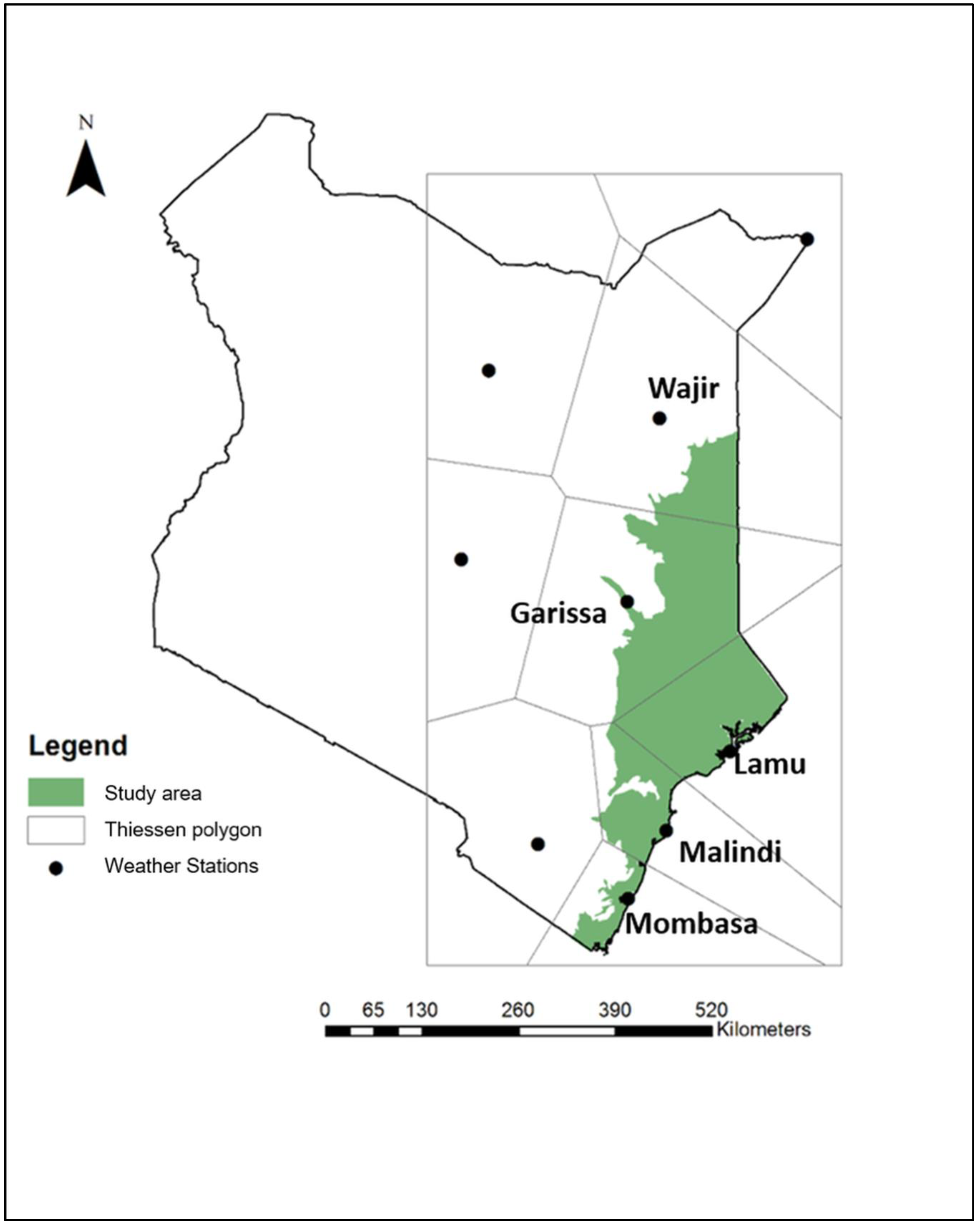
Study Area
2. Materials and Methods
2.1. Model Input
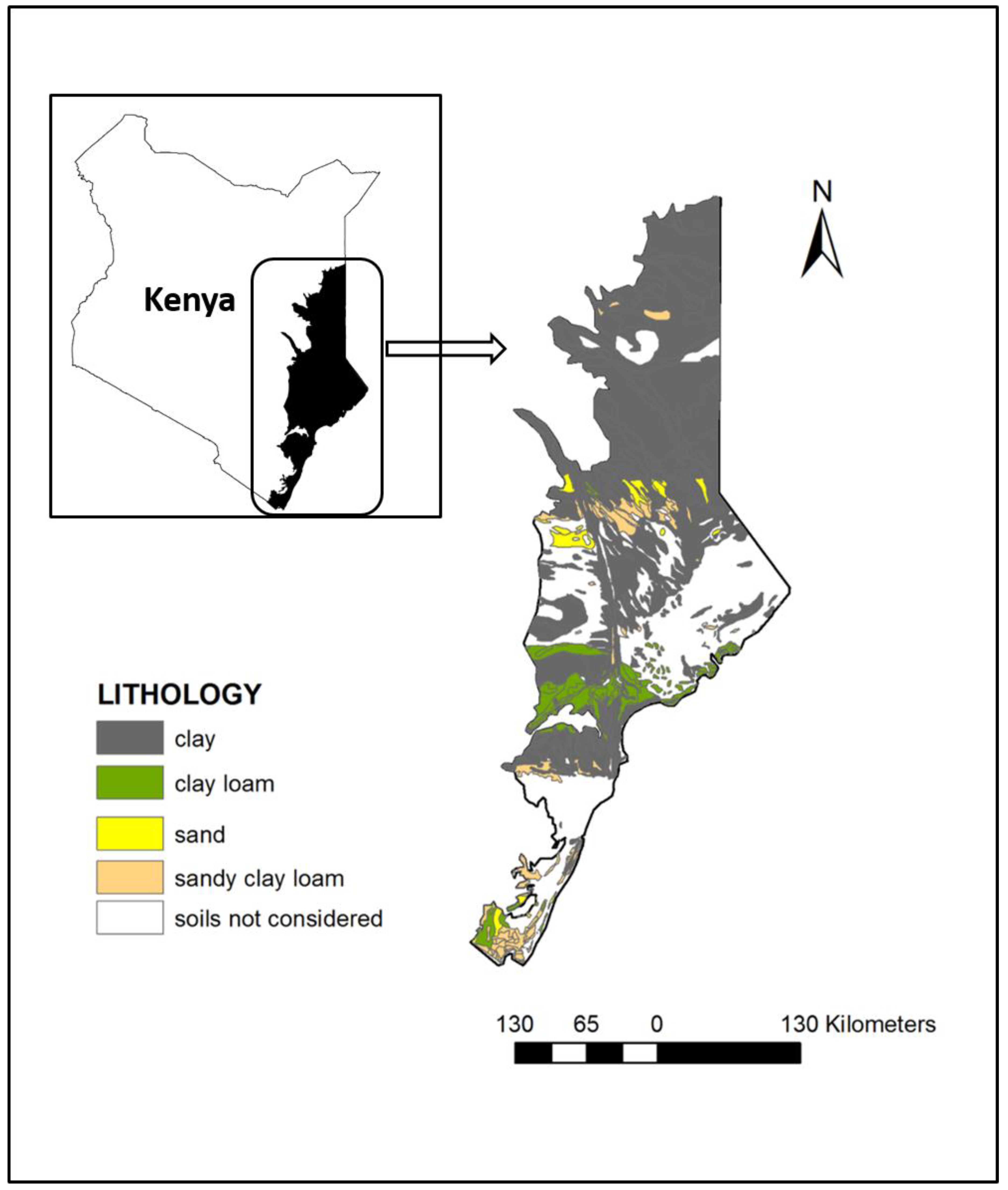
2.1.1. Soils
2.1.2. Climate Data
3. Results
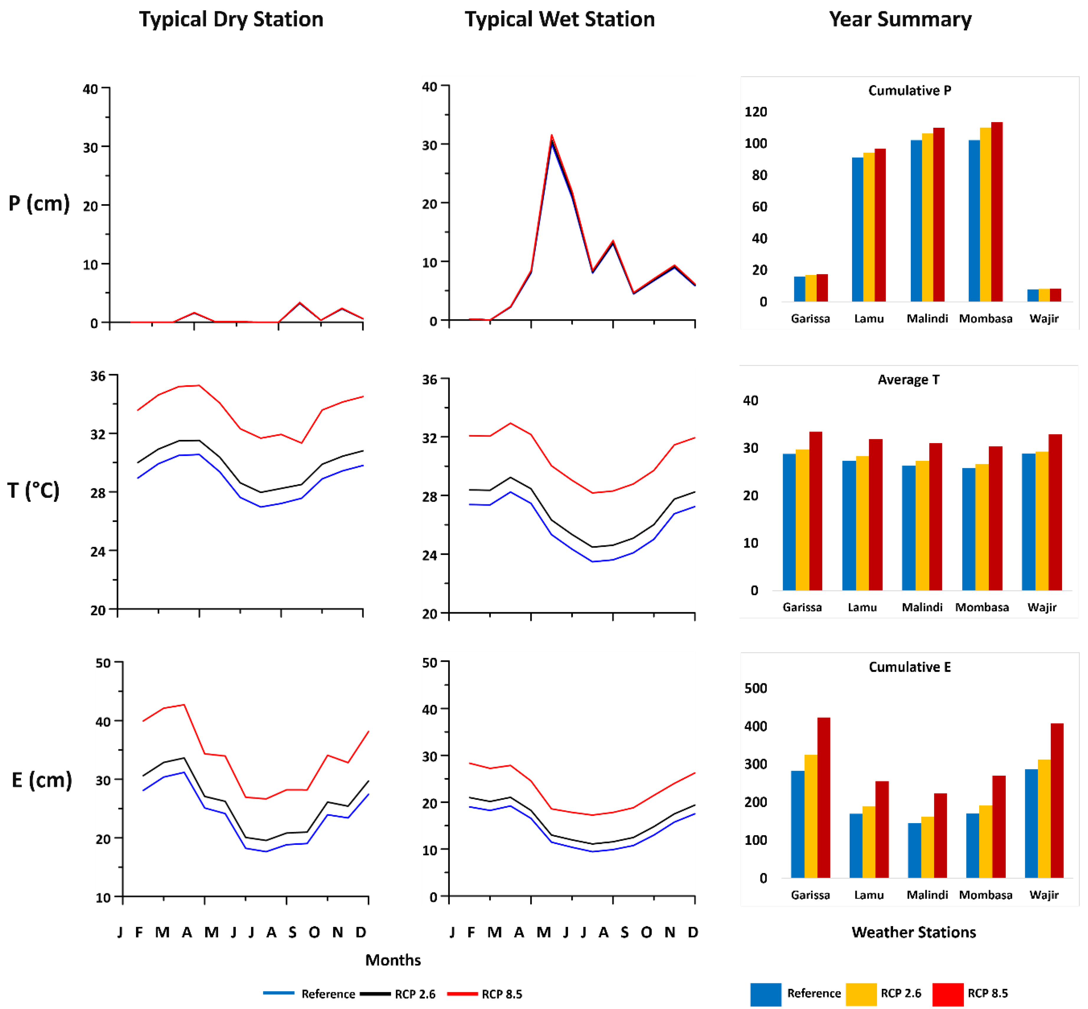
3.1. Climate Data
3.2. Simulation Results
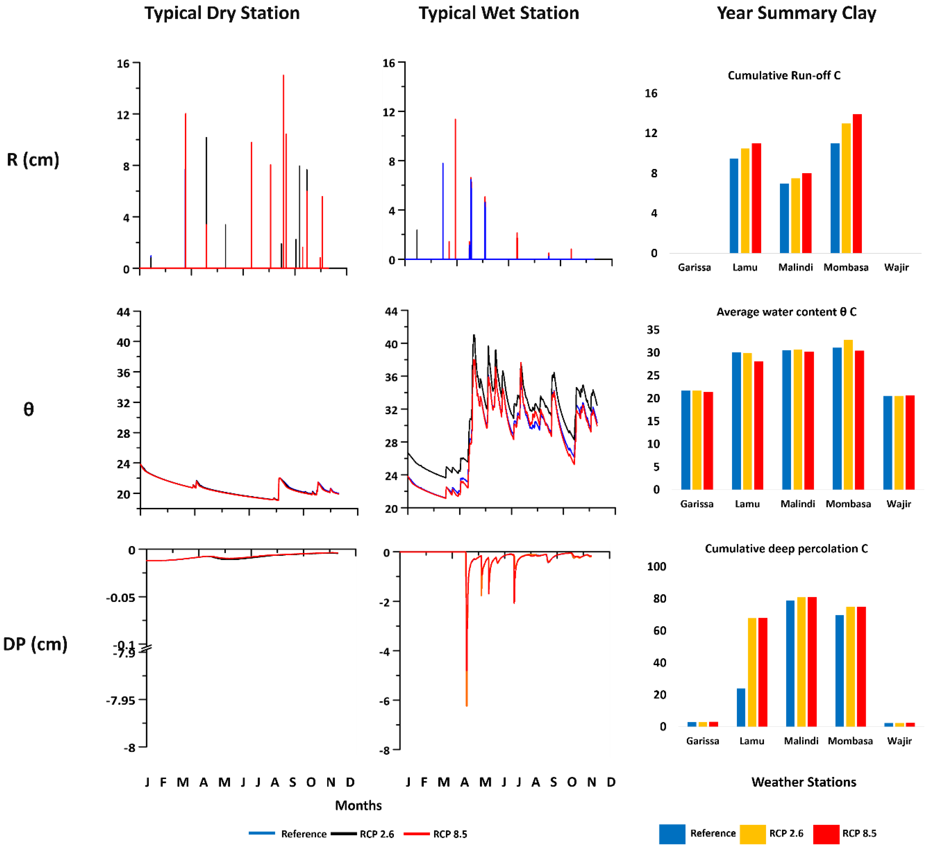
3.2.1. Clay Soils
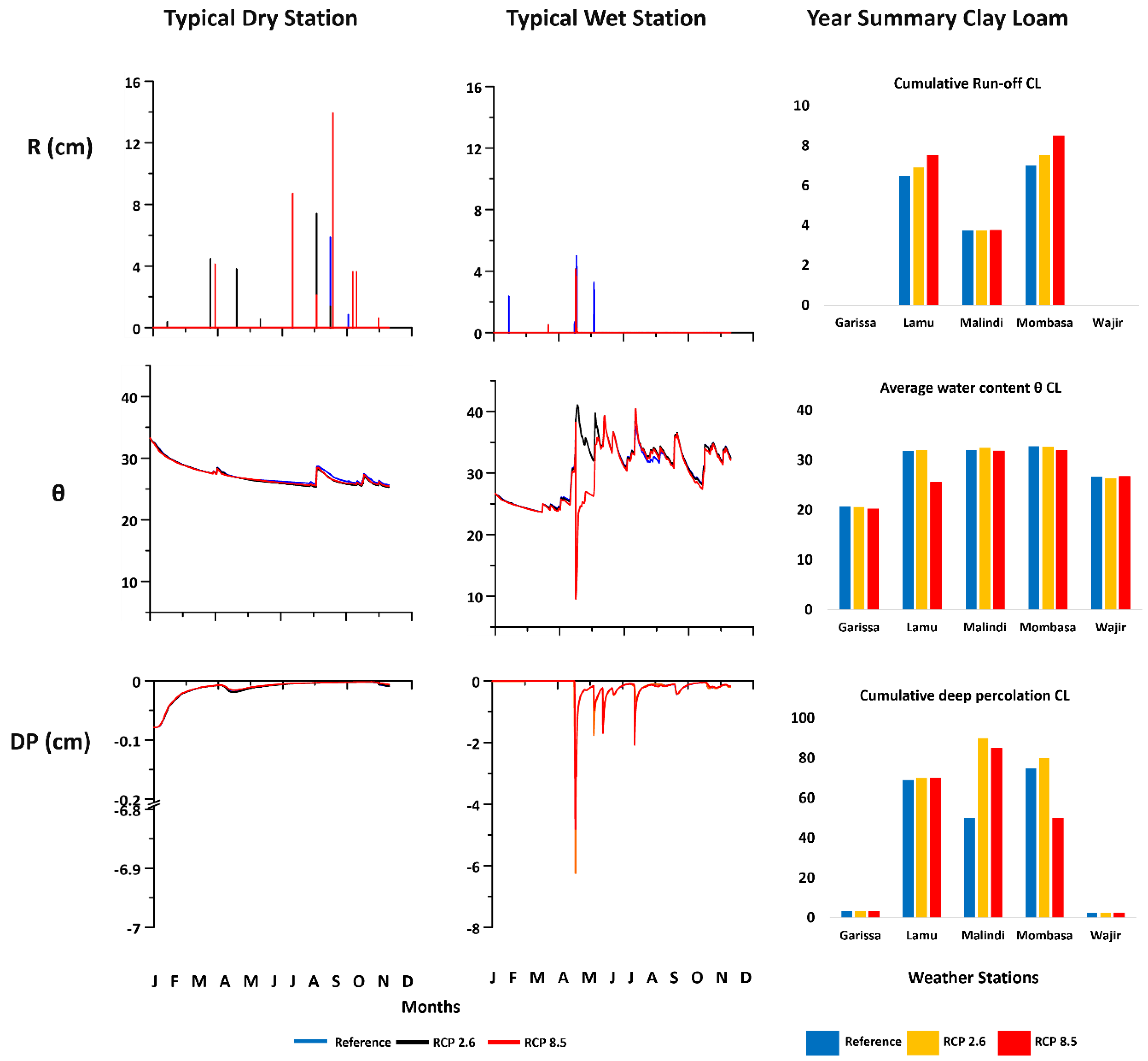
3.2.2. Clay Loam Soils
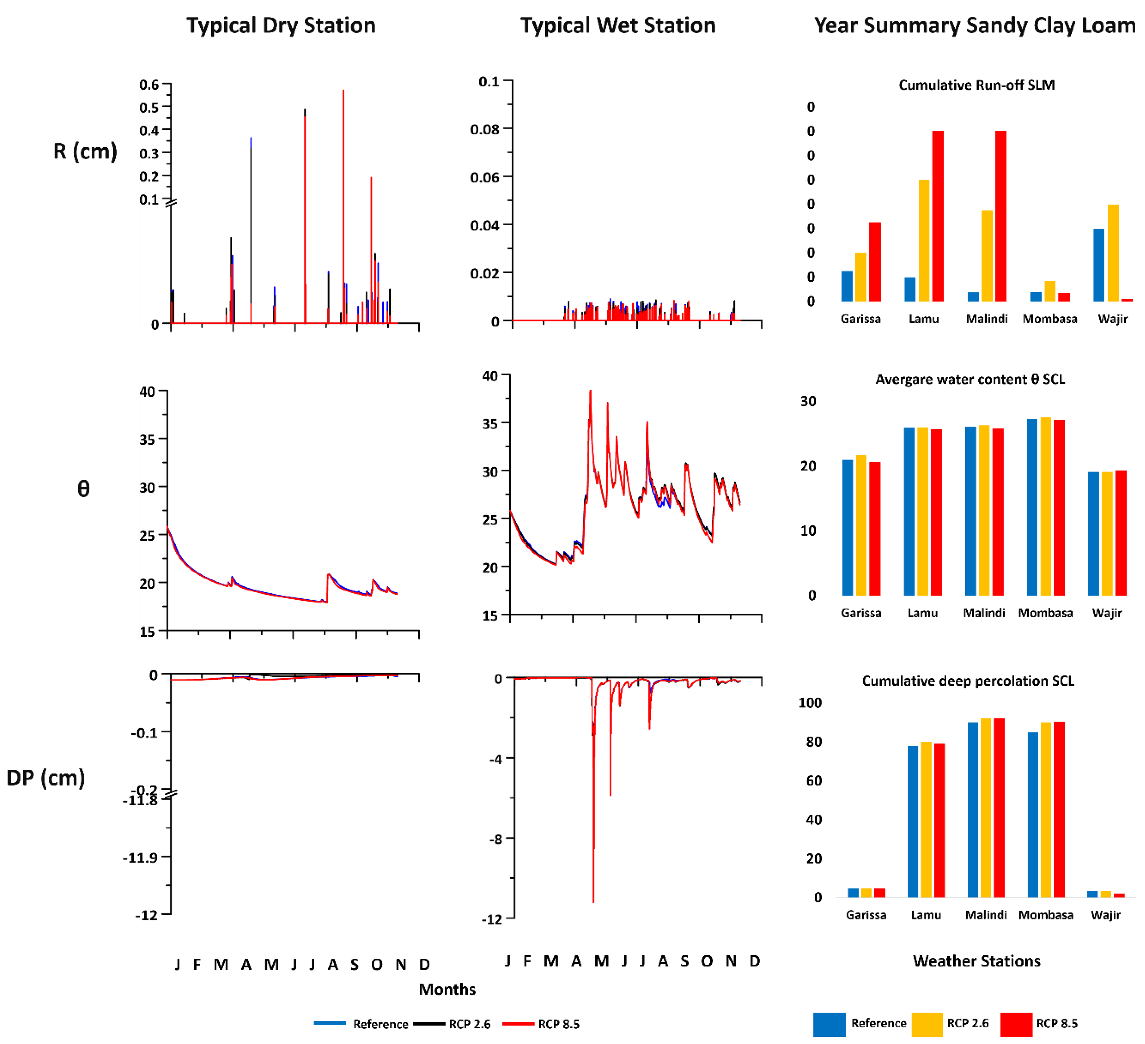
3.2.3. Sandy Clay Loam Soils
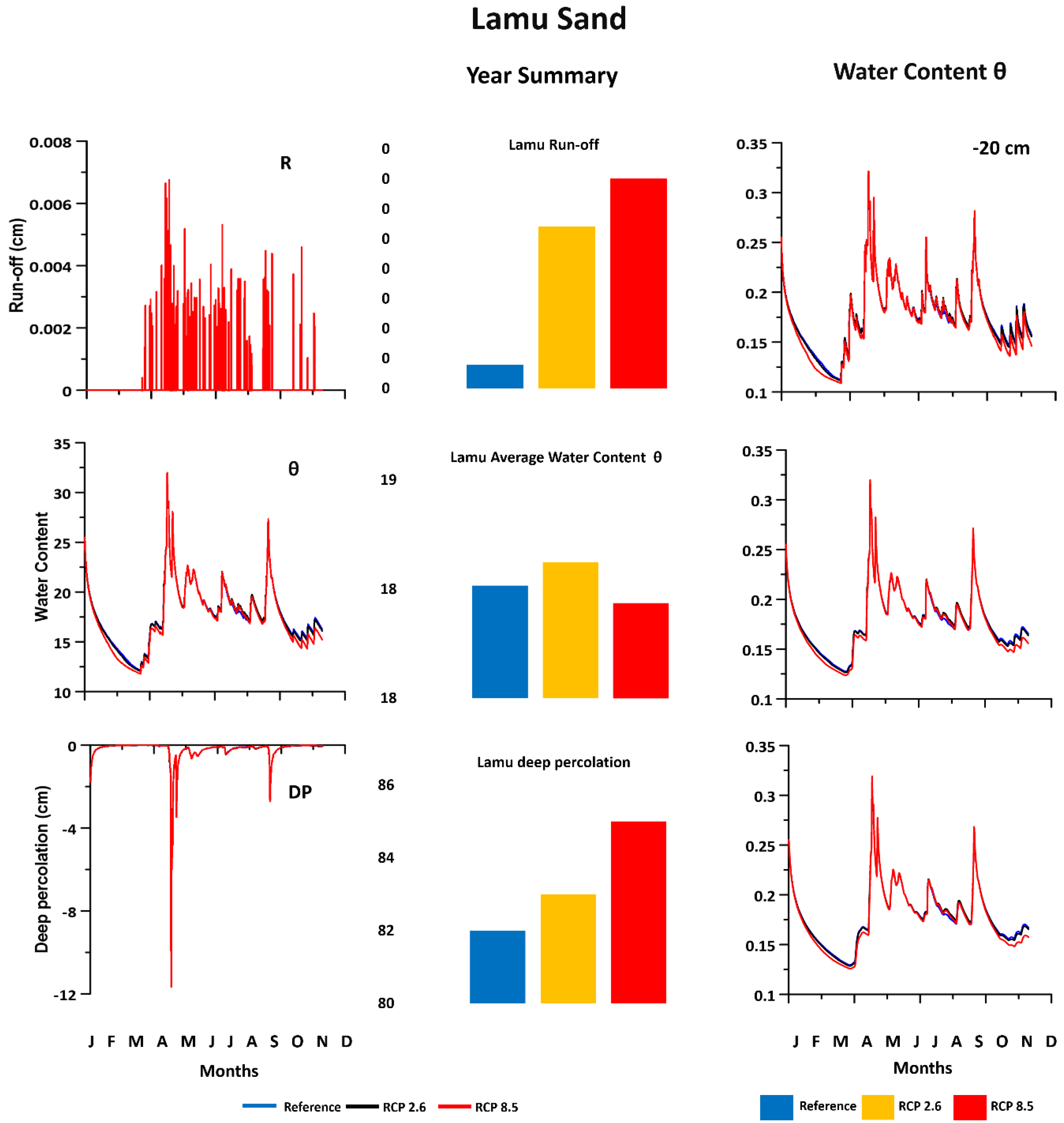
3.2.4. Sandy Soils (Lamu)
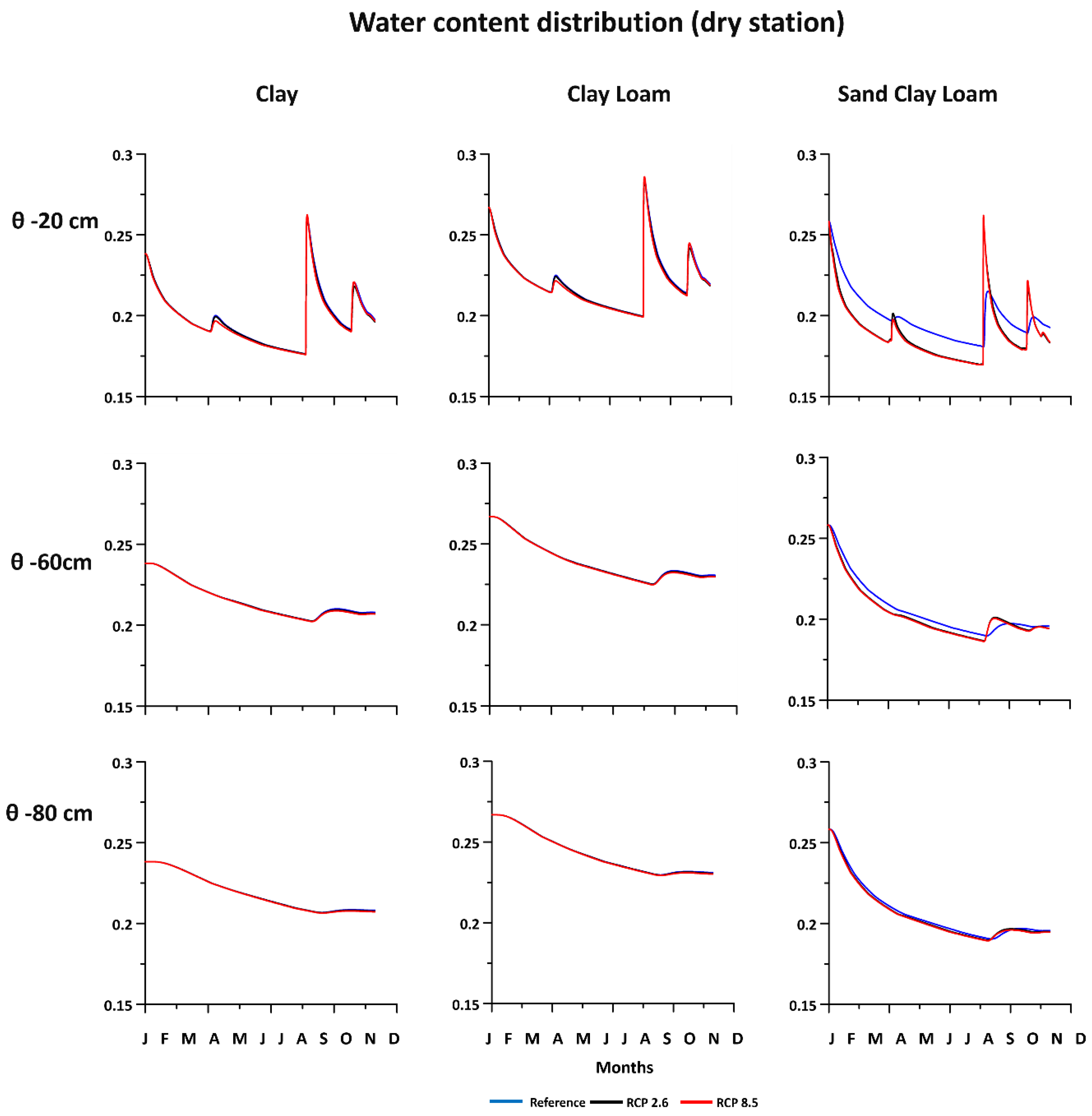
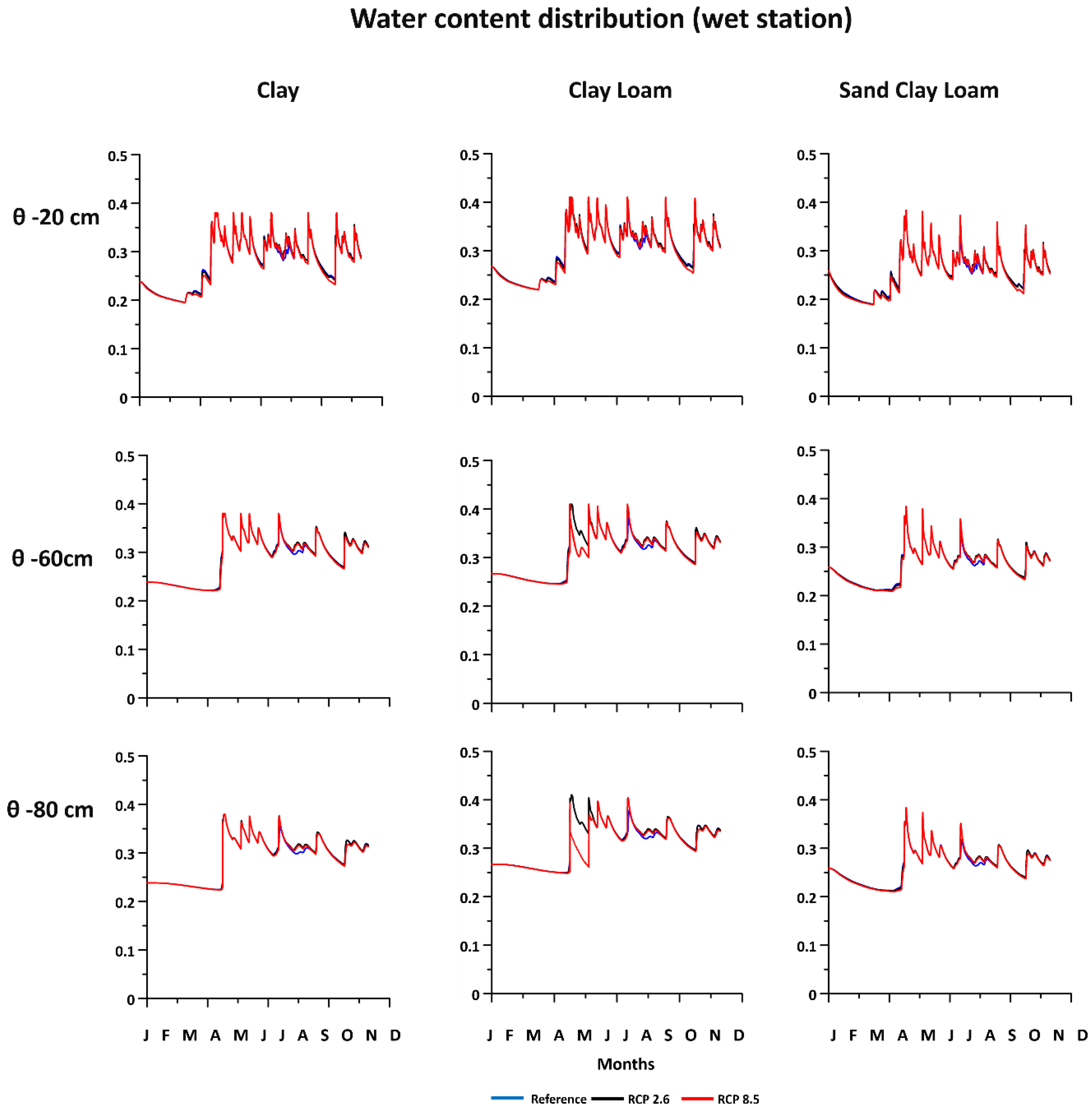
3.2.5. Water Content at Various Depths in the Soil Column
3.2.6. Water Budget per Weather Station
3.2.7. Climate Change Scenarios
4. Discussion
5. Conclusions and Recommendations
Author Contributions
Funding
Acknowledgments
Conflicts of Interest
References
- Barquero, F.; Fichtner, T.; Stefan, C. Methods of in situ assessment of infiltration rate reduction in groundwater recharge basins. Water 2019, 11, 784. [Google Scholar] [CrossRef] [Green Version]
- Shah, N. Vadose zone processes affecting water fluctuations: Conceptualization and modeling considerations. ProQuest Diss. Theses Glob. 2007. [Google Scholar] [CrossRef]
- Arora, B.; Dwivedi, D.; Faybishenko, B.; Wainwright, H.M.; Jana, R.B. Understanding and Predicting Vadose Zone Processes. React. Transp. Nat. Eng. Syst. 2019, 303–328. [Google Scholar] [CrossRef] [Green Version]
- Chen, M.; Willgoose, G.R.; Saco, P.M. Spatial prediction of temporal soil moisture dynamics using HYDRUS-1D. Hydrol. Process. 2014, 28, 171–185. [Google Scholar] [CrossRef]
- Damodhara Rao, M.; Raghuwanshi, N.S.; Singh, R. Development of a physically based 1D-infiltration model for irrigated soils. Agric. Water Manag. 2006, 85, 165–174. [Google Scholar] [CrossRef]
- Herrada, M.A.; Gutiérrez-Martin, A.; Montanero, J.M. Modeling infiltration rates in a saturated/unsaturated soil under the free draining condition. J. Hydrol. 2014, 515, 10–15. [Google Scholar] [CrossRef]
- Nekooei, M.; Koupai, J.A.; Eslamian, S.; Singh, V.P.; Ostad-ali-askari, K. Estimation of Natural and Artificial Recharge of Shahreza Plain Groundwater in Isfahan Using CRD and Hantush Models. Am. J. Eng. Appl. Sci. 2020, 13, 283–295. [Google Scholar] [CrossRef]
- Houser, P.R. Infiltration and Soil Moisture Processes. In Water Encyclopedia; John Wiley & Sons: Hoboken, NJ, USA, 2005. [Google Scholar]
- Johnson, A. Methods of measuring Soil Moisture in the Field. Geol. Surv. Water Supply Pap. 1619-U 1962, 112, 11–32. [Google Scholar] [CrossRef] [Green Version]
- Zeng, J.; Li, Z.; Chen, Q.; Bi, H.; Qiu, J.; Zou, P. Evaluation of remotely sensed and reanalysis soil moisture products over the Tibetan Plateau using in-situ observations. Remote Sens. Environ. 2015, 163, 91–110. [Google Scholar] [CrossRef]
- Coopersmith, E.J.; Cosh, M.H.; Jacobs, J.M. Comparison of in situ soil moisture measurements: An examination of the neutron and dielectric measurements within The Illinois Climate Network. J. Atmos. Ocean. Technol. 2016, 33, 1749–1758. [Google Scholar] [CrossRef]
- Velpuri, N.M.; Senay, G.B.; Driscoll, J.M.; Saxe, S.; Hay, L.; Farmer, W.; Kiang, J. Gravity Recovery and Climate Experiment (GRACE) Storage Change Characteristics (2003–2016) over Major Surface Basins and Principal Aquifers in the Conterminous United States. Remote Sens. 2019, 11, 936. [Google Scholar] [CrossRef] [Green Version]
- Mucia, A.J. Analysis of Gravity Recovery and Climate Experiment (GRACE) Satellite-Derived Data as a Groundwater and Drought Monitoring Tool. Master’s Thesis, University of Nebraska-Lincoln, Lincoln, NE, USA, 2018. [Google Scholar]
- Frappart, F.; Seoane, L.; Ramillien, G. Validation of GRACE-derived terrestrial water storage from a regional approach over South America. Remote Sens. Environ. 2013, 137, 69–83. [Google Scholar] [CrossRef] [Green Version]
- Šimǔnek, J. Analytical and numerical modeling of physical and chemical processes in the vadose zone. NATO Secur. Sci. Ser. C Environ. Secur. 2007, 221–233. [Google Scholar] [CrossRef]
- Morbidelli, R.; Corradini, C.; Saltalippi, C.; Flammini, A.; Dari, J.; Govindaraju, R.S. Rainfall infiltration modeling: A review. Water (Switz.) 2018, 10, 1873. [Google Scholar] [CrossRef] [Green Version]
- Braester, C. Moisture variation at the soil surface and the advance of the wetting front during infiltration at constant flux. Water Resour. Res. 1973, 9, 687–694. [Google Scholar] [CrossRef]
- Sihag, P.; Tiwari, N.K.; Ranjan, S. Estimation and inter-comparison of infiltration models. Water Sci. 2017, 31, 34–43. [Google Scholar] [CrossRef] [Green Version]
- Shu, L.; Ullrich, P.; Duffy, C. Solver for Hydrologic Unstructured Domain (SHUD): Numerical modeling of watershed hydrology with the finite volume method. Geosci. Model. Dev. Discuss. 2020. [Google Scholar] [CrossRef]
- Chen, X.; Dai, Y. An approximate analytical solution of Richards equation with finite boundary. Bound. Value Probl. 2017, 2017, 1–11. [Google Scholar] [CrossRef] [Green Version]
- Wang, J.; Chen, L.; Yu, Z. Modeling rainfall infiltration on hillslopes using Flux-concentration relation and time compression approximation. J. Hydrol. 2018, 557, 243–253. [Google Scholar] [CrossRef]
- Richards, L.A. Capillary conduction of liquids through porous mediums. J. Appl. Phys. 1931, 1, 318–333. [Google Scholar] [CrossRef]
- Simunek, J.; Van Genuchten, M.T. Using the HYDRUS-1D and HYDRUS-2D Codes for Estimating Unsaturated Soil Hydraulic and Solute Transport Parameters. Available online: https://www.researchgate.net/profile/Martinus_Van_Genuchten2/publication/237136683_Using_the_HYDRUS-1D_and_HYDRUS-2D_Codes_for_Estimating_Unsaturated_Soil_Hydraulic_and_Solute_Transport_Parameters/links/00b7d51c77694e1e29000000/Using-the-HYDRUS-1D-and-HYDRUS-2D-Codes-for-Estimating-Unsaturated-Soil-Hydraulic-and-Solute-Transport-Parameters.pdf (accessed on 30 August 2020).
- 2019 Kenya Population and Housing Census Volume 1: Population by County and Sub-County; Kenya National Bureau of Statistics: Nairobi, Kenya, 2019; Volume I, ISBN 9789966102096.
- Nyamadzawo, G.; Nyamugafata, P.; Wuta, M.; Nyamangara, J.; Chikowo, R. Infiltration and runoff losses under fallowing and conservation agriculture practices on contrasting soils, Zimbabwe. Water SA 2012, 38, 233–240. [Google Scholar] [CrossRef] [Green Version]
- Patric, J.H. Deforestation effects on soil moisture, streamflow, and water balance in the central Appalachians. USDA For. Res. Pap. 1973, 259, 12. [Google Scholar]
- Hlásny, T.; Kočický, D.; Maretta, M.; Sitková, Z.; Barka, I.; Konôpka, M.; Hlavatá, H. Effect of deforestation on watershed water balance: Hydrological modelling-based approach. For. J. 2015, 61, 89–100. [Google Scholar] [CrossRef] [Green Version]
- Wiekenkamp, I.; Huisman, J.A.; Bogena, H.R.; Vereecken, H. Effects of deforestation on water flow in the vadose zone. Water 2020, 12, 35. [Google Scholar] [CrossRef] [Green Version]
- Van Genuchten, M.T.; Leij, F.J.; Lund, L.J. Indirect Methods for Estimating the Hydraulic Properties of Unsaturated Soils. Available online: http://citeseerx.ist.psu.edu/viewdoc/download?doi=10.1.1.458.5413&rep=rep1&type=pdf (accessed on 30 August 2020).
- Sposito, G. Physical Properties and Processes: Scaling. In Reference Module in Earth Systems and Environmental Sciences; Elsevier: Amsterdam, The Netherlands, 2016. [Google Scholar]
- Castanedo, V.; Saucedo, H.; Fuentes, C. Modeling two-dimensional infiltration with constant and time-variable water depth. Water 2019, 11, 371. [Google Scholar] [CrossRef] [Green Version]
- Zhu, H.; Liu, T.; Xue, B.; Yinglan, A.; Wang, G. Modified Richards’ equation to improve estimates of soil moisture in two-layered soils after infiltration. Water 2018, 10, 1174. [Google Scholar] [CrossRef] [Green Version]
- Leterme, B.; Mallants, D. Climate and land-use change impacts on groundwater recharge. IAHS AISH Publ. 2012, 355, 313–319. [Google Scholar]
- Chang, J.; Wang, Y.; Istanbulluoglu, E.; Bai, T.; Huang, Q.; Yang, D.; Huang, S. Impact of climate change and human activities on runoff in the Weihe River Basin, China. Quat. Int. 2015, 380–381, 169–179. [Google Scholar] [CrossRef]
- Cornelissen, T.; Diekkrüger, B.; Giertz, S. A comparison of hydrological models for assessing the impact of land use and climate change on discharge in a tropical catchment. J. Hydrol. 2013, 498, 221–236. [Google Scholar] [CrossRef]
- Kundzewicz, Z.W. Climate change impacts on the hydrological cycle. Ecohydrol. Hydrobiol. 2008, 8, 195–203. [Google Scholar] [CrossRef] [Green Version]
- Legesse, D.; Vallet-Coulomb, C.; Gasse, F. Hydrological response of a catchment to climate and land use changes in Tropical Africa: Case study south central Ethiopia. J. Hydrol. 2003, 275, 67–85. [Google Scholar] [CrossRef]
- Wanders, N.; Wada, Y. Human and climate impacts on the 21st century hydrological drought. J. Hydrol. 2015, 526, 208–220. [Google Scholar] [CrossRef]
- Xu, Y.P.; Zhang, X.; Ran, Q.; Tian, Y. Impact of climate change on hydrology of upper reaches of Qiantang River Basin, East China. J. Hydrol. 2013, 483, 51–60. [Google Scholar] [CrossRef]
- Loaiciga, H.A. Climate change and ground water. Ann. Assoc. Am. Geogr. 2012, 93, 30–41. [Google Scholar] [CrossRef]
- AR5 Climate Change 2013: The Physical Science Basis—IPCC. Available online: https://www.ipcc.ch/report/ar5/wg1/ (accessed on 18 June 2020).
- van Vuuren, D.P.; Edmonds, J.; Kainuma, M.; Riahi, K.; Thomson, A.; Hibbard, K.; Hurtt, G.C.; Kram, T.; Krey, V.; Lamarque, J.F.; et al. The representative concentration pathways: An overview. Clim. Chang. 2011, 109, 5–31. [Google Scholar] [CrossRef]
- AR4 Climate Change 2007: The Physical Science Basis—IPCC. Available online: https://www.ipcc.ch/report/ar4/wg1/ (accessed on 18 June 2020).
- van Vuuren, D.P.; Stehfest, E.; den Elzen, M.G.J.; Kram, T.; van Vliet, J.; Deetman, S.; Isaac, M.; Goldewijk, K.K.; Hof, A.; Beltran, A.M.; et al. RCP2.6: Exploring the possibility to keep global mean temperature increase below 2 °C. Clim. Chang. 2011, 109, 95–116. [Google Scholar] [CrossRef]
- Green, T.R.; Taniguchi, M.; Kooi, H.; Gurdak, J.J.; Allen, D.M.; Hiscock, K.M.; Treidel, H.; Aureli, A. Beneath the surface of global change: Impacts of climate change on groundwater. J. Hydrol. 2011, 405, 532–560. [Google Scholar] [CrossRef] [Green Version]
- Meixner, T.; Manning, A.H.; Stonestrom, D.A.; Allen, D.M.; Ajami, H.; Blasch, K.W.; Brookfield, A.E.; Castro, C.L.; Clark, J.F.; Gochis, D.J.; et al. Implications of projected climate change for groundwater recharge in the western United States. J. Hydrol. 2016, 534, 124–138. [Google Scholar] [CrossRef] [Green Version]
- Pasini, S.; Torresan, S.; Rizzi, J.; Zabeo, A.; Critto, A.; Marcomini, A. Climate change impact assessment in Veneto and Friuli Plain groundwater. Part II: A spatially resolved regional risk assessment. Sci. Total Environ. 2012, 440, 219–235. [Google Scholar] [CrossRef]
- Seneviratne, S.I.; Corti, T.; Davin, E.L.; Hirschi, M.; Jaeger, E.B.; Lehner, I.; Orlowsky, B.; Teuling, A.J. Investigating soil moisture-climate interactions in a changing climate: A review. Earth Sci. Rev. 2010, 99, 125–161. [Google Scholar] [CrossRef]
- Cuo, L.; Zhang, Y.; Gao, Y.; Hao, Z.; Cairang, L. The impacts of climate change and land cover/use transition on the hydrology in the upper Yellow River Basin, China. J. Hydrol. 2013, 502, 37–52. [Google Scholar] [CrossRef]
- Eckhardt, K.; Ulbrich, U. Potential impacts of climate change on groundwater recharge and streamflow in a central European low mountain range. J. Hydrol. 2003, 284, 244–252. [Google Scholar] [CrossRef]
- Leng, G.; Tang, Q.; Rayburg, S. Climate change impacts on meteorological, agricultural and hydrological droughts in China. Glob. Planet. Chang. 2015, 126, 23–34. [Google Scholar] [CrossRef]
- Jackson, C.R.; Meister, R.; Prudhomme, C. Modelling the effects of climate change and its uncertainty on UK Chalk groundwater resources from an ensemble of global climate model projections. J. Hydrol. 2011, 399, 12–28. [Google Scholar] [CrossRef]
- Jyrkama, M.I.; Sykes, J.F. The impact of climate change on spatially varying groundwater recharge in the grand river watershed (Ontario). J. Hydrol. 2007, 338, 237–250. [Google Scholar] [CrossRef]
- Demaria, E.M.C.; Maurer, E.P.; Thrasher, B.; Vicuña, S.; Meza, F.J. Climate change impacts on an alpine watershed in Chile: Do new model projections change the story? J. Hydrol. 2013, 502, 128–138. [Google Scholar] [CrossRef]
- Luoma, S.; Okkonen, J. Impacts of future climate change and Baltic Sea level rise on groundwater recharge, groundwater levels, and surface leakage in the Hanko aquifer in southern Finland. Water 2014, 6, 3671–3700. [Google Scholar] [CrossRef] [Green Version]
- Lauffenburger, Z.H.; Gurdak, J.J.; Hobza, C.; Woodward, D. Irrigated agriculture and future climate change effects on groundwater recharge, northern High Plains aquifer, USA. Agric. Water Manag. 2018. [Google Scholar] [CrossRef] [Green Version]
- Haj-Amor, Z.; Bouri, S. Use of HYDRUS-1D–GIS tool for evaluating effects of climate changes on soil salinization and irrigation management. Arch. Agron. Soil Sci. 2020, 66, 193–207. [Google Scholar] [CrossRef]
- Ma, Y.; Feng, S.; Su, D.; Gao, G.; Huo, Z. Modeling water infiltration in a large layered soil column with a modified Green-Ampt model and HYDRUS-1D. Comput. Electron. Agric. 2010, 71, 40–47. [Google Scholar] [CrossRef]
- Basche, A.D.; DeLonge, M.S. Comparing infiltration rates in soils managed with conventional and alternative farming methods: A meta-analysis. PLoS ONE 2019, 14, e0215702. [Google Scholar] [CrossRef] [Green Version]
- Kanzari, S.; Hachicha, M.; Bouhlila, R.; Battle-Sales, J. Characterization and modeling of water movement and salts transfer in a semi-arid region of Tunisia (Bou Hajla, Kairouan)—Salinization risk of soils and aquifers. Comput. Electron. Agric. 2012, 86, 34–42. [Google Scholar] [CrossRef]
- Huang, J.; Zhou, Y.; Hou, R.; Wenninger, J. Simulation of water use dynamics by Salix bush in a semiarid shallow groundwater area of the Chinese Erdos Plateau. Water 2015, 7, 6999–7021. [Google Scholar] [CrossRef]
- Saâdi, M.; Zghibi, A.; Kanzari, S. Modeling interactions between saturated and un-saturated zones by Hydrus-1D in semi-arid regions (plain of Kairouan, Central Tunisia). Environ. Monit. Assess. 2018, 190. [Google Scholar] [CrossRef] [PubMed]
- Tobella, A.B. Water Infiltration in the Nyando River Basin, Kenya. Available online: https://stud.epsilon.slu.se/906/1/Bargues_A_100303.pdf (accessed on 30 August 2020).
- Nyberg, G.; Bargués Tobella, A.; Kinyangi, J.; Ilstedt, U. Patterns of water infiltration and soil degradation over a 120-yr chronosequence from forest to agriculture in western Kenya. Hydrol. Earth Syst. Sci. Discuss. 2011, 8, 6993–7015. [Google Scholar] [CrossRef]
- Omulabi, J.E.; Kinyali, S.M.; Tirop, S.K. The Influence of the Soil Physical Properties on the Infiltration Rates in the Salt Affected Soils in Makindu, Makueni District, Kenya; Soil Science Society of East Africa (SSSEA): Nanyuki, Kenya, 2000. [Google Scholar]
- Sklash, M.G.; Mwangi, M.P. An isotopic study of groundwater supplies in the Eastern Province of Kenya. J. Hydrol. 1991, 128, 257–275. [Google Scholar] [CrossRef]
- Šimůnek, J.; Šejna, M.; Saito, H.; Sakai, M.; Th van Genuchten, M. The HYDRUS-1D Software Package for Simulating the One-Dimensional Movement of Water, Heat, and Multiple Solutes in Variably-Saturated Media; Department of Environmental Sciences, University of California: Riverside, CA, USA, 2009. [Google Scholar]
- van Genuchten, M.T. A Closed-form Equation for Predicting the Hydraulic Conductivity of Unsaturated Soils. Soil Sci. Soc. Am. J. 1980, 44, 892–898. [Google Scholar] [CrossRef] [Green Version]
- Li, Y.; Šimůnek, J.; Jing, L.; Zhang, Z.; Ni, L. Evaluation of water movement and water losses in a direct-seeded-rice field experiment using HYDRUS-1D. Agric. Water Manag. 2014, 142, 38–46. [Google Scholar] [CrossRef] [Green Version]
- Li, Y.; Simunek, J.; Wang, S.; Yuan, J.; Zhang, W. Modeling of soil water regime and water balance in a transplanted rice field experiment with reduced irrigation. Water 2017, 9, 248. [Google Scholar] [CrossRef] [Green Version]
- Ventrella, D.; Castellini, M.; Di Prima, S.; Garofalo, P.; Lassabatère, L. Assessment of the physically-based HYDRUS-1D model for simulating the water fluxes of a Mediterranean cropping system. Water 2019, 11, 1657. [Google Scholar] [CrossRef] [Green Version]
- Shekhar, S.; Mailapalli, D.R.; Raghuwanshi, N.S.; Das, B.S. HYDRUS-1D model for simulating water flow through paddy soils under alternate wetting and drying irrigation practice. Paddy Water Environ. 2020, 18, 73–85. [Google Scholar] [CrossRef]
- Ursulino, S.; Maria, S.; Lima, G.; Coutinho, A.P. Modelling Soil Water Dynamics from Soil Hydraulic Parameters Estimated by an Alternative Method in a Tropical Experimental Basin. Water 2019, 11, 1007. [Google Scholar] [CrossRef] [Green Version]
- Neuman, S.P. Analysis of pumping test data from anisotropic unconfined aquifers considering delayed gravity response. Water Resour. Res. 1975, 11, 329–342. [Google Scholar] [CrossRef]
- Okello, C.; Antonellini, M.; Greggio, N.; Wambiji, N. Freshwater resource characterization and vulnerability to climate change of the Shela aquifer in Lamu, Kenya. Environ. Earth Sci. 2015, 73, 3801–3817. [Google Scholar] [CrossRef]
- Okello, C.; Tomasello, B.; Greggio, N.; Wambiji, N.; Antonellini, M. Impact of population growth and climate change on the freshwater resources of Lamu Island, Kenya. Water 2015, 7, 1264–1290. [Google Scholar] [CrossRef]
- Sombroek, W.G.; Braun, H.M.H.; van der Pouw, B.J.A. Exploratory Soil Map and Agro-Climatic ZONE Map of Kenya, 1980; Scale 1:1,000,000; Kenya Soil Survey: Nairobi, Kenya, 1982. [Google Scholar]
- United States Department of Agriculture USDA Textural Soil Classification. Available online: https://www.wcc.nrcs.usda.gov/ftpref/wntsc/H&H/training/soilMod1/soil-unified-classEntire.pdf (accessed on 30 August 2020).
- Gebrechorkos, S.H.; Hülsmann, S.; Bernhofer, C. Statistically downscaled climate dataset for East Africa. Sci. Data 2019, 6, 2–9. [Google Scholar] [CrossRef] [Green Version]
- Mukhala, E.; Ngaina, J.N.; Maingi, N.W. Downscaled Climate Analysis on Historical, Current and Future Trends in the East African Community Region. Kenya Inst. Policy Res. Anal. 2017, 21, 1–57. [Google Scholar]
- Richardson, C.W. Stochastic simulation of daily precipitation, temperature, and solar radiation. Water Resour. Res. 1981, 17, 182–190. [Google Scholar] [CrossRef]
- Chen, J.; Brissette, F.P.; Leconte, R. A daily stochastic weather generator for preserving low-frequency of climate variability. J. Hydrol. 2010, 388, 480–490. [Google Scholar] [CrossRef]
- Chen, J.; Brissette, F.P.; Leconte, R.; Caron, A. A Versatile Weather Generator for Daily Precipitation and Temperature. Trans. ASABE 2012, 55, 895–906. [Google Scholar] [CrossRef]
- Droogers, P.; Allen, R.G. Estimating reference evapotranspiration under inaccurate data conditions. Irrig. Drain. Syst. 2002, 16, 33–45. [Google Scholar] [CrossRef]
- Monteith, J.L. Evaporation and environment. Symp. Soc. Exp. Biol. 1965, 19, 205–234. [Google Scholar] [PubMed]
- Farmer, W.; Strzepek, K.; Schlosser, C.A.; Droogers, P.; Xiang, G. A Method for Calculating Reference Evapotranspiration on Daily Time Scales; MIT Joint Program on the Science and Policy of Global Change: Cambridge, MA, USA, 2011. [Google Scholar]
- Sessional Paper No. 8 of 2012 on National Policy for the Sustainable Development of Northern Kenya and other Arid Lands “Releasing Our Full Potential”; Ministry of State for Development of Northern Kenya and other Arid Land; Office Of The Prime Minister, Republic of Kenya: Nairobi, Kenya, 2012.
- Pulido-Velazquez, D.; García-Aróstegui, J.L.; Molina, J.-L.; Pulido-Velazquez, M. Assessment of future groundwater recharge in semi-arid regions under climate change scenarios (Serral-Salinas aquifer, SE Spain). Could increased rainfall variability increase the recharge rate? Hydrol. Process. 2015, 29, 828–844. [Google Scholar] [CrossRef]
- Maheshwari, B.L.; Jayawardane, N.S. Infiltration characteristics of some clayey soils measured during border irrigation. Agric. Water Manag. 1992, 21, 265–279. [Google Scholar] [CrossRef]
- Elbana, M.; Refaie, K.; Elshirbeny, M.; AbdelRahman, M.; Abdellatif, B.; Elgendy, R.; Attia, W. Indirect estimation of deep percolation using soil water balance equation and NASA Land Simulation Model (LIS) for more sustainable water management. Egypt. J. Soil Sci. 2019. [Google Scholar] [CrossRef] [Green Version]
- Robertson, W.M.; Sharp, J.M. Estimates of net infiltration in arid basins and potential impacts on recharge and solute flux due to land use and vegetation change. J. Hydrol. 2015, 522, 211–227. [Google Scholar] [CrossRef]
- Swarzenski, W.V.; Mundorff, M.J. Geohydrology of orth Eastern Province Geohydrology of oEC 2f North Eastern Province, Kenya. 1977; pp. N3–N67. Available online: https://pubs.er.usgs.gov/publication/wsp1757N (accessed on 30 August 2020).
- Yao, H.; Shi, C.; Shao, W.; Bai, J.; Yang, H. Impacts of Climate Change and Human Activities on Runoff and Sediment Load of the Xiliugou Basin in the Upper Yellow River. Adv. Meteorol. 2015, 2015. [Google Scholar] [CrossRef]
- Clifton, C.; Evans, R.; Hayes, S.; Hirji, R.; Puz, G.; Pizarro, C. Water and Climate Change: Impacts on GroundWater ResourCes and Adaptation Options; World Bank: Washington, DC, USA, 2010. [Google Scholar]
- EPA. Stormwater Problems & Impacts: Why All The Fuss? Environmental Protecion Agency (EPA) Stormwater Fact. Sheet No. 1; EPA: Washington, DC, USA, 2015.
- Abu-Zreig, M.; Fujimaki, H.; Elbasit, M.A.A. Enhancing water infiltration through heavy soils with sand-ditch technique. Water (Switz.) 2020, 12, 1312. [Google Scholar] [CrossRef]
- Appels, W. Water Redistribution at the Soil Surface. Ph.D. Thesis, Wageningen University, Wageningen, The Netherlands, 2013. [Google Scholar]
- Ground Water Recharge Using Waters of Impaired Quality; National Academies Press: Washington, DC, USA, 1994.
- Van Lidth De Jeude, E. Managed Aquifer Recharge: Opportunities and Barriers. Master’s Thesis, Utrecht University, Utrecht, The Netherlands, 2016. [Google Scholar]
- Salameh, E.; Abdallat, G.; van der Valk, M. Planning considerations of managed aquifer recharge (MAR) projects in Jordan. Water 2019, 11, 182. [Google Scholar] [CrossRef] [Green Version]


| Station | Temperature (°C) | Precipitation (cm/year) | Potential Evaporation (cm/year) |
|---|---|---|---|
| Garissa | 29 | 16.1 | 284 |
| Lamu | 27 | 91.2 | 168 |
| Malindi | 26 | 102.1 | 145 |
| Mombasa | 26 | 102.2 | 171 |
| Wajir | 29 | 8.1 | 287 |
| Input Information | Parameters | Values |
|---|---|---|
| Geometry information | Number of layers for mass balance | 1 |
| Depth of soil profile (cm) | 100 | |
| Time information | Time duration (days) | 365 |
| Time step | 1 × 10⁻⁶ | |
| Water flow-soil hydraulic property model | Model | van Genuchten–Mualem |
| Water flow boundary conditions | Upper boundary condition | Atmospheric BC with surface runoff |
| Lower boundary condition | Free drainage |
| Hydraulic Property | Clay | Clay Loam | Sandy Clay Loam | Sand | |
|---|---|---|---|---|---|
| Qr | Residual soil water content, θr (-) | 0.068 | 0.095 | 0.1 | 0.0045 |
| Qs | Saturated soil water content, θs (-) | 0.38 | 0.41 | 0.39 | 0.43 |
| Alpha | Parameter α in the soil water retention function (L−1) (1/cm) | 0.008 | 0.019 | 0.059 | 0.145 |
| n | Parameter n in the soil water retention function (-) | 1.09 | 1.31 | 1.48 | 2.68 |
| Ks | Saturated hydraulic conductivity, Ks (L T−1) (cm/day) | 4.83 | 6.24 | 31.44 | 712.8 |
| l | Tortuosity parameter in the conductivity function (-) | 0.5 | 0.5 | 0.4 | 0.5 |
| Soil Type | Occurrence in Area Covered by Weather Station (%) | ||||
|---|---|---|---|---|---|
| Garissa | Lamu | Malindi | Mombasa | Wajir | |
| Clay | 80.6 | 54.3 | 38.7 | 1.5 | 97.4 |
| Clay loam | 0.1 | 10.0 | 23.1 | 7.9 | 0.0 |
| Sandy clay loam | 4.3 | 33.3 | 9.4 | 28.4 | 1.0 |
| Sand | - | 0.8 | - | - | - |
| Station/Polygon | Scenario | Weighted Average DP (cm/Year) | Weighted Average R (cm/Year) | Weighted Average SWC (cm/Year) |
|---|---|---|---|---|
| Garissa | Reference | 3.31 | 0 | 21.89 |
| RCP 2.6 | 3.31 | 0 | 21.97 | |
| RCP 8.5 | 3.25 | 0 | 21.58 | |
| Lamu | Reference | 61.28 | 9.66 | 28.94 |
| RCP 2.6 | 73.62 | 10.60 | 28.24 | |
| RCP 8.5 | 73.60 | 11.10 | 26.42 | |
| Malindi | Reference | 74.62 | 6.32 | 30.22 |
| RCP 2.6 | 85.30 | 6.74 | 30.48 | |
| RCP 8.5 | 83.69 | 7.18 | 29.94 | |
| Mombasa | Reference | 82.58 | 7.94 | 28.63 |
| RCP 2.6 | 87.56 | 8.89 | 28.96 | |
| RCP 8.5 | 84.29 | 9.80 | 28.29 | |
| Wajir | Reference | 2.32 | 7 | 20.98 |
| RCP 2.6 | 2.32 | 7 | 20.98 | |
| RCP 8.5 | 2.30 | 7 | 20.98 |
| Station/ Polygon | Soil Type | Area (%) | Scenario | P (cm/Year) | E (cm/Year) | DP (cm/Year) | R (cm/Year) | SWC (%) |
|---|---|---|---|---|---|---|---|---|
| Garissa | Clay | 80.63 | Reference | 16.1 | 28.4 | 3 | 0 | 22 |
| RCP 2.6 | +0.8 | +4.1 | Ref + 0 | Ref + 0 | Ref + 0 | |||
| RCP 8.5 | +1.3 | +14 | Ref + 0 | Ref + 0 | Ref − 0.3 | |||
| Clay Loam | 0.04 | Reference | 16.1 | 28.4 | 3.3 | 0 | 21 | |
| RCP 2.6 | +0.8 | +4.1 | - | - | Ref + 0 | |||
| RCP 8.5 | +1.3 | +14 | Ref + 0.3 | Ref − 1 | Ref − 0.5 | |||
| Sandy Clay Loam | 10.58 | Reference | 16.1 | 28.4 | 4.8 | 0 | 21 | |
| RCP 2.6 | +0.8 | +4.1 | - | - | Ref + 0.7 | |||
| RCP 8.5 | +1.3 | +14 | Ref − 0.3 | - | Ref − 0.4 | |||
| Lamu | Clay | 54.35 | Reference | 91.2 | 17 | 24 | 10 | 30 |
| RCP 2.6 | +2.9 | +1.9 | Ref + 44 | Ref + 1 | Ref − 0.2 | |||
| RCP 8.5 | +5.6 | +8.6 | Ref + 44 | Ref + 1.5 | Ref − 2 | |||
| Clay Loam | 10.00 | Reference | 91.2 | 17 | 67 | 7 | 32 | |
| RCP 2.6 | +2.9 | +1.9 | - | Ref + 0.4 | Ref + 0.2 | |||
| RCP 8.5 | +5.6 | +8.6 | Ref + 1 | Ref + 1 | Ref − 6.3 | |||
| Sandy Clay Loam | 33.30 | Reference | 91.2 | 17 | 78 | 0 | 26 | |
| RCP 2.6 | +2.9 | +1.9 | Ref + 2 | - | Ref + 0.1 | |||
| RCP 8.5 | +5.6 | +8.6 | Ref + 1 | - | Ref − 0.3 | |||
| Sand | 0.79 | Reference | 91.2 | 17 | 82 | 0 | 18 | |
| RCP 2.6 | +2.9 | +1.9 | Ref + 1 | Ref + 0 | Ref + 0 | |||
| RCP 8.5 | +5.6 | +8.6 | Ref + 3 | Ref + 0 | Ref + 0 | |||
| Malindi | Clay | 44.72 | Reference | 102.1 | 14.5 | 79 | 7 | 30 |
| RCP 2.6 | +4.6 | +1.7 | Ref + 2 | Ref + 0.5 | Ref + 0.2 | |||
| RCP 8.5 | +7.8 | +7.9 | Ref + 2 | Ref + 1 | Ref − 0.3 | |||
| Clay Loam | 23.12 | Reference | 102.1 | 14.5 | 50 | 4 | 32 | |
| RCP 2.6 | +4.6 | +1.7 | Ref + 40 | - | Ref + 0.4 | |||
| RCP 8.5 | +7.8 | +7.9 | Ref + 35 | - | Ref − 0.2 | |||
| Sandy Clay Loam | 9.39 | Reference | 102.1 | 14.5 | 90 | 0 | 26 | |
| RCP 2.6 | +4.6 | +1.7 | Ref + 2 | - | Ref + 0.2 | |||
| RCP 8.5 | +7.8 | +7.9 | Ref + 2 | - | Ref − 0.4 | |||
| Mombasa | Clay | 1.54 | Reference | 102.2 | 17.1 | 70 | 11 | 31 |
| RCP 2.6 | +8.1 | +2.1 | Ref + 5 | Ref + 2 | Ref + 1.7 | |||
| RCP 8.5 | +11.4 | +9.9 | Ref + 5 | Ref + 2.9 | Ref − 0.7 | |||
| Clay Loam | 7.89 | Reference | 102.2 | 17.1 | 75 | 7 | 33 | |
| RCP 2.6 | +8.1 | +2.1 | Ref + 5 | Ref + 0.5 | Ref − 0.1 | |||
| RCP 8.5 | +11.4 | +9.9 | Ref − 25 | Ref + 1.5 | Ref − 0.9 | |||
| Sandy Clay Loam | 28.38 | Reference | 102.2 | 17.1 | 85 | 0 | 27 | |
| RCP 2.6 | +8.1 | +2.1 | Ref + 5 | - | Ref + 0.4 | |||
| RCP 8.5 | +11.4 | +9.9 | Ref + 5 | - | Ref − 0.1 | |||
| Wajir | Clay | 97.37 | Reference | 8 | 28.7 | 2.3 | 7 | 21 |
| RCP 2.6 | +0.2 | +2.6 | - | - | - | |||
| RCP 8.5 | +0.5 | +12.1 | - | - | - | |||
| Clay Loam | 0.00 | Reference | 8 | 28.7 | 2.5 | 0 | 27 | |
| RCP 2.6 | +0.2 | +2.6 | - | - | Ref − 0.3 | |||
| RCP 8.5 | +0.5 | +12.1 | - | - | - | |||
| Sandy Clay Loam | 1.02 | Reference | 8 | 28.7 | 3.6 | 0 | 19 | |
| RCP 2.6 | +0.2 | +2.6 | - | - | - | |||
| RCP 8.5 | +0.5 | +12.1 | Ref − 1.6 | - | Ref + 0.1 |
© 2020 by the authors. Licensee MDPI, Basel, Switzerland. This article is an open access article distributed under the terms and conditions of the Creative Commons Attribution (CC BY) license (http://creativecommons.org/licenses/by/4.0/).
Share and Cite
Okello, C.; Greggio, N.; Giambastiani, B.M.S.; Wambiji, N.; Nzeve, J.; Antonellini, M. Modelling Projected Changes in Soil Water Budget in Coastal Kenya under Different Long-Term Climate Change Scenarios. Water 2020, 12, 2455. https://doi.org/10.3390/w12092455
Okello C, Greggio N, Giambastiani BMS, Wambiji N, Nzeve J, Antonellini M. Modelling Projected Changes in Soil Water Budget in Coastal Kenya under Different Long-Term Climate Change Scenarios. Water. 2020; 12(9):2455. https://doi.org/10.3390/w12092455
Chicago/Turabian StyleOkello, Cornelius, Nicolas Greggio, Beatrice Maria Sole Giambastiani, Nina Wambiji, Julius Nzeve, and Marco Antonellini. 2020. "Modelling Projected Changes in Soil Water Budget in Coastal Kenya under Different Long-Term Climate Change Scenarios" Water 12, no. 9: 2455. https://doi.org/10.3390/w12092455
APA StyleOkello, C., Greggio, N., Giambastiani, B. M. S., Wambiji, N., Nzeve, J., & Antonellini, M. (2020). Modelling Projected Changes in Soil Water Budget in Coastal Kenya under Different Long-Term Climate Change Scenarios. Water, 12(9), 2455. https://doi.org/10.3390/w12092455