Hydrologic Model Evaluation and Assessment of Projected Climate Change Impacts Using Bias-Corrected Stream Flows


Abstract
:1. Introduction
2. Methods
2.1. Overview
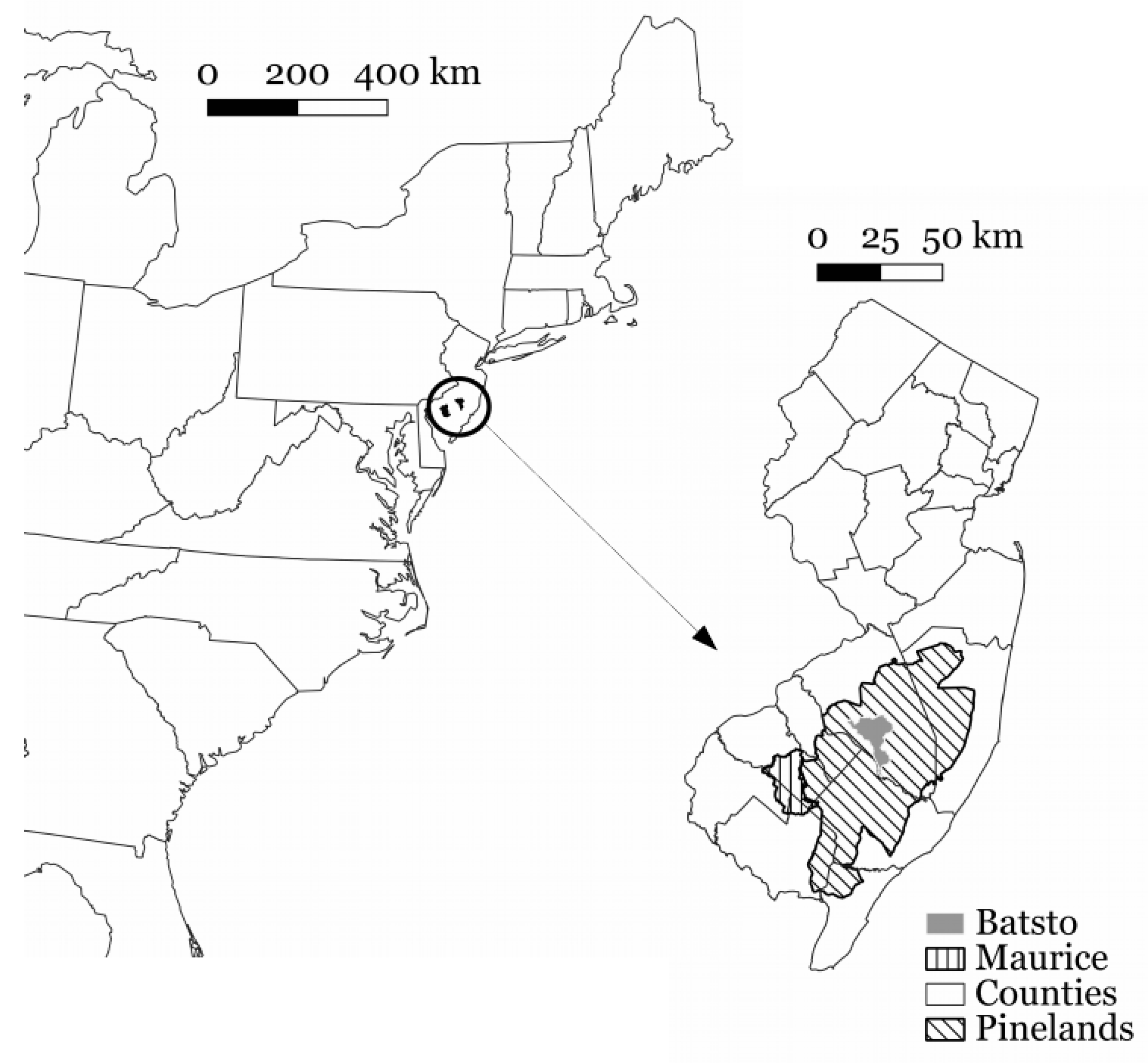
2.2. Site
2.3. Hydrologic Simulations and Bias Correction
2.3.1. Simulations Using Observed Data
2.3.2. Goodness-of-Fit
2.4. Simulations Using GCM Data
3. Results
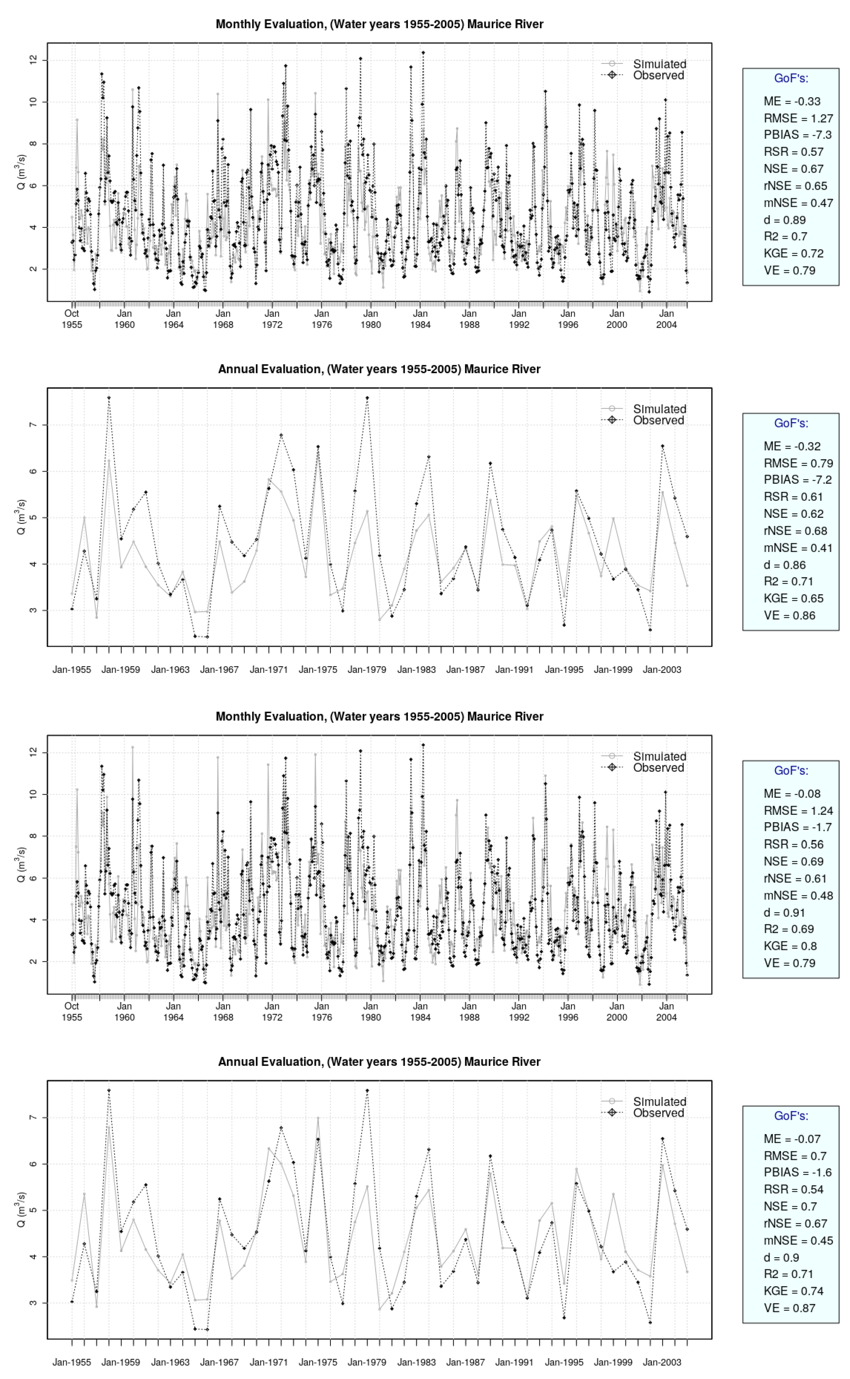
3.1. Simulations Driven by Observed Meteorological Data
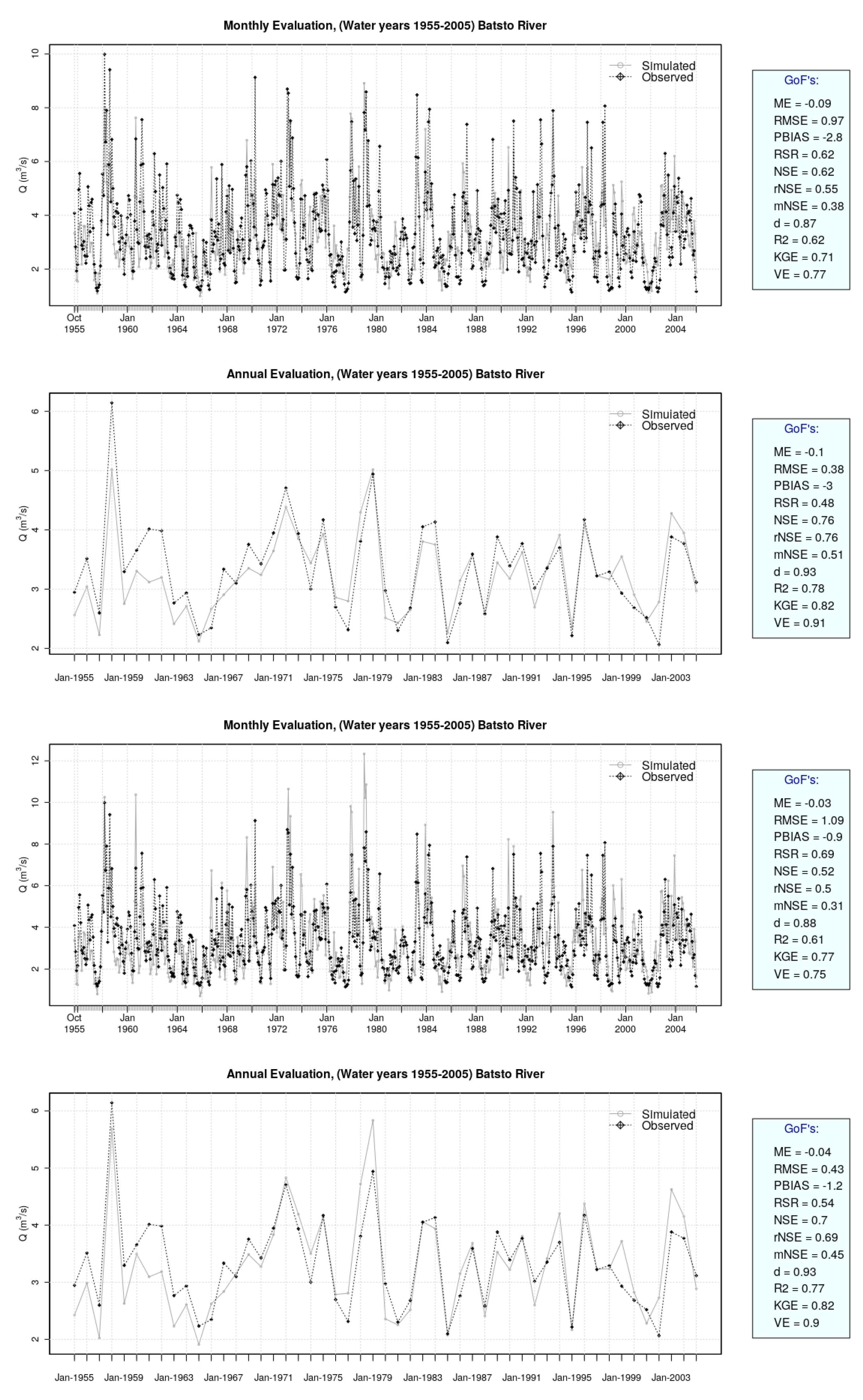
3.1.1. Goodness-of-Fit
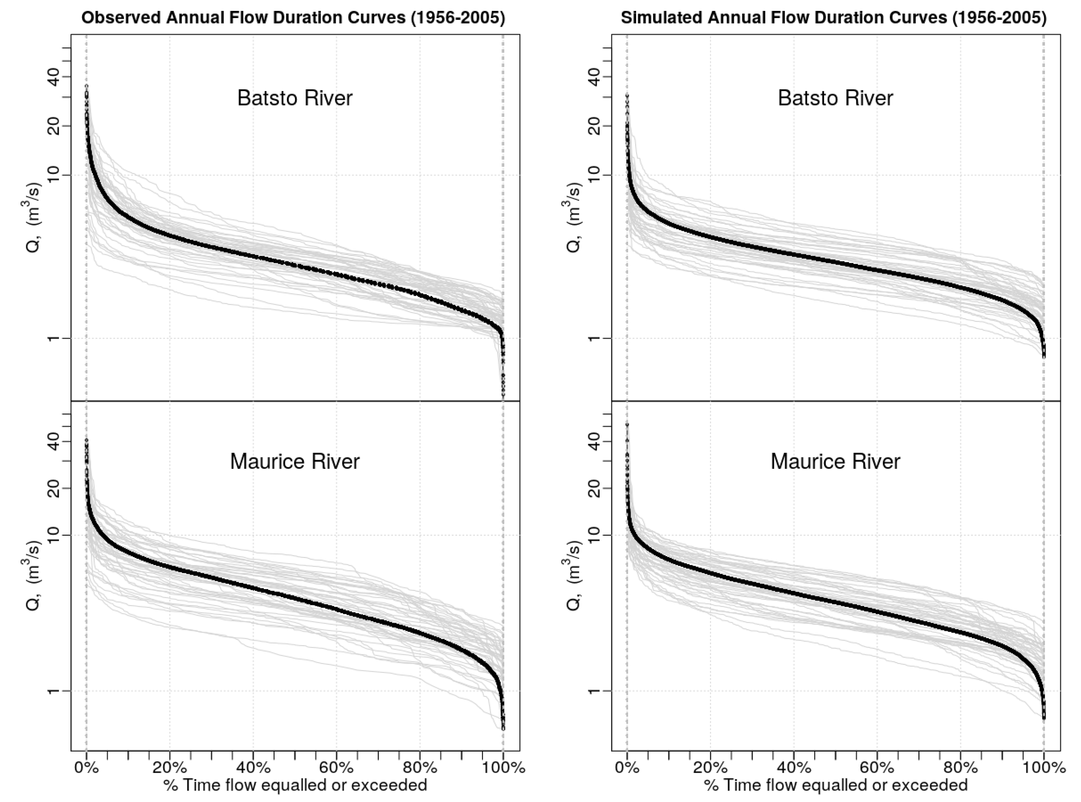
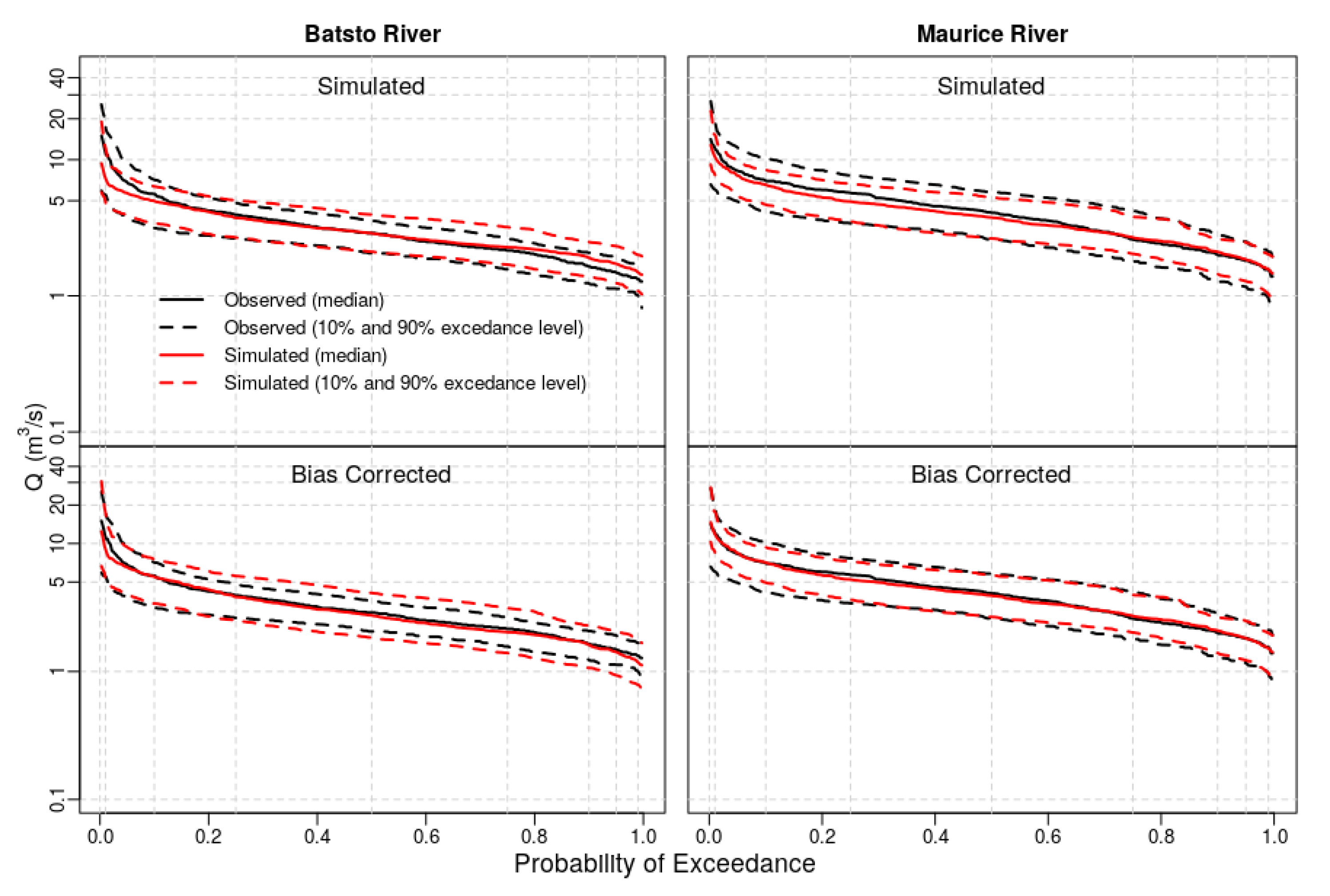
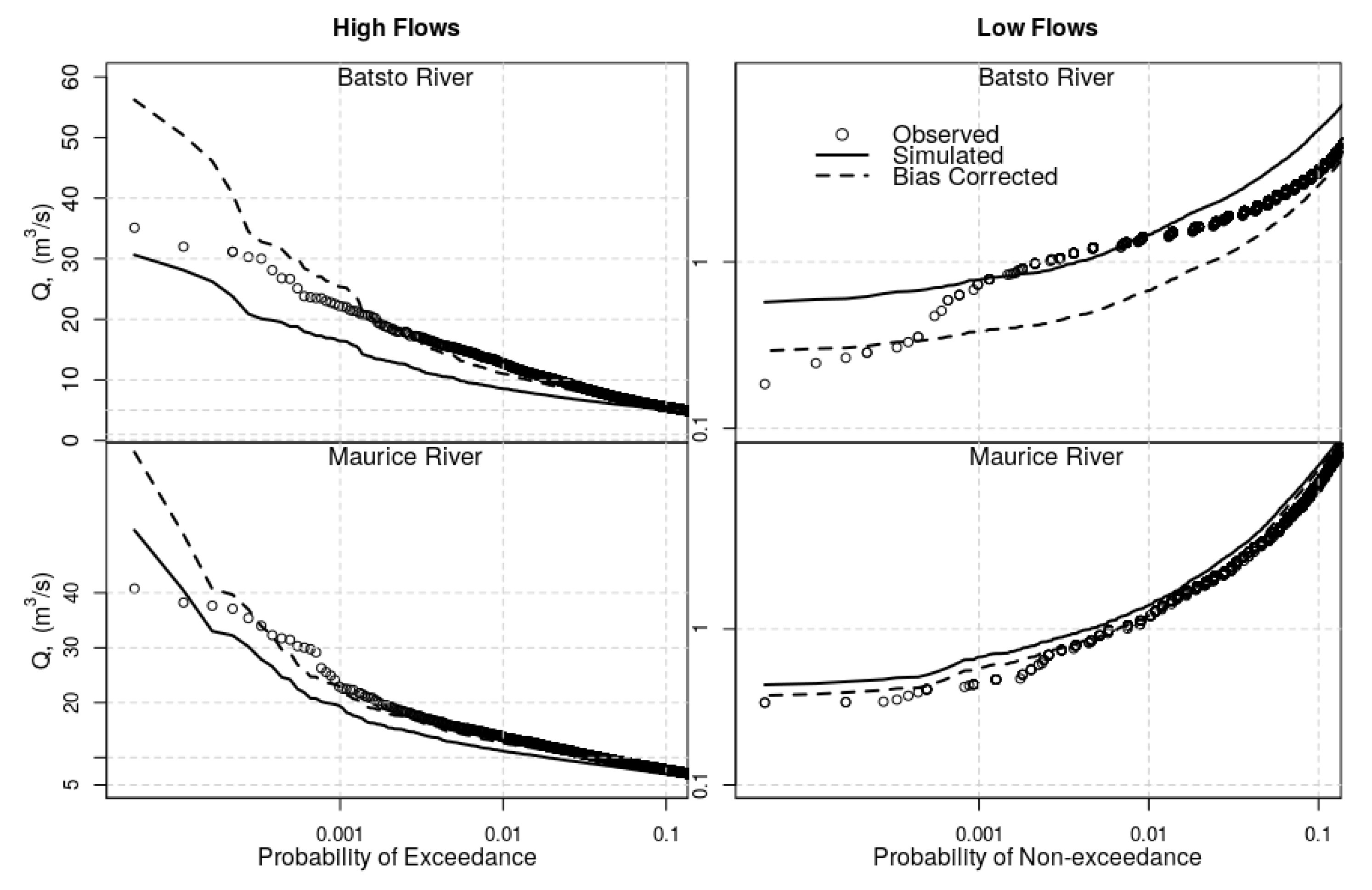
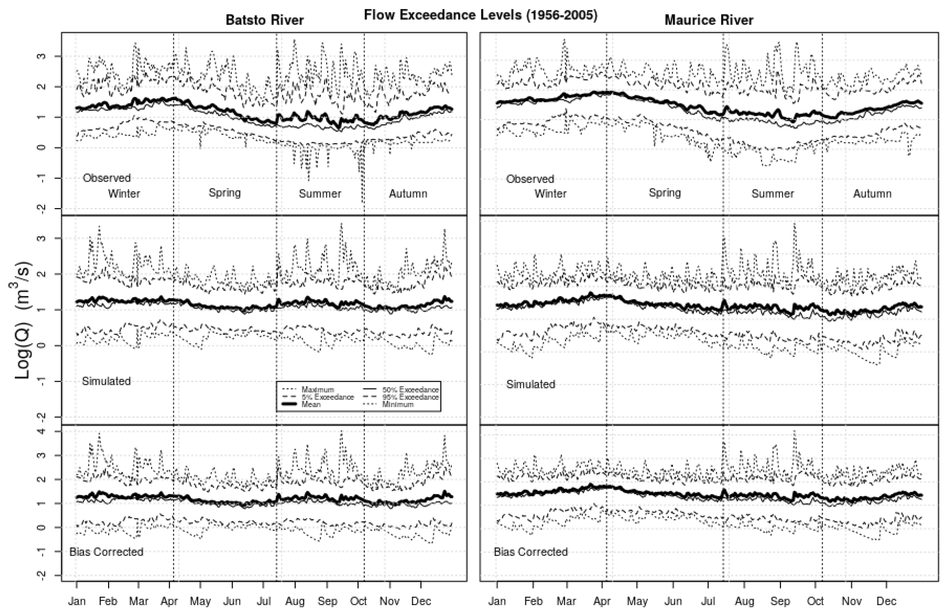
3.1.2. Flow Duration Curves
3.2. Simulations Using GCM Data
3.2.1. Historical Simulations
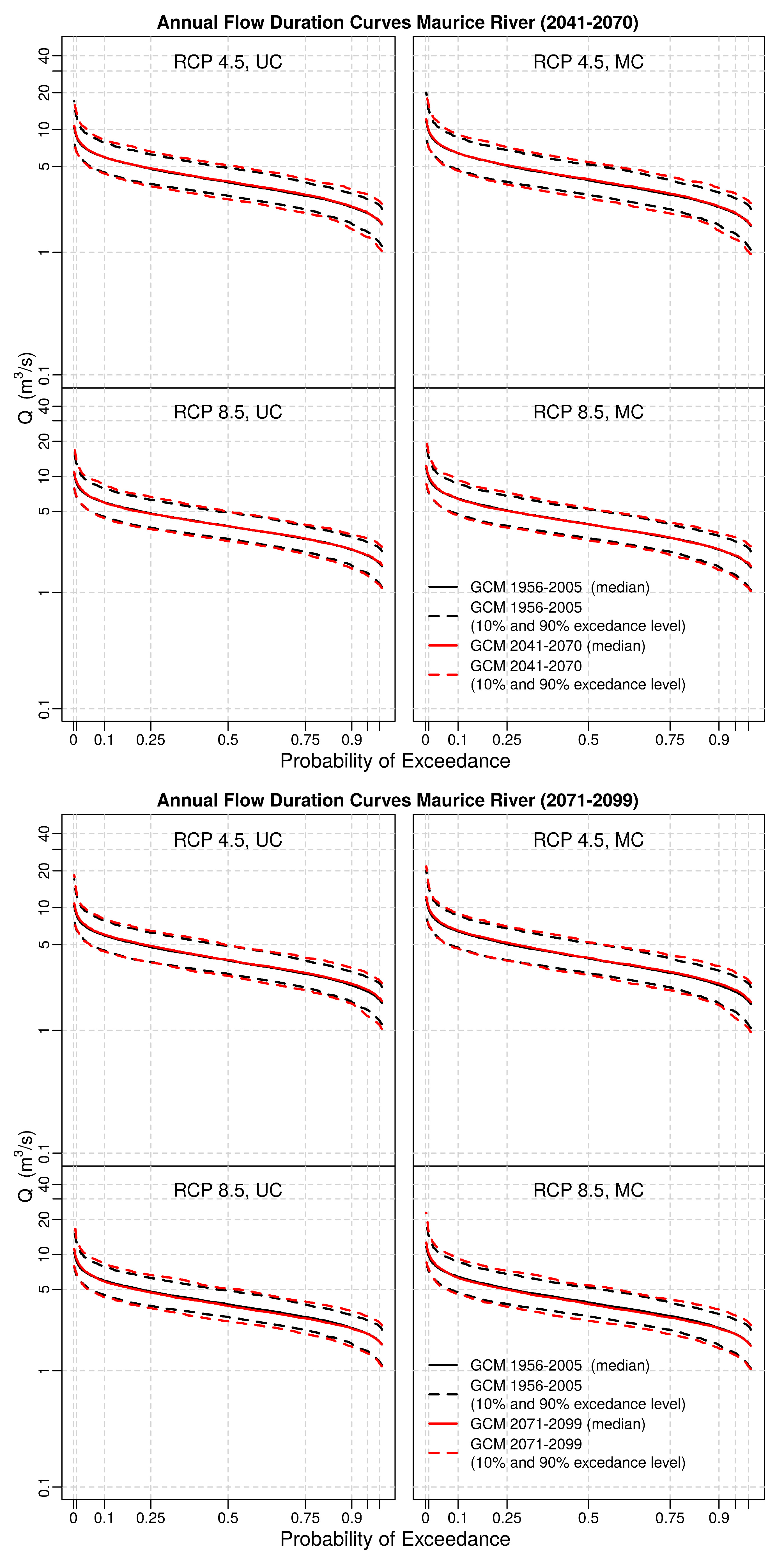
3.2.2. Projected Simulations
4. Discussion
4.1. Performance of the Hydrologic Model
4.2. Downscaled GCM-Driven Simulations
4.2.1. Bias Correction of Stream Flows
4.2.2. Climate Change Projections
Impacts of Watershed Characteristics
5. Conclusions
Funding
Acknowledgments
Conflicts of Interest
Abbreviations
| GCM | general circulation model |
| BCCA | bias correction with constructed analogs |
| FDC | flow duration curve |
| PRMS | precipitation-runoff modeling system |
| NJ | New Jersey |
| CMIP | Coupled Model Intercomparison Project |
| CDF | cumulative density function |
| UC | uncorrected |
| BC | bias corrected |
| MC | model corrected |
| GoF | goodness-of-fit |
References
- Westerberg, I.K.; Guerrero, J.L.; Younger, P.M.; Beven, K.J.; Seibert, J.; Halldin, S.; Freer, J.E.; Xu, C.Y. Calibration of hydrological models using flow-duration curves. Hydrol. Earth Syst. Sci. 2011, 15, 2205–2227. [Google Scholar] [CrossRef] [Green Version]
- Shamir, E.; Imam, B.; Morin, E.; Gupta, H.V.; Sorooshian, S. The role of hydrograph indices in parameter estimation of rainfall-runoff models. Hydrol. Process. 2005, 19, 2187–2207. [Google Scholar] [CrossRef] [Green Version]
- Gupta, H.V.; Sorooshian, S.; Yapo, P.O. Toward improved calibration of hydrologic models: Multiple and noncommensurable measures of information. Water Resour. Res. 1998, 34, 751–763. [Google Scholar] [CrossRef]
- Parada, L.M.; Fram, J.P.; Liang, X. Multi-Resolution Calibration Methodology for Hydrologic Models: Application to a Sub-Humid Catchment. In Calibration of Watershed Models; American Geophysical Union (AGU): Washington, DC, USA, 2013; pp. 197–211. [Google Scholar] [CrossRef]
- Vaze, J.; Post, D.; Chiew, F.; Perraud, J.M.; Viney, N.; Teng, J. Climate non-stationarity – Validity of calibrated rainfall–runoff models for use in climate change studies. J. Hydrol. 2010, 394, 447–457. [Google Scholar] [CrossRef]
- Kurkute, S.; Li, Z.; Li, Y.; Huo, F. Assessment and projection of the water budget over western Canada using convection-permitting weather research and forecasting simulations. Hydrol. Earth Syst. Sci. 2020, 24, 3677–3697. [Google Scholar] [CrossRef]
- Qing, Y.; Wang, S.; Zhang, B.; Wang, Y. Ultra-high resolution regional climate projections for assessing changes in hydrological extremes and underlying uncertainties. Clim. Dyn. 2020. [Google Scholar] [CrossRef]
- Chen, C.; Kalra, A.; Ahmad, S. Hydrologic responses to climate change using downscaled GCM data on a watershed scale. J. Water Clim. Chang. 2018, 10, 63–77. [Google Scholar] [CrossRef]
- Burgan, H.I.; Aksoy, H. Monthly Flow Duration Curve Model for Ungauged River Basins. Water 2020, 12, 338. [Google Scholar] [CrossRef] [Green Version]
- Chouaib, W.; Alila, Y.; Caldwell, P.V. On the use of mean monthly runoff to predict the flow–duration curve in ungauged catchments. Hydrol. Sci. J. 2019, 64, 1573–1587. [Google Scholar] [CrossRef]
- Hrachowitz, M.; Savenije, H.H.; Blöschl, G.; McDonnell, J.J.; Sivapalan, M.; Pomeroy, J.W.; Arheimer, B.; Blume, T.; Clark, M.P.; Ehret, U.; et al. A decade of Predictions in Ungauged Basins (PUB)-a review. Hydrol. Sci. J. 2013, 58, 1198–1255. [Google Scholar] [CrossRef]
- Troin, M.; Arsenault, R.; Martel, J.L.; Brissette, F. Uncertainty of Hydrological Model Components in Climate Change Studies over Two Nordic Quebec Catchments. J. Hydrometeorol. 2018, 19, 27–46. [Google Scholar] [CrossRef]
- Santos, C.A.; Almeida, C.; Ramos, T.B.; Rocha, F.A.; Oliveira, R.; Neves, R. Using a hierarchical approach to calibrate SWAT and predict the semi-arid hydrologic regime of northeastern Brazil. Water 2018, 10, 1137. [Google Scholar] [CrossRef]
- Kim, D.; Jung, I.W.; Chun, J.A. A comparative assessment of rainfall-runoff modeling against regional flow duration curves for ungauged catchments. Hydrol. Earth Syst. Sci. 2017, 21, 5647–5661. [Google Scholar] [CrossRef]
- Vogel, R.M.; Fennessey, N.M. Flow Duration Curves Ii: A Review of Applications in Water Resources Planning. Water Resour. Bull. Am. Water Resour. Assoc. 1995, 31, 1029–1039. [Google Scholar] [CrossRef]
- Muerth, M.J.; Gauvin St-Denis, B.; Ricard, S.; Velázquez, J.A.; Schmid, J.; Minville, M.; Caya, D.; Chaumont, D.; Ludwig, R.; Turcotte, R. On the need for bias correction in regional climate scenarios to assess climate change impacts on river runoff. Hydrol. Earth Syst. Sci. 2013, 17, 1189–1204. [Google Scholar] [CrossRef] [Green Version]
- Maraun, D.; Widmann, M. Statistical Downscaling and Bias Correction for Climate Research; Cambridge University Press: Cambridge, UK, 2018. [Google Scholar] [CrossRef] [Green Version]
- Daraio, J.A. Potential Climate Change Impacts on Streamflow and Recharge in Two Watersheds on the New Jersey Coastal Plain. J. Hydrol. Eng. 2017, 22, 05017002. [Google Scholar] [CrossRef]
- Leavesly, G.H.; Markstrom, S.L.; Viger, R.J. USGS Modular Modeling System (MMS)–Precipitation-Runoff Modeling System (PRMS). In Watershed Models; Singh, V.P., Frevert, D.K., Eds.; Taylor & Francis: Boca Raton, FL, USA, 2006; pp. 159–178. [Google Scholar]
- Hay, L.E.; Markstrom, S.L.; Ward-Garrison, C. Watershed-Scale Response to Climate Change through the Twenty-First Century for Selected Basins across the United States. Earth Interact. 2011, 15, 1–37. [Google Scholar] [CrossRef]
- Viger, R.J.; Hay, L.E.; Markstrom, S.L.; Jones, J.W.; Buell, G.R. Hydrologic Effects of Urbanization and Climate Change on the Flint River Basin, Georgia. Earth Interact. 2011, 15, 1–25. [Google Scholar] [CrossRef]
- Daraio, J.A.; Bales, J.D. Effects of Land Use and Climate Change on Stream Temperature I: Daily Flow and Stream Temperature Projections. JAWRA J. Am. Water Resour. Assoc. 2014, 50, 1155–1176. [Google Scholar] [CrossRef]
- Fahad, G.R.; Nazari, R.; Daraio, J.; Lundberg, D.J. Regional Study of Future Temperature and Precipitation Changes Using Bias Corrected Multi-Model Ensemble Projections Considering High Emission Pathways. J. Earth Sci. Clim. Chang. 2017, 8. [Google Scholar] [CrossRef]
- Krysanova, V.; Donnelly, C.; Gelfan, A.; Gerten, D.; Arheimer, B.; Hattermann, F.; Kundzewicz, Z.W. How the performance of hydrological models relates to credibility of projections under climate change. Hydrol. Sci. J. 2018, 63, 696–720. [Google Scholar] [CrossRef]
- Bourdin, D.R.; Stull, R.B. Bias-corrected short-range Member-to-Member ensemble forecasts of reservoir inflow. J. Hydrol. 2013, 502, 77–88. [Google Scholar] [CrossRef]
- Zalachori, I.; Ramos, M.H.; Garçon, R.; Mathevet, T.; Gailhard, J. Statistical processing of forecasts for hydrological ensemble prediction: A comparative study of different bias correction strategies. Adv. Sci. Res. 2012, 8, 135–141. [Google Scholar] [CrossRef] [Green Version]
- Pagano, T.C.; Wang, Q.J.; Hapuarachchi, P.; Robertson, D. A dual-pass error-correction technique for forecasting streamflow. J. Hydrol. 2011, 405, 367–381. [Google Scholar] [CrossRef]
- Hashino, T.; Bradley, A.A.; Schwartz, S.S. Evaluation of bias correction methods for ensemble streamflow volume forecasts. Hydrol. Earth Syst. Sci. 2007, 11, 939–950. [Google Scholar] [CrossRef] [Green Version]
- Li, Y.; Jiang, Y.; Lei, X.; Tian, F.; Duan, H.; Lu, H. Comparison of precipitation and streamflow correcting for ensemble streamflow forecasts. Water 2018, 10, 177. [Google Scholar] [CrossRef] [Green Version]
- Yuan, X.; Wood, E.F. Downscaling precipitation or bias-correcting streamflow? Some implications for coupled general circulation model (CGCM)-based ensemble seasonal hydrologic forecast. Water Resour. Res. 2012, 48, 1–7. [Google Scholar] [CrossRef]
- Beven, K.J. A manifesto for the equifinality thesis. J. Hydrol. 2006, 320, 18–36. [Google Scholar] [CrossRef] [Green Version]
- Delignette-Muller, M.L.; Dutang, C. Fitdistrplus: An R Package for Fitting Distributions. J. Stat. Softw. 2015, 64, 1–34. [Google Scholar] [CrossRef] [Green Version]
- R Core Team. R: A Language and Environment for Statistical Computing; R Foundation for Statistical Computing: Vienna, Austria, 2018. [Google Scholar]
- Gudmundsson, L.; Bremnes, J.B.; Haugen, J.E.; Engen-Skaugen, T. Technical Note: Downscaling RCM precipitation to the station scale using statistical transformations—A comparison of methods. Hydrol. Earth Syst. Sci. 2012, 16, 3383–3390. [Google Scholar] [CrossRef] [Green Version]
- Gudmundsson, L. Qmap: Statistical Transformations for Post-Processing Climate Model Output; R Package Version 1.0-4. 2016. Available online: https://cran.r-project.org/ (accessed on 18 August 2020).
- Zambrano-Bigiarini, M. hydroGOF: Goodness-of-Fit Functions for Comparison of Simulated and Observed Hydrological Time Series; R Package Version 0.3-10. 2017. Available online: https://cran.r-project.org/ (accessed on 18 August 2020).
- Maurer, E.P.; Wood, A.W.; Adam, J.C.; Lettenmaier, D.P.; Nijssen, B. A Long-Term Hydrologically-Based Data Set of Land Surface Fluxes and States for the Conterminous United States. J. Clim. 2002, 15, 3237–3251. [Google Scholar] [CrossRef] [Green Version]
- Taylor, K.E.; Stouffer, R.J.; Meehl, G.A. An Overview of CMIP5 and the Experiment Design. Bull. Am. Meteorol. Soc. 2012, 93, 485–498. [Google Scholar] [CrossRef] [Green Version]
- Brekke, L.; Wood, A.; Pruitt, T. Downscaled CMIP3 and CMIP5 Climate and Hydrology Projections: Release of Downscaled CMIP5 Climate Projections, Comparison with preceding Information, and Summary of User Needs. 2014. Available online: http://gdo-dcp.ucllnl.org/downscaled_cmip_projections/ (accessed on 10 August 2020).
- Bracken, C. Downscaled CMIP3 and CMIP5 Climate Projections—Addendum. 2016. Available online: https://gdo-dcp.ucllnl.org/downscaled_cmip_projections/techmemo/Downscaled_Climate_Projections_Addendum_Sept2016.pdf (accessed on 10 August 2020).
- Wang, S.; Wang, Y. Improving probabilistic hydroclimatic projections through high-resolution convection-permitting climate modeling and Markov chain Monte Carlo simulations. Clim. Dyn. 2019, 53, 1613–1636. [Google Scholar] [CrossRef]
- Beven, K.J. Preferential flows and travel time distributions: Defining adequate hypothesis tests for hydrological process models. Hydrol. Process. 2010, 24, 1537–1547. [Google Scholar] [CrossRef]
- Moriasi, D.N.; Gitau, M.W.; Pai, N.; Daggupati, P. Hydrologic and Water Quality Models: Performance Measures and Evaluation Criteria. Trans. ASABE 2015, 58, 1763–1785. [Google Scholar] [CrossRef] [Green Version]
- Ritter, A.; Muñoz-Carpena, R. Performance evaluation of hydrological models: Statistical significance for reducing subjectivity in goodness-of-fit assessments. J. Hydrol. 2013, 480, 33–45. [Google Scholar] [CrossRef]
- Legates, D.R.; McCabe, G.J. Evaluating the use of ’goodness-of-fit’ measures in hydrologic and hydroclimatic model validation. Water Resour. Res. 1999, 35, 233–241. [Google Scholar] [CrossRef]
- Gupta, H.V.; Kling, H.; Yilmaz, K.K.; Martinez, G.F. Decomposition of the mean squared error and NSE performance criteria: Implications for improving hydrological modeling. J. Hydrol. 2009, 377, 80–91. [Google Scholar] [CrossRef] [Green Version]
- Walker, R.L.; Nicholson, R.S.; Storck, D.A. Hydrologic Assessment of Three Drainage Basins in the Pinelands of Southern New Jersey, 2004-06; Technical Report 2011-5056; U.S. Geological Survey Scientific Investigations: Reston, VA, USA, 2011; 145p. [Google Scholar]
- Shi, X.; Wood, A.W.; Lettenmaier, D.P. How Essential is Hydrologic Model Calibration to Seasonal Streamflow Forecasting? J. Hydrometeorol. 2008, 9, 1350–1363. [Google Scholar] [CrossRef]
- Clark, M.P.; Wilby, R.L.; Gutmann, E.D.; Vano, J.A.; Gangopadhyay, S.; Wood, A.W.; Fowler, H.J.; Prudhomme, C.; Arnold, J.R.; Brekke, L.D. Characterizing Uncertainty of the Hydrologic Impacts of Climate Change. Curr. Clim. Chang. Rep. 2016, 2, 55–64. [Google Scholar] [CrossRef] [Green Version]
- Wilby, R.L.; Harris, I. A framework for assessing uncertainties in climate change impacts: Low-flow scenarios for the River Thames, UK. Water Resour. Res. 2006, 42. [Google Scholar] [CrossRef]
- Poff, N.L.; Allan, J.D.; Bain, M.B.; Karr, J.R.; Prestegaard, K.L.; Richter, B.D.; Sparks, R.E.; Stromberg, J.C. The Natural Flow Regime. BioScience 1997, 47, 769–784. [Google Scholar] [CrossRef]
- Euser, T.; Winsemius, H.C.; Hrachowitz, M.; Fenicia, F.; Uhlenbrook, S.; Savenije, H.H. A framework to assess the realism of model structures using hydrological signatures. Hydrol. Earth Syst. Sci. 2013, 17, 1893–1912. [Google Scholar] [CrossRef] [Green Version]
- Archfield, S.A.; Kennen, J.G.; Carlisle, D.M.; Wolock, D.M. An Objective and Parsimonious Approach for Classifying Natural Flow Regimes at a Continental Scale. River Res. Appl. 2014, 30, 1166–1183. [Google Scholar] [CrossRef]
- Poff, N.L.; Zimmerman, J.K. Ecological responses to altered flow regimes: A literature review to inform the science and management of environmental flows. Freshw. Biol. 2010, 55, 194–205. [Google Scholar] [CrossRef]


| Modeling Center (or Group) | Institute ID | Model Name |
|---|---|---|
| Commonwealth Scientific and Industrial Research Organization (CSIRO) and Bureau of Meteorology (BOM), Australia | CSIRO-BOM | ACCESS1.0 |
| Beijing Climate Center, China Meteorological Administration | BCC | BCC-CSM1.1 |
| College of Global Change and Earth System Science Beijing Normal University | GCESS | BNU-ESM |
| Canadian Centre for Climate Modelling and | CCCMA | CanESM2 |
| National Center for Atmospheric Research | NCAR | CCSM4 |
| Community Earth System Model Contributors | NSF-DOE-NCAR | CESM1(BGC) |
| Centre National de Recherches Météorologiques/Centre Européen de Recherche et Formation Avancée en Calcul Scientifique | CNRM-CERFACS | CNRM-CM5 |
| Commonwealth Scientific and Industrial Research Organization in collaboration with Queensland Climate Change Centre of Excellence | CSIRO-QCCCE | CSIRO-Mk3.6.0 |
| Institute for Numerical Mathematics | INM | INM-CM4 |
| Institut Pierre-Simon Laplace | IPSL | IPSL-CM5A-LR |
| IPSL-CM5A-MR | ||
| Japan Agency for Marine-Earth Science and Technology, Atmosphere and Ocean Research Institute (The University of Tokyo), and National Institute for Environmental Studies | MIROC | MIROC-ESM MIROC-ESM-CHEM |
| Atmosphere and Ocean Research Institute (The University of Tokyo), National Institute for Environmental Studies, and Japan Agency for Marine-Earth Science and Technology | MIROC | MIROC5 |
| Max-Planck-Institut für Meteorologie (Max Planck Institute for Meteorology) | MPI-M | MPI-ESM-MR MPI-ESM-LR |
| Meteorological Research Institute | MRI | MRI-CGCM3 |
| Norwegian Climate Centre | NCC | NorESM1-M |
| ME | Mean Error | |
| R2 | Coefficient of variation | |
| RMSE | Root Mean Squared Error | |
| PBIAS | Percent Bias | |
| NSE | Nash–Sutcliffe Efficiency | , |
| d | Index of agreement | , |
| KGE | Kling–Gupta Efficiency | |
| ; , | ||
| VE | Volumetric efficiency | , |
| UC | BC | |||||||
|---|---|---|---|---|---|---|---|---|
| Batsto River | ||||||||
| GoF | DJF | MAM | JJA | SON | DJF | MAM | JJA | SON |
| ME (m3s−1) | −0.71 | −0.32 | 0.74 | 0.04 | −0.54 | −0.36 | 0.85 | 0.06 |
| R2 | 0.57 | 0.61 | 0.65 | 0.63 | 0.56 | 0.63 | 0.66 | 0.61 |
| RMSE (m3s−1) | 1.69 | 1.41 | 1.61 | 1.11 | 1.86 | 1.32 | 1.74 | 1.34 |
| PBIAS% | −16.70 | −9.70 | 28.90 | 1.40 | −12.60 | −10.70 | 32.90 | 2.10 |
| NSE | 0.48 | 0.54 | 0.55 | 0.63 | 0.37 | 0.60 | 0.47 | 0.45 |
| d | 0.82 | 0.80 | 0.84 | 0.88 | 0.85 | 0.86 | 0.87 | 0.87 |
| KGE | 0.62 | 0.51 | 0.56 | 0.74 | 0.69 | 0.65 | 0.61 | 0.72 |
| VE | 0.74 | 0.76 | 0.57 | 0.78 | 0.70 | 0.75 | 0.57 | 0.74 |
| Maurice River | ||||||||
| ME (m3s−1) | −0.96 | −0.57 | 0.60 | −0.25 | −0.63 | −0.31 | 0.82 | −0.07 |
| R2 | 0.39 | 0.51 | 0.46 | 0.47 | 0.38 | 0.50 | 0.45 | 0.46 |
| RMSE (m3s−1) | 2.39 | 1.90 | 2.25 | 1.68 | 2.41 | 1.92 | 2.52 | 1.78 |
| PBIAS% | −16.70 | −11.60 | 18.50 | −6.40 | −11.00 | −6.30 | 25.20 | −1.70 |
| NSE | 0.21 | 0.45 | 0.36 | 0.40 | 0.20 | 0.44 | 0.20 | 0.33 |
| d | 0.75 | 0.81 | 0.80 | 0.82 | 0.77 | 0.83 | 0.79 | 0.82 |
| KGE | 0.56 | 0.63 | 0.62 | 0.67 | 0.59 | 0.69 | 0.58 | 0.68 |
| VE | 0.71 | 0.74 | 0.63 | 0.71 | 0.71 | 0.74 | 0.59 | 0.69 |
© 2020 by the author. Licensee MDPI, Basel, Switzerland. This article is an open access article distributed under the terms and conditions of the Creative Commons Attribution (CC BY) license (http://creativecommons.org/licenses/by/4.0/).
Share and Cite
Daraio, J.A. Hydrologic Model Evaluation and Assessment of Projected Climate Change Impacts Using Bias-Corrected Stream Flows. Water 2020, 12, 2312. https://doi.org/10.3390/w12082312
Daraio JA. Hydrologic Model Evaluation and Assessment of Projected Climate Change Impacts Using Bias-Corrected Stream Flows. Water. 2020; 12(8):2312. https://doi.org/10.3390/w12082312
Chicago/Turabian StyleDaraio, Joseph A. 2020. "Hydrologic Model Evaluation and Assessment of Projected Climate Change Impacts Using Bias-Corrected Stream Flows" Water 12, no. 8: 2312. https://doi.org/10.3390/w12082312
APA StyleDaraio, J. A. (2020). Hydrologic Model Evaluation and Assessment of Projected Climate Change Impacts Using Bias-Corrected Stream Flows. Water, 12(8), 2312. https://doi.org/10.3390/w12082312