Impact of Standing Column Well Operation on Carbonate Scaling

Abstract

Standing column well constitutes a recent promising solution to provide heating or cooling and to reduce greenhouse gases emissions in urban areas. Nevertheless, scaling issues can emerge in presence of carbonates and impact their efficiency. Even though a thermo-hydro-geochemical model demonstrated the impact of the water temperature on carbonate concentration, this conclusion has not been yet demonstrated by field investigations. To do so, an experimental ground source heat pump system connected to a standing column well was operated under various conditions to collect 50 groundwater samples over a period of 267 days. These field samples were used for mineral analysis and laboratory batch experiments. The results were analyzed with multivariate regression and geochemical simulations and confirmed a clear relationship between the calcium concentrations measured in the well, the temperature and the calcite equilibrium constant. It was also found that operating a ground source heat pump system in conjunction with a small groundwater treatment system allows reduction of calcium concentration in the well, while shutting down the system leads to a quite rapid increase at a level consistent with the regional calcium concentration. Although no major clogging or biofouling problem was observed after two years of operation, mineral scales made of carbonates precipitated on a flowmeter and hindered its operation. The paper provides insight on the impact of standing column well on groundwater quality and suggests some mitigation measures.

1. Introduction

Nowadays, it is mostly accepted that greenhouse gases are responsible for global warming [1]. Ground source heat pumps (GSHPs) have the capacity to reduce greenhouse gas emissions for heating and cooling buildings [2], which represented 61% of the total energy consumption in the commercial and institutional sector in Canada in 2016 [3]. The GSHPs are sustainable technologies [4]. Due to their renewable aspect and mostly their high energy efficiency, the number of GSHPs has been rising worldwide over the past 15 years [5]. Among the different types of ground heat exchangers, standing column wells (SCWs) have proven to be a promising solution because of their high heat exchange rate and lower first costs [6,7]. Another significant advantage is that SCWs can be installed more easily in urban areas as they require a smaller footprint than closed-loop systems, and less groundwater than open-loop systems [8].

Basically, an SCW is a coaxial uncased well (see Figure 1), in which the groundwater is continuously recirculated. This brings the groundwater into direct contact with the surrounding rock and allows heat transfer by conduction along the borehole wall [6,8]. During peak periods, part of the circulation flow rate is discharged outside the SCW. This process creates a cone of depression around the SCW and induces a convergent groundwater flow, increasing advective heat transfer that enhances the thermal performances of the SCW [8,9]. However, since the groundwater is directly used as the heat carrier fluid, clogging processes can affect the SCW [10] and the various mechanical devices [11] connected to it.

Indeed, precipitation can increase resistance to groundwater flow inside the pipes, obstruct the heat exchanger and the submersible pump. The latter can increase pump fatigue, which could lead to its premature failure [11]. Besides, precipitation within the heat exchanger can also reduce the energy supplied to the GSHPs [11,12] and lead to a lower coefficient of performance. For instance, a deposit of 0.8 mm on a heat exchanger surface can increase the GSHP consumption by 19% [13]. Several elements are indicators of active clogging processes within GSHP systems. These processes can have a physical [14,15], microbiological [10,16,17] or chemical [18,19,20] source. However, in most cases clogging appears by a combination of more than one of those sources [21,22].

Many factors can promote clogging processes in carbonate environments. Indeed, the higher partial pressure of carbon dioxide in groundwater with respect to the atmosphere promotes $C{O}_2$ degassing, which in turn increases calcite nucleation and precipitation. In a system using groundwater as the heat carrier fluid, these processes are active at the free surface since pumping operations induce a water level variation [23] and a turbulent flow inside the well [20]. The same processes are also active in the injection well [24] or in the hydraulic circuit if zones of low pressure are present [25]. The dynamic operation of a system has also an impact on water quality. For instance, at system startup, the particle load increases in the well [15] while stagnant conditions occurring during downtime phases promote oxygenation, that in turn favors microbial abundance and diversity in the well [26].

The operation of a GSHP modifies the groundwater temperature (hotter during cooling mode, cooler during heating mode). Recently, the operation of a SCW has been simulated with a coupled thermo-hydro-geochemical model [8,27,28]. These works clearly showed that during heating mode, the continuous recirculation of cold groundwater in a SCW promotes calcite dissolution and enrichment of $C{a}^{2+}$. On the opposite, it was observed numerically that the cooling mode promotes precipitation mostly in the above-ground equipment. This advanced model was further exploited and revealed that sealing the SCW to prevent $C{O}_2$ degassing decreased by 33.3% the precipitation rate of calcite [28], and that a constant bleed rate of 10% reduced the calcite accumulation on borehole walls due to smaller temperature variations in the SCW [27].

The previous numerical results were obtained considering the equilibrium reactions and kinetics of calcite [29]. However, for the operating temperatures of a GSHP, laboratory tests indicated that calcite precipitation is inhibited by the presence in groundwater of orthophosphates [30], magnesium and organic acids [31,32]. Thus, simple geochemical models cannot be used alone to predict calcite precipitation in natural systems and should be complemented by field investigations. Study of biofouling occurring in an SCW has already been study for hydrous ferric oxides [10,33]. However, even though calcium carbonates are the most common scale deposit in open-loop residential systems [34], carbonates precipitation has yet not been studied during the operation of real SCW systems. This work aims to fulfill this gap of knowledge by using an GSHP system connected to an experimental SCW operated during 267 days under various cooling and heating conditions.

2. Site Description

The groundwater samples used to perform this study were collected through the use of a mobile geothermal laboratory that operates a SCW on a large scale. The following section presents the main components of this laboratory, the geochemical composition of the geological units crossed by the boreholes and the chemistry of the groundwater prior to the operation of the laboratory.

2.1. Geothermal Mobile Laboratory

The geothermal mobile laboratory (see Figure 1) is located in the city of Varennes, near Montreal in Canada. This infrastructure was designed to acquire information on the thermo-hydro-geochemical processes occurring during the operation of any ground heat exchanger such as open-loop, closed-loop or SCW [35,36]. The laboratory is composed of four water-to-air heat pumps of a total capacity of 56 kW. This allows emulation of the cooling and heating loads of a small building. To prevent clogging in the GSHPs, a plate heat exchanger separates the groundwater loop from a propylene glycol loop that supplies the GSHPs. All the equipment is held in a marine container to easily move it to different sites, as shown in Figure 2a and

Table 1. Equipment installed in the mobile geothermal laboratory.

Component	Manufacturer	Model	Main Characteristics
Four heat pump	Trane	DXVF04817	Net cooling capacity 48.81 MBh
Heat exchanger	Mueller	LC-150 53	hours capacity 244 117 BTU/h
Submersible pump	Goulds water technology	65GS50	Flow range 30–80 GPM

.

As shown in Figure 1, the groundwater loop includes a submersible pump, two flowmeters (F-GW and F-Bleed), two temperature sensors ($EWT$ and $LWT$) and four sample points (SP-1 to SP-4). The recording equipment and its accuracy are presented in

Table 2. Accuracy of the sensors installed in the mobile geothermal laboratory, from [36].

Component	Manufacturer	Model	Accuracy
Energy valve	Belimo	AKRB24-EV	±2%
Electromagnetic flowmeter	Endress + Hauser	Proline Promag 53	±0.2%
Temperature sensor	Greystone	TE200	±0.2 °C
Optical fiber	Sensornet		±1 °C

. Note that a groundwater treatment unit is also installed just before the plate heat exchanger to reduce clogging and scaling in the various parts of the system. Initially, the goal was to divert 20% of the groundwater to the treatment unit withdrawn by the submersible pump. Due to higher head loss than expected, only 3% to 7% of the total flow rate is actually treated. Since the groundwater is continually recirculated in the SCW, this allows treating all the groundwater of the SCW after a few cycles. The unit is composed of a sediment filter and two water softeners to protect the cation-ion exchange resin, which is regenerated with a brine. A disinfection system completes the groundwater treatment unit. The disinfection system is composed of one micro-filter, two low capacity ozone generators and one UV lamp. The characteristics of these devices are presented in

Table 3. Equipment of the groundwater treatment unit.

Component	Manufacturer	Model	Main Characteristics
Sediment filter	JUDO PROFI	JPF-ATP 1$\raisebox{1ex}{$1$}\!\left/ \!\raisebox{-1ex}{$2$}\right.$	Ø = 0.1 mm
Water softener	Advanced Water Products	AWPBFI-1044AN	nominal flow = 18.93 L/min
Cation exchange resin	Sanitizer	AWP1054SE2	nominal flow = 30.28 L/min
Micro-filter	VIQUA	AWP-40C-V	Ø = 5 $\mathsf{\mu }$m, nominal diameter
Ozone generator	VIQUA	S2Q-OZ	70 mg/h $O_3$ at 5 SCFH air flow
UV generator	TrojanUV	Pro10	40 mJ/cm${}^2$

and shown in Figure 2b. Thus, sample point 1 (SP-1) is used to collect groundwater at the outlet of the SCW. Sample point 2 (SP-2) allows collection of the treated water while sample point 3 (SP-3) collects the mix of treated water and groundwater just before the plate heat exchanger. After heat transfer occurs at the plate heat exchanger, the water is reinjected into the aquifer, either by the SCW or injection well. The reinjected water is sampled from the sample point 4 (SP-4).

2.2. Geology and Geochemistry

The GSHP system located in the laboratory is connected to a 300 m deep SCW (Ø 165 mm) and to a 150 m deep injection well (Ø 165 mm) located at a distance of 10 m. However, due to a delay to install the various pipes in the SCW, the bottom walls collapsed, resulting in an effective depth of 215 m. Notice that the SCW and injection well are not sealed and can therefore exchange gases with the atmosphere. A stratigraphic column of the geologic materials observed during drilling was established by Beaudry et al. [35,36] from the macroscopic observation of 54 samples taken every 6.1 m (see Figure 3). This analysis indicated the presence of an overburden composed of clayed silt from the surface to a depth of 3.1 m. For depths of 3.1 to 239.3 m, the bedrock is composed mainly of gray mudstone intersected locally by beds of siltstone, beige-pink sandstone, beige limestone and igneous rocks. This material is attributed to the Nicolet Formation of the Lorraine Group [37]. For the depths of 239.3 m to 305.3 m, a black shale limestone attributed to the Utica Group [37] was observed.

Due to the impact of the geology on groundwater quality, a geochemical analysis of the bedrock was performed on three composite rock samples taken randomly along the borehole (see Figure 3). To analyze each sample, the lithium tetraborate fusion method was used to determine the percentage of $Si{O}_2$, $A{l}_2{O}_3$, $CaO$, $MgO$, $FeO$, $N{a}_{2}O$, $K_{2}O$, $MnO$. A LECO CS-744 analyzer set at 1200 °C, was used to measure the concentration of S and of total carbon by infared spectrophotometry method. The $C{O}_2$ was determined by subtracting the total carbon to the carbon provided by the LECO CS-744 after a hydrochloric acid treatment (HCl at 50%) during 1 hour, according to the norm MA. 310-CS 1.0 [38]. The Loss On Ignition ($LOI$) was set at 1000 °C. An average was calculated from all the samples and results are presented in Figure 3 (right).

The results of the geochemical analyses indicated that the bedrock was mainly composed of silicates, with high concentrations of aluminum, calcium, magnesium and iron oxides. A significant concentration of sulfur was also observed. The percentage of calcium carbonate ($CaC{O}_3$) in the bedrock is calculated according to Equation (1) [39].

$$CaC{O}_3=M_{CaC{O}_3}/M_{CaO}·[CaO-(0.0448·A{l}_2{O}_3-0.001147)]$$

(1)

where $M_{CaC{O}_3}$, $M_{Ca}$ are the molar mass. The resulting fraction of calcium carbonate in the samples is 12.78%. Note the Equation (1) is initially developed for Netherlands geology. The calcium carbonate percentage indicates that the bedrock is chemically reactive with the groundwater circulating in the SCW or within the fractures [40]. It should be noted that a part of the calcium observed in the samples can be present in the form of calcium sulfates ($CaS{O}_4$), such as gypsum. In addition, due to the high percentage of magnesium oxides and $C{O}_2$, magnesium carbonate or dolomite ($CaMg{(C{O}_3)}_2$) can also be present in the sample.

2.3. Initial Chemical Composition of Groundwater

An initial sampling of the groundwater present in the SCW was performed on 11 November 2016. The results obtained are shown in

Table 4. Initial groundwater quality within the experimental SCW on 11 November 2016.

Parameter	Value	Unit
Calcium	32.40	ppm
Magnesium	13.00	ppm
Total hardness	134.0	ppm $CaC{O}_3$
Sulphate	90.60	ppm
Iron	0.34	ppm
Manganese	0.03	ppm
Total organic carbon	1.18	ppm
Inorganic carbon	83.70	ppm
Total Carbon	84.90	ppm
Sodium	310.00	ppm
Potassium	5.21	ppm
Bromide	1.20	ppm
Chloride	323.00	ppm
Fluoride	2.16	ppm
Ortho-phosphate	<0.05	ppm P
Nitrite	<0.10	ppm N
Nitrate	<0.10	ppm N
Total Alkalinity	370	ppm $CaC{O}_3$
pH	8.1
Conductivity	1870	$\mathsf{\mu }$S/cm
Temperature	11	°C

and indicated a total hardness of 134 ppm $CaC{O}_3$ and a pH of 8.1. These two values were above the values of 80 ppm and 7 recommended to avoid carbonate precipitation in GSHP systems [13]. Thus, carbonate scaling was expected to occur in various parts of the system. Note that it was not possible to perform more that one sampling before starting the operations of the laboratory and thus characterize the seasonal fluctuations of the groundwater chemistry.

3. Material and Method

First of all, this section presents the experience performed on the SCW. The groundwater samples were collected between January 2018 and October 2018 on a weekly basis (50 samples) under various conditions. These conditions are presented. A mineral scale sampled in January 2019 is presented. This sampling procedure and analysis method are presented. To interpret the groundwater calcium concentration during this operation, batch experiments of bedrock dissolution were performed in Polytechnique Montréal. The setup of batch experiments and the analysis method are presenting in this section. Finally, The chemical equations and software PHREEQC to calculated the kinetics and equilibrium for the batch experiments and the on-off sequence are presented.

3.1. Field Sampling and Groundwater Analysis

The test conditions were decomposed into five identifiable sequences. The first one was a heating mode, composed of demand peaks during the day. The second one was an On-Off sequence. The third one was composed of constant heating demand during the day. The fourth one was a period of cooling and recirculating, and the last sequence was a cooling mode. These conditions are summarized in

Table 5. Summary of test condition.

Name	Characteristics	Date
Heating-1	Heating period with cyclic loading of the heat demand	1st January to 20th February
On-Off sequence	10 involuntary On-Off operation	21st February to 26th March
Heating-2	Heating phase without cyclic demand during the day	27th March to 15th May
Cooling-Recirculating	Multiple operation	16th May to 27th Julyh
Cooling	Cooling with cyclic demand	28th July to 10th October

.

To collect representative groundwater samples, the following experimental protocol was established and upheld. Samples were collected after the submersible pump had been running for at least 5 min (even if a system downtime occurred during the previous days). Three flushes were performed for each sample point (SP-1 to SP-4) to eliminate any dead volume [41] before sampling. The measurements of temperature, pH, electrical conductivity and oxidation-reduction potential were then carried out with a multiparameter probe (YSI Pro Plus and Pro Series). The water was filtered with a 0.45 $\mathsf{\mu }$m hydrophilic polyvinylidene fluoride membrane (Millex-HV of Millipore). The samples dedicated to the analysis of iron and manganese were immediately acidified with a solution of $HN{O}_3$ having a pH lower than 2. All samples were stored at 4 °C for preservation until they were analyzed.

Analysis of the total soluble concentrations of $Fe$, $Mn$, $Ca$ and $Mg$ was carried out by atomic absorption with an Analyst 200 Spectrometer. The concentrations of major anions $F^{-}$, $C{l}^{-}$, $N{O}_2^{-}$, $B{r}^{-}$, $N{O}_3^{-}$, $S{O}_4^{2-}$, $P{O}_4^{3-}$ were determined by ionic chromatography with a Dionex ICS-5000 system. The detection limits of these two analysers were respectively 0.02 mg/L and 0.5 mg/L. A potentiometric titrator HI 901 measured the alkalinity.

3.2. Collection and Analysis of Mineral Scales

Installed in 2016, the flow meter F-GW began to malfunction between 10 October 2018 and 3 January 2019, until eventually it was decided to be disassembled. Observation of the flow meter piping indicated that mineral scales 0.8 mm thick were covering the inner piping (see Figure 4). The scales were tested with nitric acid (pH < 2) and reacted proving the presence of carbonates. Some mineral chips were then collected and stored in tubes for 2 days before a microscopic analysis was performed at the Centre for Characterization and Microscopy of Materials in Polytechnique Montréal. The analysis was carried out using three different technologies: a scanning electron microscope (SEM), an energy dispersive spectroscopy (EDS) and an X-ray diffraction. It is worth noting that no other major problems associated to scaling or biofouling were observed so far.

3.3. Batch Experiments

A batch experiment was designed to study the calcium equilibrium and dissolution kinetics of the rock samples gathered during the drilling of the experimental wells. To that end, rock samples with grain sizes between 1.25 mm and 0.63 mm (mean 0.66 mm) were selected. The samples were washed with demineralized water, followed by a bath of hydrochloric acid (0.012N) of 10 s to remove all impurities that were fixed to the surface during the drilling process [29]. Finally, the samples were rinsed with demineralized water to stop the reaction with hydrochloric acid. The rock samples were then dried at 65 °C to prevent burning any organic matter. The samples relative density was measured at 2.76 following the standard ASTM C128-15 [42]. Samples with a surface of approximately 8.25 cm${}^2$ were immerged in 80 mL of demineralized water (manufacture by Mili-DI) at 11 °C in microbiological bottles, as shown in Figure 5. The microbiological bottles were sealed with rubber bushings to perform the dissolution in a closed system. Trapped air was replaced by injecting nitrogen $N_2$. An orbital shaker then was used to stir the rock samples and the demineralized water together, without opening the solution to the atmosphere. Previous works indicated the rate of rotation has a pronounced impact at low pH (<5) while at higher pH the grain surface has the largest influence [29]. For this reason, the stirring speed was set to 200 rpm, speed at which the grain was suspended in the solution without mechanical shocks resulting of the impact with the microbiological bottles. During the batch experiment, the concentration of calcium and manganese was measured twice per day during one week by atomic absorption.

3.4. Geochemical Simulation

The simulation software PHREEQC [43] was used to perform two geochemical simulations. These simulations were used to analyze the dissolution kinetics and equilibrium of the batch experiments and the impact of GSHP downtimes on calcium concentration. The third simulation allowed computation of the saturation index ($SI$) of calcite in groundwater. The thermodynamic database WATEQ4F was adopted because it accounts for partial carbon dioxide pressure $P_{C{O}_2}$ and includes temperature of the solution [43]. This database has been used in related past studies [18,24] for these specific reasons. To simulate the dissolution kinetics of carbonate rock samples, PHREEQC uses the temperature dependent kinetics constants of calcite as identified by Plummer et al. [29].

To interpret the equilibrium of a mineral, PHREEQC calculates the saturation index in water by [40]:

$$SI=log\frac{IAP}{K(T)}$$

(2)

where $IAP$ represents the ionic activity product calculated from the activities of free ion species. In Equation (2), $K(T)$ is the temperature dependent equilibrium constant, with the temperature T in Kelvin. For a SI = 0 the mineral is at equilibrium; for SI < 0 the mineral is undersaturated, leading to a dominant dissolution state and if SI > 0 the mineral is oversaturated, leading to the precipitation of the mineral [40].

In this work, two temperature dependent equilibrium constants were used. The first equilibrium constant was for pure calcite and has been proposed by Plummer and Busenberg [44]:

$$log(K_{Calcite})=-171.9065-0.077993·T+\frac{2839.319}{T}+71.595·log(T)$$

(3)

An important feature of Equation (3) is that equilibrium constant decreases with temperature, leading to precipitation increase and calcium concentration reduction.

The second equilibrium constant considered the fact that magnesium inhibits calcite precipitation and that magnesian calcite ($C{a}_{1-x}M{g}_{x}C{O}_3$) is more stable than pure calcite. To model this situation, the concept of stoichiometric saturation proposed by Thorstenson and Plummer [45] was used. The dissolution reaction for magnesian calcite is then:

$$C{a}_{1-x}M{g}_{x}C{O}_3\stackrel{}{\to }(1-x)C{a}^{2+}·xM{g}^{2+}·C{O}_3^{2-}$$

(4)

where x is the molar concentration ratio between $\left[M{g}^{2+}\right]/\left[C{a}^{2+}\right]$ in the aqueous and solid solution. The equilibrium constant for magnesian calcite is:

$$K_{Mg-Calcite}=a_{C{a}^{2+}}^{(1-x)}·a_{M{g}^{2+}}^x·a_{C{O}_3^{2-}}$$

(5)

where $K_{Mg-Calcite}$ is the equilibrium constant, $a_{C{a}^{2+}}$, $a_{M{g}^{2+}}$ and $a_{C{O}_3^{2-}}$ are the activity of species in aqueous solution. The right side of Equation (5) is the $IAP$ used in Equation (2). The activities were calculated by PHREEQC using the final concentrations measured in the batch experiments described previously. At the end of dissolution, an equilibrium state was considered reached. The same kinetics of pure calcite developed by Plummer et al. [29] were used.

4. Results and Discussion

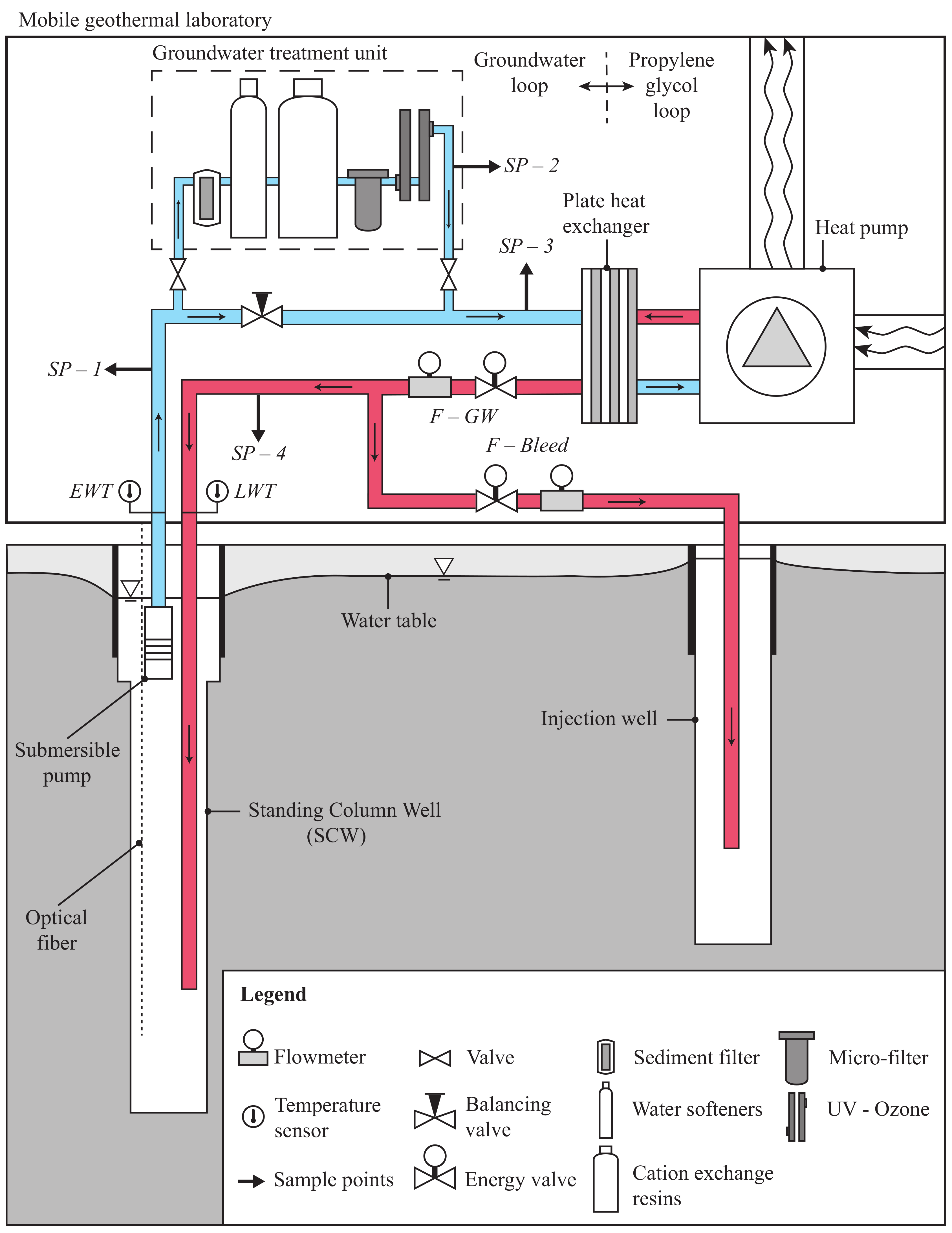
To identify the factors impacting carbonate scaling in a SCW, the geothermal laboratory and its groundwater treatment system were used between 16 January and 10 October 2018 under various heating and cooling conditions. During this period, the on-board data acquisition system recorded the operation parameters every minute, while groundwater sampling were performed on a weekly basis.

4.1. Geochemical Mapping

The analysis results of the samples collected at sample points 1 to 4 are presented in Figure 6. To compare the results coming from a large data set, whisker boxplots were used. The latter present the median, the 25% and 75% percentiles, as well as the minimum, maximum and outliers’ values. To observe the impact of the temperature on the water chemistry, the results were separated into two sets for each sample point based on the temperature measured at SP-1 during the groundwater sampling. The first set, shown in blue, is associated to temperatures equal to or lower than the initial groundwater temperature of 11 °C. The second set, shown in red, is associated to higher temperatures. This separation allowed us to study the impact of the cooling and heating mode.

The temperature at the sample points is shown in Figure 6a. Note that the number of samples n were uniformly distributed between the two sets of temperatures. The temperatures ranged between 1.3 °C at SP-4 and 36.2 °C at SP-1, and covered the typical temperatures observed during the operation of a SCW system in heating and cooling mode. The median temperatures were almost the same for a given set. However, the median temperature at the outlet of the plate heat exchanger (SP-4) was 2.3 °C, which was significantly lower than the other medians for the cold dataset. This difference is due to the heat extraction at the plate heat exchanger occurring in heating mode, confirming the separation as being representative of the heating mode.

As shown in Figure 6b, it is clear that the pH evolved as a function of the temperature since the pH was 0.3 units higher in heating mode than in cooling mode. The same pattern was also observed for the calcium and magnesium concentrations shown in Figure 6c,d. Indeed, the median concentrations were systematically lower at higher temperatures, which indicates that calcite precipitation probably occurred when the GSHP system was in cooling mode. These experimental observations are consistent with the results of Eppner et al. [27,28] who used a coupled geochemical model and observed numerically that recirculation of cold groundwater in a SCW promotes calcite dissolution and calcium enrichment, while recirculation of warmer groundwater during cooling mode favors calcite precipitation and calcium depletion. The fact that magnesium concentrations were also lower in cooling mode is a good indicator that dissolution and precipitation of dolomite or magnesian calcite were also active in the GSHP system. This is supported by the energy-dispersive spectroscopy test and the X-ray diffraction test carried out on the mineral scales shown in Figure 4. Indeed, the microscopic analysis pointed out mostly calcite and some magnesian calcite in the scales, confirming that precipitation processes were active.

The effect of the groundwater treatment system was clearly visible on the pH and on the calcium and magnesium concentrations coming from SP-2. Indeed, the median calcium concentration of the two temperature sets dropped by 80.8% and 88.9% at SP-2 with respect to SP-1. A similar result was observed with the magnesium, which dropped by 88.4% and 83.4%. These significant concentration reductions were partly attributed to the cation exchange resin and water softener installed in the groundwater treatment unit. The percentage of groundwater treated being small (3% to 7%), the impact of the treatment system on the concentrations measured at SP-3 and SP-4 was however smaller.

Nevertheless, the median concentrations of calcium and magnesium were significantly below their initial concentrations of 32.4 and 13.0 ppm, indicating that some processes were actively removing calcium from the groundwater. Based on the concentrations measured at the outlet of the groundwater treatment system (SP-2), it is clear that the continuous operation of the treatment unit could explain at least a part of these reductions. A second explanation lies in the probable impact of temperature on the equilibrium constants, which induces calcite precipitation and pH drop when the SCW is operated in cooling mode [27,28]. Degassing of $C{O}_2$ can also explain a part of the calcium reduction [28]. Based on these sole results, it is however impossible to distinguish which process controls mostly precipitation.

4.2. Impact of Temperature and GSHP Operation

It was shown in Section 4.1 that groundwater temperatures can impact calcium concentrations at a detectable level. However, this analysis did not allow to identify the impact of more complex GSHP operations. One can now see in Figure 7 the temporal evolution of calcium concentration, temperature and flow rate for various GSHP operation modes. First, note how calcium concentrations varied in time as a function of the GSHP operation mode in a quite complex manner. Indeed, concentrations of calcium ranged between nearly 0 to 62.80 ppm, with sharp increases during system’ downtimes. From Figure 7a, it is also clear that the water treatment system reduced systematically calcium concentrations at SP-2.

Although less striking, the concentrations measured at the system outlet (SP-4) were also lower than the ones measured at the inlet (SP-1) for most samples. When the groundwater treatment system was active, the average concentration difference between SP-4 and SP-1 was 2.37 ppm. By comparison, this value was 83.1% smaller at 0.40 ppm when the groundwater was not treated. Using the concentration difference between SP-4 and SP-1 and the flow rate shown in Figure 7d, the cumulative calcite mass potentially removed by the groundwater treatment system between 16 January and 10 October 2018 (267 days) was calculated to 33.5 kg (see Figure 7b). This suggests that by continuously removing small amounts of calcium, the treatment system allowed bringing down the concentrations of calcium and could help preventing calcite precipitation even if only a small fraction of the total flow rate was treated.

Notice in Figure 7b how $EWT$ and $LWT$ differed during downtime from the temperature measured by the optic fiber installed in the SCW and how the temperature in the SCW rapidly returned to its initial value of 11.0 °C after each GSHP shutdown. Conversely, during a downtime the circulation flow rate being nil, $EWT$ and $LWT$ stabilized at the laboratory air temperature and were not representative of the groundwater temperature. Nevertheless, this indicates that temperatures of 20–25 °C (and even 35 °C in June 2018) developed within the pipes of the GSHP system. Such high temperatures could therefore promote carbonate precipitation and biofouling in the pipes’ stagnant water.

Since analysis of the temporal series of Figure 7 did not reveal clear links between the calcium concentrations and the various operational parameters, a stepwise multiple linear regression was performed to identify the variables controlling the measured calcium concentrations. To identify the parameters having the highest impact on observations, the standardized regression coefficients were obtained by converting the explanatory variables to z-scores. Variables having a p-value (F-statistic) greater than 0.05 were deemed insignificant and were not included in the regression model. Alternatively, some variables were automatically combined and included if deemed significant. To capture linear and non linear relationships between the dependent variable ($Ca$) and the operational parameters of the GSHP system, the latter were transformed, combined and/or averaged as shown in

Table 6. Results of a stepwise multiple linear regression performed with explanatory variables converted to z-scores. The temperatures are the average between EWT and LWT. The durations of 3 min and 24 h corresponded to the time interval used to calculate the backward moving average or the standard deviation.

Explanatory Variables	Standardized Coefficients	Rank
$\overline{T}$ (24 h)	−99.34	1
$log(K_{Calcite})$ (24 h)	−97.23	2
$Downtime$ × $Mode$	47.79	3
$Intercept$	44.78	4
$\sigma (\overline{T}$ (3 min)) × $Downtime$	35.69	5
$Downtime$	32.23	6
$Mode$	22.84	7
F-Bleed (24 h) × $\sigma$(F-GW) (24 h)	17.20	8
$\overline{T}$ (24 h) × $Mode$	−15.70	9
F-Bleed (24 h)	11.86	10
$\overline{T}$ (24 h) × $Downtime$	−11.64	11
$\sigma (\overline{T}$ (24 h))	−4.57	12
$\sigma (\overline{T}$ (3 min)) × $Mode$	4.48	13
$\sigma (\overline{T}$ (3 min))	3.95	14
$\sigma$(F-GW) (24 h)	2.68	15
$Treatmentefficiency$	-	not included
$\overline{T}$ (3 min)	-	not included
$log(K_{Calcite})$ (3 min)	-	not included
F-GW (24 h)	-	not included
F-GW (3 min)	-	not included
$\sigma$(F-GW) (3 min)	-	not included
F-Bleed (3 min)	-	not included
$\sigma$(F-Bleed) (24 h)	-	not included
$\sigma$(F-Bleed) (3 min)	-	not included

. For example, the average of $EWT$ and $LWT$ was used to represent the temperature within the SCW. This temperature signal was then used to evaluate the logarithm of equilibrium constant $log(K_{Calcite})$. To measure short and long term effects and cyclic patterns, backward moving averages and moving standard deviations were applied on windows of 3 min and 24 h. The heating, recirculation and cooling modes were coded with integer values of −1, 0 and 1, respectively. Because of the calcium spikes observed during the downtime, a variable named $Downtime$ was used to represent the time since system shutdown. A value of 0 was used if the system was operating. Finally, a variable describing the relative decrease in calcium due to the treatment system was used to represent the impact of the water treatment system on calcium concentrations.

Results of the stepwise regression are summarized in Table 6 while Figure 8 illustrates the retained regression model ($R^2=0.88$). Note that several different variables were tested, leading to regression models having $R^2$ ranging between 0.81 and 0.96. These models were almost always consistent with the results presented in this work. Based on the rank of the absolute value of the standardized coefficients, it is clear that the groundwater temperature explained most of the observed calcium concentrations. The standardized coefficients associated to $\overline{T}$ (24 h) being negative, this indicates that calcium concentration was inversely proportional to the temperature within the experimental SCW. The second highest standardized coefficient was also negative and associated to the equilibrium constant of calcite $K_{Calcite}$. Note how these results are consistent with each other and indicate that lower calcium concentrations were expected at higher temperature due to a higher precipitation rate. This statistical result is also consistent with the kinetic reactions of carbonates.

A second important set of variables regroups the downtime and the operation mode. The standardized coefficients were all positives, indicating that calcium concentration was proportional to downtime. Recall that in Figure 7a calcium spikes were clearly present during downtime. As shown in Figure 8, the regression model integrated very well these events that range from approximately 7 to 60 ppm. The next section will show that this quite strong relationship with downtime was linked to the kinetic reactions of magnesian calcite and the time required to reach a chemical equilibrium. The standardized coefficient associated to the operation mode (−1, 0 and 1) was positive. This is not surprising since this variable was coded with −1 for heating (lower temperature) and 1 at higher temperatures and was basically a surrogate of $\overline{T}$ (24 h).

The third set of variables considered in the regression model gathered the bleed flow rate (F-Bleed) and the pumping flow rate (F-GW), as well as the variables described previously. Analysis of the standardized coefficients indicated that F-Bleed was proportional to the calcium concentrations. The most plausible explanation is that the increased bleed flow rate promoted a flow of groundwater toward the SCW at a higher calcium concentration. The results of the batch tests presented in Section 4.3 supported this explanation.

Finally, the standard deviation of $\overline{T}$ and F-GW was considered significant and included in the regression model. The fact that the standard deviation of these variables was so often included in the regression is surprising and is probably connected to the lower concentrations measured during periods of high variability. This relationship could be due to the cyclic pattern of the temperature (see Figure 7c) and its impact on kinetic reactions involving calcium. Similarly, changes of the water level in the SCW due to variations of the flow rate might impact $C{O}_2$ degassing at the well head and the precipitation rates in the SCW. Additional work will however be necessary to prove these hypotheses.

It is worth noting that several variables were deemed insignificant by the stepwise regression and were not retained to explain the variations of calcium concentrations. For instance, the efficiency of the groundwater treatment system was not included, probably because the small flow rate of the treatment unit (3% to 7%) was too small to induce noticeable impacts. The fact that most of the variables calculated with a 3-min window were not included in the regression indicates that the processes affecting calcium concentration were more a matter of several hours than a few minutes.

4.3. Impact of Downtime

The previous section revealed that the duration of system shutdown influenced the concentration of calcium observed in the experimental SCW. To understand the link between these two variables, the results of the batch tests described in Section 3.3 were used to simulate during a shutdown the evolution of calcium within a SCW. The geochemical simulations were performed with the equilibrium constant of calcite ($K_{Calcite}$) calculated according to Equation (3), and with the equilibrium constant for magnesian calcite ($K_{Mg-Calcite}$). Note that $K_{Mg-Calcite}$ was based on the activities corresponding to the concentrations of calcium, magnesium and alkalinity at the end of the batch test as shown in

Table 7. Species activity at the end of the batch experiment.

Parameter	Final Condition	Activity
Volume	0.08 L
pH	9.81
$C{a}^{2+}$	$3.54$ ppm	$7.901\times {10}^{-5}$
$M{g}^{2+}$	$0.44$ ppm	$1.630\times {10}^{-5}$
$C{O}_3^{2+}$	$12.47$ mg/kg	$2.648\times {10}^{-5}$

. The simulations calculated the evolution of calcium concentrations over 9 days, starting from an initial state in a specific environmental condition and considering a contact with a mineral surface. The initial state of the water corresponded to the initial groundwater quality for experimental SCW as shown in the

Table 8. Initial conditions and parameters used for the geochemical simulations presented in Figure 9.

Parameter	Batch	Downtime
Temperature (°C)	11.0	11.0
$P_{C{O}_2}$ (atm)	${10}^{-3.5}$	${10}^{-1.4}$
Initial Alkalinity (ppm $CaC{O}_3$)	0	370
Initial pH	5.64	8.1
Ratio area/volume (cm${}^2$/L)	103.5	103.5

. The minerals were either pure calcite or magnesian calcite. The x was calculated at 0.124 with calcium and magnesium concentrations presented in Table 7. The ratio between specific surface and volume were determined by the batch experiments. The same ratio was used for downtime periods. The simulations were performed using a temperature of 11 °C, which corresponded to the initial groundwater temperature and with initial conditions representing either the batch experiments or the experimental SCW (see Table 8).

First, observe in Figure 9a how the calcium concentrations obtained with the equilibrium constant of magnesian calcite had a better fit to the measurements than the concentrations simulated with $K_{Calcite}$. The relative difference between the concentrations reached approximately 30% in the plateau. At a temperature of 11 °C, three days were required to reach the equilibrium. As indicated in Section 3.1, the submersible pump was activated during 5 min before sampling the groundwater in the geothermal laboratory. Thus, the concentrations measured during a downtime and shown in Figure 9b were deemed representative of the concentrations in the SCW at a temperature of approximately 11 °C. Both simulations showed an overall kinetics equivalent to that of the batch tests and in relative adequacy with the concentrations measured during downtime. The calcium concentration increased mainly during the first two days following a shutdown of the GSHP system. Note how the stoichiometric saturation model successfully represented the long term equilibrium condition for calcium concentration, approaching the initial groundwater concentration upon stabilization. These conditions could be observed for a shutdown of 8 days or more. For shorter downtime it seemed that calcium concentrations obtained with $K_{Calcite}$ fitted better with the experimental values, stabilizing at 49.47 ppm.

Analysis of the temporal series of Figure 7 showed that a fairly rapid return to the initial temperature of 11 °C was observed after a shutdown of the GSHP system. At this temperature, geochemical simulations showed that an equilibrium concentration was reached in 3 days at levels compatible with calcium concentrations observed initially on site or during downtime. Regression model also indicated that calcium concentrations were proportional to shutdown duration and bleed flow rate. We concluded that the downtime promoted a return to the equilibrium in the SCW, while the bleed rate fostered groundwater inflow to the SCW at an equilibrium concentration higher than what was usually observed. These conclusions are, for the moment, limited to the specific test site studied in this work.

5. Conclusions

In this work, an experimental ground source heat pump system connected to a standing column well was operated under various conditions and allowed collection of 50 groundwater samples over 267 days. Results of a multivariate statistical analysis and batch experiments pointed out the link between operations and carbonate equilibrium. Even though theoretical studies suggested an impact of operations on carbonate concentration, this was not yet demonstrated on full-scale standing column wells. As a result, the main contribution of the present paper is that temperature constitutes the most decisive parameter to explain the presence of calcium in the standing column wells and confirmed the dependence of calcium to reaction constants. A second important finding is the impact of system shutdowns. Indeed, this operation allows a quite rapid calcium increase in the well, and can promote precipitation and biofouling in the above ground pipes. For the specific test sites studied in this work, the regression model and batch experiments also highlighted a proportional relationship between bleed flow rate and calcium concentrations.

The results obtained in this study also showed that operating a groundwater treatment unit allowed a global decrease in calcium concentration and prevented precipitation of a significant amount of calcite. Although no major clogging and biofouling problems were observed during the first two operation years of the system, the chosen flowmeter was proved unsuitable for the groundwater conditions of the experimental site. Use of other flowmeter types is therefore recommended. To limit precipitation and biofouling during downtime, it is suggested to purge the above ground piping network with an automatic system triggered during a prolonged downtime period. Finally, although the link between $C{O}_2$ degassing and temperature variability was tiny, sealing the well could be an efficient way to limit $C{O}_2$ degassing and carbonate precipitation.

References

1. Pachauri, R.K.; Allen, M.R.; Barros, V.R.; Broome, J.; Cramer, W.; Christ, R.; Church, J.A.; Clarke, L.; Dahe, Q.; Dasgupta, P.; et al. Climate Change 2014: Synthesis Report. Contribution of Working Groups I, II and III to the Fifth Assessment Report of the Intergovernmental Panel on Climate Change; IPCC: Geneva, Switzerland, 2014. [Google Scholar]
2. Bayer, P.; Saner, D.; Bolay, S.; Rybach, L.; Blum, P. Greenhouse gas emission savings of ground source heat pump systems in Europe: A review. Renew. Sustain. Energy Rev. 2012, 16, 1256–1267. [Google Scholar] [CrossRef]
3. Canada, N.R. Energy Fact Book 2019–2020; Natural Resources Canada: Ottawa, ON, Canada, 2019.
4. Hähnlein, S.; Bayer, P.; Ferguson, G.; Blum, P. Sustainability and policy for the thermal use of shallow geothermal energy. Energy Policy 2013, 59, 914–925. [Google Scholar] [CrossRef]
5. Lee, J.Y. Current status of ground source heat pumps in Korea. Renew. Sustain. Energy Rev. 2009, 13, 1560–1568. [Google Scholar] [CrossRef]
6. Orio, C.D.; Chiasson, A.; Johnson, C.N.; Deng, Z.; Rees, S.J.; Spitler, J.D. A survey of standing column well installations in North America. ASHRAE Trans. 2005, 111, 109. [Google Scholar]
7. O’Neill, Z.D.; Spitler, J.D.; Rees, S. Performance analysis of standing column well ground heat exchanger systems. ASHRAE Trans. 2006, 112, 633–644. [Google Scholar]
8. Pasquier, P.; Nguyen, A.; Eppner, F.; Marcotte, D.; Baudron, P. Standing column wells. In Advances in Ground-Source Heat Pump Systems; Elsevier: Amsterdam, The Netherlands, 2016; pp. 269–294. [Google Scholar]
9. Spitler, J.D.; Rees, S.J.; Deng, Z.; Chiasson, A.; Orio, C.D.; Johnson, C. R & D Studies Applied to Standing Column Well Design. ASHRAE Research Project. 2002. Available online: northeastgeo.com/wp-content/uploads/2017/10/RP-1119-2.pdf (accessed on 5 August 2020).
10. Kim, H.; Mok, J.K.; Park, Y.; Kaown, D.; Lee, K.K. Composition of Groundwater Bacterial Communities before and after Air Surging in a Groundwater Heat Pump System According to a Pyrosequencing Assay. Water 2017, 9, 891. [Google Scholar] [CrossRef] [Green Version]
11. Gjengedal, S.; Ramstad, R.K.; Hilmo, B.O.; Frengstad, B.S. Fouling and clogging surveillance in open loop GSHP systems. Bull. Eng. Geol. Environ. 2020, 79, 69–82. [Google Scholar] [CrossRef] [Green Version]
12. Bott, T.R. Fouling of Heat Exchangers; Elsevier: Amsterdam, The Netherlands, 1995. [Google Scholar]
13. Rafferty, K.D. Water Chemistry Issues in Geothermal Heat Pump Systems. ASHRAE Trans. 2004, 110, 550. [Google Scholar]
14. Jeong, H.Y.; Jun, S.C.; Cheon, J.Y.; Park, M. A review on clogging mechanisms and managements in aquifer storage and recovery (ASR) applications. Geosci. J. 2018, 22, 667–679. [Google Scholar] [CrossRef]
15. Van Beek, K.; Breedveld, R.; Stuyfzand, P. Preventing two types of well clogging. J. Am. Water Work. Assoc. 2009, 101, 125–134. [Google Scholar] [CrossRef]
16. Würdemann, H.; Westphal, A.; Lerm, S.; Kleyböcker, A.; Teitz, S.; Kasina, M.; Miethling-Graff, R.; Seibt, A.; Wolfgramm, M. Influence of microbial processes on the operational reliability in a geothermal heat store–Results of long-term monitoring at a full scale plant and first studies in a bypass system. Energy Procedia 2014, 59, 412–417. [Google Scholar] [CrossRef] [Green Version]
17. Lerm, S.; Westphal, A.; Miethling-Graff, R.; Alawi, M.; Seibt, A.; Wolfgramm, M.; Würdemann, H. Thermal effects on microbial composition and microbiologically induced corrosion and mineral precipitation affecting operation of a geothermal plant in a deep saline aquifer. Extremophiles 2013, 17, 311–327. [Google Scholar] [CrossRef] [PubMed]
18. Palmer, C.D.; Cherry, J.A. Geochemical reactions associated with low-temperature thermal energy storage in aquifers. Can. Geotech. J. 1984, 21, 475–488. [Google Scholar] [CrossRef]
19. Possemiers, M.; Huysmans, M.; Batelaan, O. Influence of Aquifer Thermal Energy Storage on groundwater quality: A review illustrated by seven case studies from Belgium. J. Hydrol. Reg. Stud. 2014, 2, 20–34. [Google Scholar] [CrossRef]
20. Houben, G. Iron oxide incrustations in wells. Part 1: Genesis, mineralogy and geochemistry. Appl. Geochem. 2003, 18, 927–939. [Google Scholar] [CrossRef]
21. Burté, L.; Baranger, C.C.; Aquilina, L.; Le Borgne, T.; Frechin, N.; Gérard, M.F. Clogging of shallow geothermal doublets: Hydrologic, geochemical and microbiological observations in a pilot site. In Proceedings of the Conference: European Geothermal Congress 2016, Strasbourg, France, 19–23 September 2016. [Google Scholar]
22. Rinck-Pfeiffer, S.; Ragusa, S.; Sztajnbok, P.; Vandevelde, T. Interrelationships between biological, chemical, and physical processes as an analog to clogging in aquifer storage and recovery (ASR) wells. Water Res. 2000, 34, 2110–2118. [Google Scholar] [CrossRef]
23. Roy, J.W.; Ryan, M.C. In-Well Degassing Issues for Measurements of Dissolved Gases in Groundwater. Groundwater 2010, 48, 869–877. [Google Scholar] [CrossRef]
24. Garrido Schneider, E.A.; García-Gil, A.; Vázquez-Suñè, E.; Sánchez-Navarro, J. Geochemical impacts of groundwater heat pump systems in an urban alluvial aquifer with evaporitic bedrock. Sci. Total Environ. 2016, 544, 354–368. [Google Scholar] [CrossRef]
25. Banks, D. An Introduction to Thermogeology: Ground Source Heating and Cooling; John Wiley & Sons: Hoboken, NJ, USA, 2012. [Google Scholar]
26. Westphal, A.; Lerm, S.; Miethling-Graff, R.; Seibt, A.; Wolfgramm, M.; Würdemann, H. Effects of plant downtime on the microbial community composition in the highly saline brine of a geothermal plant in the North German Basin. Appl. Microbiol. Biotechnol. 2016, 100, 3277–3290. [Google Scholar] [CrossRef] [Green Version]
27. Eppner, F.; Pasquier, P.; Baudron, P. Investigation of thermo-hydro-geochemical processes in a standing column well intersected by a fracture. In Proceedings of the IGSHPA Technical/Research Conference and Expo 2017, Denver, CO, USA, 14–16 March 2017. [Google Scholar]
28. Eppner, F.; Pasquier, P.; Baudron, P. A coupled thermo-hydro-geochemical model for standing column well subject to CO2 degassing and installed in fractured calcareous aquifers. Geomech. Energy Environ. 2017, 11, 14–27. [Google Scholar] [CrossRef]
29. Plummer, L.; Wigley, T.; Parkhurst, D. The kinetics of calcite dissolution in CO2-water systems at 5° to 60 °C and 0.0 to 1.0 atm CO2. Am. J. Sci. 1978, 278, 179–216. [Google Scholar] [CrossRef]
30. Dove, P.M.; Hochella, M.F. Calcite precipitation mechanisms and inhibition by orthophosphate: In situ observations by Scanning Force Microscopy. Geochim. Cosmochim. Acta 1993, 57, 705–714. [Google Scholar] [CrossRef]
31. Brons, H.; Griffioen, J.; Appelo, C.; Zehnder, A. (Bio) geochemical reactions in aquifer material from a thermal energy storage site. Water Res. 1991, 25, 729–736. [Google Scholar] [CrossRef]
32. Griffioen, J.; Appelo, C.A.J. Nature and extent of carbonate precipitation during aquifer thermal energy storage. Appl. Geochem. 1993, 8, 161–176. [Google Scholar] [CrossRef]
33. Burnside, N.M.; Banks, D.; Boyce, A.J.; Athresh, A. Hydrochemistry and stable isotopes as tools for understanding the sustainability of minewater geothermal energy production from a ‘standing column’ heat pump system: Markham Colliery, Bolsover, Derbyshire, UK. Int. J. Coal Geol. 2016, 165, 223–230. [Google Scholar] [CrossRef] [Green Version]
34. Rafferty, K. Scaling in Geothermal Heat Pump Systems; Geo-Heat Center: Klamath Falls, OR, USA, 2000. [Google Scholar]
35. Beaudry, G.; Pasquier, P.; Marcotte, D. Hydrogeothermal Characterization and Modelling of a Standing Column Well Experimental Installation; International Ground Source Heat Pump Association: Stockholm, Sweden, 2018. [Google Scholar]
36. Beaudry, G.; Pasquier, P.; Marcotte, D. The impact of rock fracturing and pump intake location on the thermal recovery of a standing column well: Model development, experimental validation, and numerical analysis. Sci. Technol. Built Environ. 2019, 25, 1052–1068. [Google Scholar] [CrossRef]
37. Globensky, Y. Géologie des Basses-Terres du St-Laurent (Geology of the St. Lawrence Lowlands); Québec Ministry of Energy and Resources: Québec, QC, Canada, 1987; p. 85-02.
38. Ministere du Developpement durable, de l’Environnement, de la Faune et des Parcs du Quebec. MA. 310—CS 1.0 Détermination du Carbone et du Soufre: Méthode par Combustion et Dosage par Spectrophotométrie Infrarouge; Standard MA. 310—CS 1.0; Centre d’expertise en analyse environnemental du Quebec: Quebec, QC, Canada, 2013.
39. Griffioen, J.; Klein, J.; van Gaans, P.F.M. Reaction capacity characterization of shallow sedimentary deposits in geologically different regions of the Netherlands. J. Contam. Hydrol. 2012, 127, 30–46. [Google Scholar] [CrossRef]
40. Appelo, C.A.J.; Postma, D. Geochemistry, Groundwater and Pollution; CRC Press: Boca Raton, FL, USA, 2004. [Google Scholar]
41. ASTM International. ASTM D3370–07 Standard Practices for Sampling Water from Closed Conduits; Standard; ASTM International: West Conshohocken, PA, USA, 2007. [Google Scholar]
42. ASTM International. ASTM C128-15 Standard Test Method for Relative Density (Specific Gravity) and Absorption of Fine Aggregate; Standard; ASTM International: West Conshohocken, PA, USA, 2015. [Google Scholar]
43. Parkhurst, D.L.; Appelo, C. Description of Input and Examples for PHREEQC Version 3: A Computer Program for Speciation, Batch-Reaction, One-Dimensional Transport, and Inverse Geochemical Calculations; USGS Numbered Series 6-A43; U.S. Geological Survey: Reston, VA, USA, 2013.
44. Plummer, L.N.; Busenberg, E. The solubilities of calcite, aragonite and vaterite in CO2-H2O solutions between 0 and 90 °C, and an evaluation of the aqueous model for the system CaCO3-CO2-H2O. Geochim. Cosmochim. Acta 1982, 46, 1011–1040. [Google Scholar] [CrossRef]
45. Thorstenson, D.C.; Plummer, L.N. Equilibrium criteria for two-component solids reacting with fixed composition in an aqueous phase; example, the magnesian calcites. Am. J. Sci. 1977, 277, 1203–1223. [Google Scholar] [CrossRef]
Figure 1. Illustration of the experimental standing column well connected to the mobile geothermal laboratory and its groundwater treatment unit. The four sample points (SP-1 to SP-4), the temperature probes ( E W T , L W T ) and the flowmeters (F-GW, F-Bleed) are also shown.
Water 12 02222 g001
Figure 2. Mobile geothermal laboratory used during this study, (a) general outside view, (b) groundwater treatment unit and (c) view of the SCW head.
Water 12 02222 g002
Figure 3. Geological stratigraphy and results of a geochemical analysis of the bedrock around the experimental standing column wells (SCWs). The geological units were identified from macroscopic observation of 54 samples taken every 6.1 m by Beaudry et al. [35,36] while the geochemical analysis relies on three composite random samples.
Water 12 02222 g003
Figure 4. Visual observation of mineral deposits on the tip of flow meter after two years of operation. (a) Mineral deposits on the flow meter tip, (b) chips used for microscopic analysis and (c) image taken by a scanning electron microscope.
Water 12 02222 g004
Figure 5. Experimental setup for the batch test in a closed system with temperature control at 11 °C. A rock sample having a surface of 8.25 cm 2 is brought into contact with a 80 mL of demineralizing water with setting continuous rotation at 200 rpm.
Water 12 02222 g005
Figure 6. Mapping of (a) temperature, (b) pH, (c) calcium and (d) magnesium concentration of a few parameters as a function of the sample point. The sample points are located at the outlet of the SCW (SP-1) and groundwater treatment system (SP-2), and at the inlet (SP-3) and outlet (SP-4) of the plate heat exchanger. The horizontal red dashed line corresponds to the initial values. The red cross represents the outliers’ values. The blue bars are associated to samples having a temperature lower or equal to 11 °C, while the red bars are associated to higher temperatures.
Water 12 02222 g006
Figure 7. Summary of the GSHP operation and evolution of calcium concentration between 16 January and 10 October 2018. Evolution of (a) calcium concentration at sample points 1 to 4, (b) cumulative calcite mass potentially removed by the treatment system computed by interpolating the concentrations every minute, (c) entering, leaving and SCW water temperatures and (d) total, bleed and treated water flow rates. The red shaded areas represent downtime periods caused either on purpose, by mechanical or control problems, or power outage. The blue shaded area represents a period without water treatment of the groundwater.
Water 12 02222 g007
Figure 8. Prediction of the calcium concentrations measured at SP-1 using a multiple linear regression model. The operation phases indicated in the legend correspond to the phases identified in Figure 7. Note that the circled symbols highlight a downtime period.
Water 12 02222 g008
Figure 9. Evolution of calcium concentration for a rock sample composed of pure calcite or magnesian calcite as simulated by PHREEQC and comparison with the experimental measurements obtained during the (a) batch tests described in Section 3.3 and (b) downtime of the experiment shown in Figure 7.
Water 12 02222 g009