Performance of a PDE-Based Hydrologic Model in a Flash Flood Modeling Framework in Sparsely-Gauged Catchments

Abstract

Modeling and nowcasting of flash floods remains challenging, mainly due to uncertainty of high-resolution spatial and temporal precipitation estimates, missing discharge observations of affected catchments and limitations of commonly used hydrologic models. In this study, we present a framework for flash flood hind- and nowcasting using the partial differential equation (PDE)-based ParFlow hydrologic model forced with quantitative radar precipitation estimates and nowcasts for a small 18.5 km² headwater catchment in Germany. In the framework, an uncalibrated probabilistic modeling approach is applied. It accounts for model input uncertainty by forcing the model with precipitation inputs from different sources, and accounts for model parameter uncertainty by perturbing two spatially uniform soil hydraulic parameters. Thus, sources of uncertainty are propagated through the model and represented in the results. To demonstrate the advantages of the proposed framework, a commonly used conceptual model was applied over the same catchment for comparison. Results show the framework to be robust, with the uncalibrated PDE-based model matching streamflow observations reasonably. The model lead time was further improved when forced with precipitation nowcasts. This study successfully demonstrates a parsimonious application of the PDE-based ParFlow model in a flash flood hindcasting and nowcasting framework, which is of interest in applications to poorly or ungauged watersheds.

1. Introduction

Flash floods occur suddenly due to strong convective precipitation events, usually in a matter of hours, leaving little warning and response time and posing a severe hazard to life and property [1,2,3,4]. Beven defined flash floods as events where “[…] the required lead time for issuing a warning is less than the catchment response time […]” [5]. Gaume et al. specified flash floods to occur in catchments of up to 500 km² [3]. River floods can be reasonably predicted using ensemble numerical weather prediction (NWP) coupled with hydrologic modeling [6]. Flash floods, on the other hand, remain difficult to predict due to the inability of the NWPs to simulate local convective events at a sufficient spatial and temporal resolution [1,7]. Studies suggest that precipitation extremes will further intensify with climate change [8]. Radar-based quantitative precipitation estimation (QPE) and quantitative precipitation nowcasting (QPN) products are an alternative source of high-resolution forcing data.

Conventionally, weather radars provide QPE products using one or more relations between reflectivity and rain rate [9]. Often, spatial resolutions of one kilometer or below and temporal resolutions of several minutes are reached [5,10,11]. Because the relation between reflectivity and rain rate is sensitive to the variability of raindrop size distribution and other hydrometeor particles, QPEs are inherently biased and often bias-corrected using ground-based measurements [4,12,13]. Atencia et al. showed that while QPEs may be outperformed by rain gauges at the point scale, they produce smaller errors for spatially variable areal precipitation [14]. While most radar errors may be corrected using proper techniques, residual errors remain. Therefore, an estimation of the uncertainty of radar QPEs and the resulting uncertainty propagation in the hydrologic model is important [15,16]. QPN is a method of producing nowcasts that are either generated from QPEs or a blend of QPE initial conditions and NWP forecasts, often with a lead time of one to six hours. QPNs are commonly generated as an ensemble to account for the uncertainty of the estimation procedure [6].

Concerning flood forecasting models, one can differentiate data-driven models, such as artificial neural networks or statistical relationships between rainfall and runoff [4,16,17], from hydrologic models, which can be either spatially lumped or distributed. Hydrologic models may be of a conceptual or physical, PDE-based nature [4,5,18]. Conceptual models are thought of as having low input data requirements, low computational demand and always requiring calibration [19,20,21]. To achieve accurate results, calibration needs to be performed over extended time periods covering the entire range of hydrologic conditions in the catchment. This provides reliable information for the point at which the model was calibrated and for the range of hydrologic conditions recorded during the calibration period [4,22,23]. Even fully distributed calibrated models may generate flawed results for points at which the model was not calibrated [23]. In calibrated models, the usefulness of the prediction may furthermore be reduced if structural model errors are masked by the parameter estimation [24,25]. In distributed, PDE-based hydrologic models, the evolution of state variables and fluxes is simulated based on the solution of the initial value problem in space and time, and discharge may be calculated for each gridpoint [26]. One further key advantage of PDE-based models is the ability to generate robust results without the need for calibration [27]. While a large number of conceptual hydrologic models has been applied for flash flood forecasting purposes, e.g., [4,28,29,30,31,32,33], the use of PDE-based models remains less common, e.g., [23,34,35,36].

It has been questioned whether the use of PDE-based hydrologic models offers an advantage over more simplified, lumped conceptual approaches due to high data and computational requirements [4,37]. Bergström stated that both model types were developed for different purposes and should be applied accordingly. He reasoned that physically-based models were developed as research tools for process studies in small catchments where model parameters are well-known. Therefore, and due to the high computational demand, they cannot compete against more basin-oriented and less data-demanding conceptual models, according to the author [37]. This reasoning is still prevalent today. Hapuarachchi et al. highlighted the fact that PDE-based, distributed models are suited for flash flood forecasting mainly because model parameters need not necessarily be calibrated and no long observation records are needed to apply the models [4]. However, they maintained that the added value of applying PDE-based hydrologic models to flash flood forecasting remains unclear due to high computational demand and a required preexisting knowledge of the spatially distributed physical model parameters [4].

In this paper, we propose a flash flood modeling framework based on the PDE-based ParFlow model, a three-dimensional variably saturated groundwater flow model with a free-surface overland flow upper boundary condition [38,39]. The framework is not basin-specific and thus universally applicable, requiring only a very small amount of input information, including QPE and QPN forcing, and a general estimation of soil parameters. Within the framework, an uncalibrated probabilistic ensemble modeling approach is applied by perturbing two uniform soil parameters along physically meaningful values. The model ensembles are then forced with different radar precipitation estimates, analogous to an ensemble prediction system (EPS). Ensemble prediction systems offer several potential benefits over deterministic forecasts, such as clear communication of model uncertainty and the possibility for authorities to define risk-based criteria for flood monitoring and warning, as well as enabling risk-based decisions [40]. EPSs have been applied to a wide range of predictions in meteorology [41], storm surge forecasting [42,43] and flood prediction [6]. In hydrology, EPSs are usually built upon spatially and temporally coarse NWPs [6], while in this paper, the ensemble simulations are forced with high resolution radar precipitation estimates to benefit the simulation of flash flood events in small headwater catchments.

Overall, we aim to answer the following questions: (1) What are the key advantages of utilizing a PDE-based model in an uncalibrated, probabilistic flash flood modeling framework? (2) How well can a PDE-based model reproduce flash flood inducing streamflow in hindcast experiments when forced with different sets of radar QPEs in a sparsely-gauged catchment? (3) How well does the PDE-based model perform in a flash flood nowcasting framework using QPN ensembles?

2. Materials and Methods

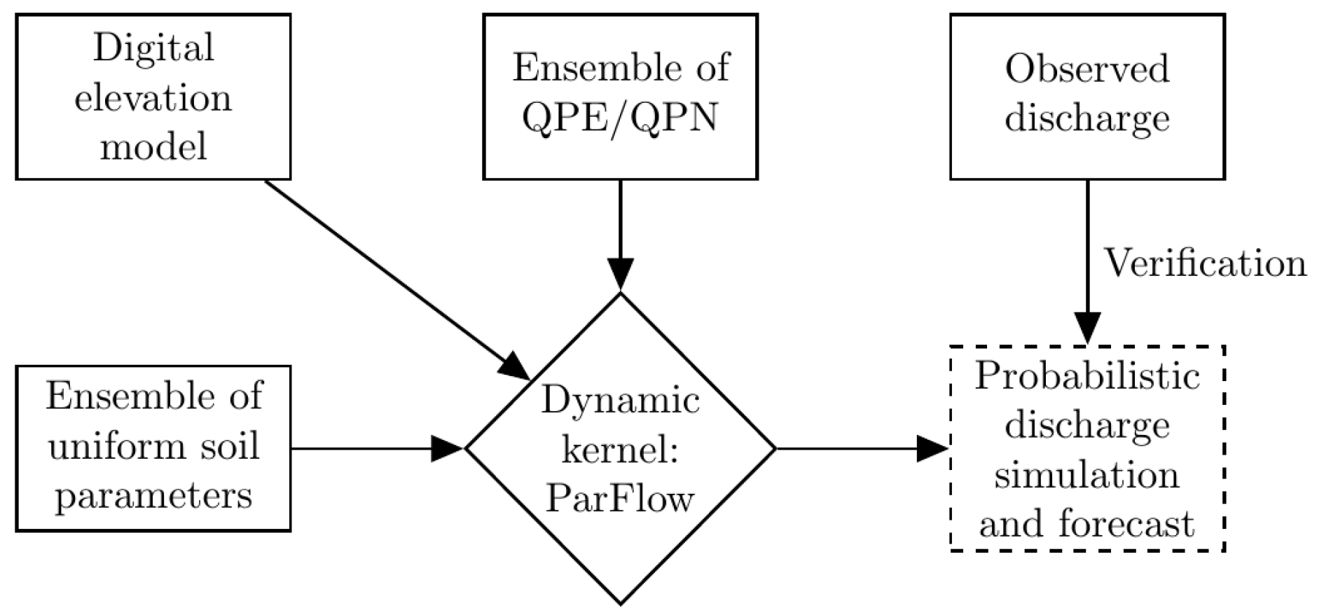
2.1. Framework

The framework encompasses a probabilistic hindcasting and nowcasting system, within which sources of uncertainty are propagated and represented in the result. The main components of the framework, as shown in Figure 1, are the model of the small watershed based on a dynamic kernel, i.e., ParFlow, and the quantitative precipitation estimates (QPEs) and nowcasts (QPNs) from radar observations and forward modeling, respectively. Both components are implemented in an ensemble hindcasting and forecasting system to account for hydraulic parameter and rain input uncertainties. To account for initial soil moisture states at the beginning of the respective event, spinup simulations are performed for each ensemble member and event. The results of the framework are probabilistic forecasts of discharge at any given point along the river corridor.

Based on the rationale that in small catchments, flash flood generation and propagation is mainly determined by processes and less by the spatial heterogeneity of physical parameters, the parsimonious model is informed with spatially homogeneous hydraulic properties. Thus, a total of only seven input parameters (saturated hydraulic conductivity, porosity, specific storage, residual water content, van Genuchten n and α, Manning’s roughness) is required. In this study, the ParFlow model was applied, yet any other PDE-based hydrologic model may be utilized resulting in a similar number of hydraulic parameters depending on the coupling of groundwater with surface water flow. A model ensemble was generated by perturbing the two most sensitive hydraulic parameters at regular intervals along physically reasonable ranges for the area, and subsequently forced with five-minute radar QPE and QPN data. The skill and uncertainty of the framework were assessed by comparing simulated to observed discharge at gauging sites. In order to account for the uncertainty associated with the precipitation input, which constitutes the only time series input into the model, two different QPE products were applied in the ParFlow simulations.

To further test the validity of the proposed framework, ParFlow QPE simulations were compared against simulations using the lumped, conceptual Hydrologiska Byråns Vattenavdelning (HBV) [19,44,45] model for comparison. The model was chosen due to the fact that HBV-type models have been extensively used in modeling sparsely gauged catchments due to their low input data requirements and computational efficiency [46,47,48]. However, 14 catchment-specific model parameters need to be calibrated [19]. In this case, the default automatic calibration was applied. HBV has been applied for flood monitoring and forecasting purposes, as well as flash flood modeling, and studies reported good calibration but sometimes deteriorated validation results [28,29,30,49,50,51].

2.2. Framework Components

2.2.1. The ParFlow Model

The proposed framework builds upon the three-dimensional, variably saturated groundwater flow model ParFlow [38,39,52,53]. It was originally developed at the Lawrence Livermore National Laboratory and first described by [38,52]. Development is ongoing, with a two-dimensional overland flow simulator by [39] and a terrain-following grid transform added by [53]. ParFlow was designed for high-performance computing environments and was shown to scale well in massively parallel applications [38,39,52,53,54,55]. In this section, the underlying model formulations of ParFlow and the free surface overland flow boundary condition, as well as the terrain-following grid transform, will be briefly presented based on [39,53]. Please refer to [38,39,52,53] for further information. Without the application of the terrain-following formulation, ParFlow solves the underlying equations for regular, orthogonal coordinates. Variably saturated three-dimensional groundwater flow is calculated based on the Richards [56] equation:

$$\begin{array}{c}\hfill S_s{S}_w\frac{\partial \psi }{\partial t}+\varphi \frac{\partial S_w\left(\psi \right)}{\partial t}=\nabla ·q+q_r(x,z)\\ \hfill q=\varphi S_w\left(\psi \right)v=-K_s\left(x\right)k_r\left(\psi \right)\nabla (\psi +z)\end{array}$$

(1)

where $S_s$ is the specific storage $\left[L^{-1}\right]$, $S_w$ is the relative saturation $[-]$, $\psi$ is the pressure head $\left[L\right]$, t is the time $\left[t\right]$, $\varphi$ is the porosity $[-]$, q is the specific volumetric Darcy flux $\left[L{T}^{-1}\right]$, $q_r$ is a general source/sink term $\left[L{T}^{-1}\right]$, z is the elevation with the axis specified as upward $\left[L\right]$, v is the subsurface flow velocity $\left[L{T}^{-1}\right]$, $K_s\left(x\right)$ is the saturated hydraulic conductivity $\left[L{T}^{-1}\right]$ and $k_r$ is the relative permeability $[-]$. Relative saturation and permeability are described using [57] functions:

$$S_w\left(\psi \right)=\frac{S_{sat}-S_{res}}{{(1+{\left(\alpha \psi \right)}^n)}^{(1-1/n)}}+S_{res}$$

(2)

$$k_r\left(\psi \right)=\frac{{\left(1-\frac{{\left(\alpha \psi \right)}^{n-1}}{{(1+{\left(\alpha \psi \right)}^n)}^{1-1/n}}\right)}^2}{{(1+{\left(\alpha \psi \right)}^n)}^{\frac{(1-1/n)}{2}}}$$

(3)

where $S_{sat}$ and $S_{res}$ are the relative saturated water content $[-]$ and the relative residual saturation $[-]$, and $\alpha$ $\left[L^{-1}\right]$ and n $[-]$ are soil parameters. In ParFlow, overland flow is introduced via the two-dimensional kinematic wave equation (Equation (4)). Using conditions of continuity of pressure and flux, the equation is included as the boundary condition to the Richards equation at the top of the model:

$$k(-K_s\left(x\right)k_r\left(\psi \right)\nabla (\psi +z))=\frac{\partial \parallel \psi ,0\parallel }{\partial t}-\nabla ·\parallel \psi ,0\parallel v^{sw}+q_r\left(x\right)$$

(4)

where k represents the unit vector in the vertical and h the surface ponding depth $\left[L\right]$, now equivalent to $\psi$ in Equation (1). If $\psi >0$, $q_r\left(x\right)$ $\left[L{T}^{-1}\right]$ becomes the general source/sink term equivalent to $q_r$ in Equation (1). $\parallel \psi ,0\parallel$ indicates the greater of $\psi$ and 0 and $v^{sw}$ is the two-dimensional, depth-averaged surface water velocity $\left[L{T}^{-1}\right]$. The left-hand side of Equation (4) represents vertical fluxes, such as infiltration or exfiltration across the land surface boundary. It is assumed in the overland flow boundary condition that the pressure ($\psi$) represents both surface pressure and ponding depth. Overland flow is generated whenever the pressure head at the land surface is greater than zero, which can be due to either excess infiltration or excess saturation. The flow depth–discharge relationship is then derived using Manning’s equation ($v^{sw}$ in Equation (4)):

$$v_i^{sw}=\frac{\sqrt{S_{f,i}}}{n}{\psi }^{2/3}$$

(5)

where $S_f$ is the friction slope $[-]$, i refers to both x and y directions and n is the Manning’s coefficient $\left[T{L}^{-1/3}\right]$. The friction slope equals the topographic slope $S_0$. By neglecting pressure changes in the x and y directions, Equation (5) can be expressed as the kinematic wave approximation $v_x^{sw}=\frac{\sqrt{S_{0,x}}}{n}{\psi }^{2/3}$. In the above-outlined model formulation, ParFlow uses an orthogonal grid. Topographic information must then be mapped onto this grid. In this case, cells above the land surface are inactive and not included in the solution. The terrain-following transform is applied by extending the orthogonal formulation by including gravity contributions into the Darcy flux (lower part of Equation (1)). This is accomplished by modifying the Darcy flux to locally follow changes in slope. It is assumed that the slope change is uniform over the vertical dimension, i.e., all cells have identical slopes in the z dimension. The lower part of Equation (1) is thus modified to:

$$q=-K_s\left(x\right)k_r\left(\psi \right)[\nabla (\psi +z)cos{\theta }_x+sin{\theta }_x]$$

(6)

where $\theta$$[-]$ represents the local slope angle in the x and y directions and can be expressed as ${\theta }_x={tan}^{-1}\left(S_{0,x}\right)$ and ${\theta }_y={tan}^{-1}\left(S_{0,y}\right)$. The flux, exemplarily given for the x direction here, may now be expressed as:

$$q_x=-K_{s,x}\left(x\right)k_r\left(\psi \right)\frac{\partial \left(\psi \right)}{\partial x}cos{\theta }_x---K_{s,x}\left(x\right)k_r\left(\psi \right)sin{\theta }_x$$

(7)

For a flat surface of $S_{0,x}=0$ and ${\theta }_x=0$, Equation (7) would then reduce to the lower part of Equation (2). The discharge rate Q in $\left[L^3{T}^{-1}\right]$ is calculated externally by multiplying the depth averaged velocity with the flow through area, defined by the ponding depth $\psi$ and the length of the grid cell ${\Delta }_i$:

$$Q_i=v_i^{sw}\psi {\Delta }_i=\frac{\sqrt{S_{f,i}}}{n}{\psi }^{5/3}{\Delta }_i.$$

(8)

2.2.2. Quantitative Precipitation Estimates and Nowcasts

RADOLAN QPE—German Weather Service: The German Weather Service (Deutscher Wetterdienst—DWD) operates a network of 17 c-band radar sites covering the whole of Germany. Radar reflectivity is converted into rain rate and the final precipitation product is released under the name Routineverfahren zur Online-Aneichung der Radarniederschlagsdaten (RADOLAN) mit Hilfe von automatischen Bodenniederschlagsstationen (Ombrometer). The project was launched in 1997 with the goal to provide real time quantitative precipitation estimates. Data are provided in a $1\times 1$ km grid at five-minute and hourly timesteps [58,59].

XPol QPE—University of Bonn: XPol data were supplied by the Hans Ertel Centre for Weather Research—Object-based Analysis and SEamless prediction (HErTZ—OASE) project: www.herz-tb1.uni-bonn.de. The project encompasses the former Meteorological Institute of the University of Bonn (MIUB, now the Department of Meteorology), the Leibniz-Institute for Tropospheric Research (IfT), and the DWD. Two X-band polarimetric doppler radars in combination with DWD RADOLAN data are used to generate the QPE product. One is located in the City of Bonn (BoXPol, 50.731° N; 7.071° E) at an altitude of 99.9 m MSL and one is close to the City of Jülich (JuXPol, 50.927° N; 6.456° E) on an open pit tailings dump at an altitude of 310 m MSL [60]. The surface rain rate used in this study was calculated using the horizontal specific attenuation, which is based on the horizontal reflectivity polarization and the differential propagation phase [60,61,62]. The processed data product was extensively validated [63]. QPE data are given at a spatial resolution of 500 × 500 m and a temporal resolution of 5 min.

RADOLAN QPN—German Weather Service/University Bonn: In our methodology, a nowcast of a given RADOLAN QPE field is obtained using the spectral prognosis approach [64]. This approach is based on the scaling behavior of rain and its scale-dependent predictability property. The latter implies that large spatial scales of rain exhibit a longer lifespan than small ones. First, the method decomposes the rainfall field into a multiplicative cascade of decreasing spatial scales. Second, an autoregressive second-order model is used to consider the evolution of precipitation at each cascade level. Hence, small rain components that are expected to have a short lifespan are filtered. Third, each cascade level is advected using the optical-flow method described by [65]. Lastly, the advected cascade levels are integrated and thereby a deterministic nowcast is obtained. To take into account uncertainties in the nowcast related to the decay and growth of precipitation, the short-term ensemble prediction system (STEPS) method is used [66]. STEPS adds perturbations to each cascade level and the advection field by using Gaussian white noise, which is correlated to the last-observed QPE field. An ensemble of 20 nowcast members is generated for each precipitation event at a spatial resolution of 1 × 1 km and a temporal resolution of 5 min.

2.2.3. Ensemble Generation for Uncertainty Estimation

In order to account for input data and model parameter uncertainty, model ensembles are generated by which the respective uncertainties can be propagated through the forecasting framework. Ensembles of parameter uncertainty are generated by perturbing two, in our case spatially uniform, soil parameters, namely the saturated hydraulic conductivity and the Manning’s roughness coefficient, within physically reasonable ranges. The precipitation input uncertainty is represented by using two different QPE products. For the nowcasts, two-hour long QPN ensembles are spawned every 5 min based on the STEPS methodology and RADOLAN initial rainfields. The QPN ensemble thus encompasses rainfields of perturbed spatial distribution and magnitude. The reader is referred to Section 2.3.2 and Section 2.3.3 for a detailed description of the ensemble generation for the case study.

2.3. Framework Application

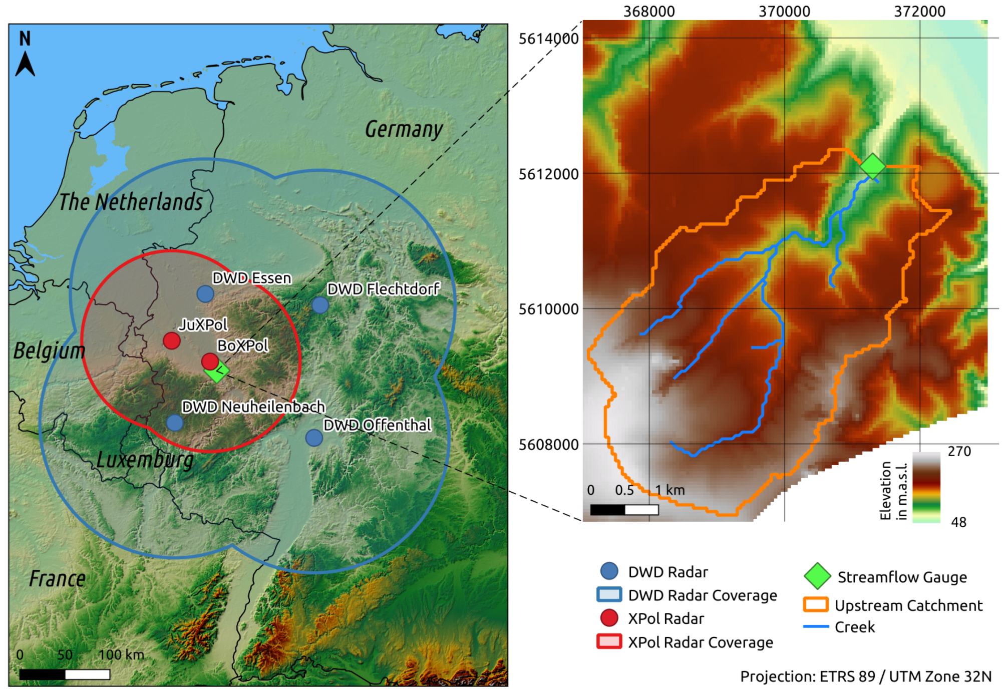
2.3.1. Study Area

The performance of the modeling framework is evaluated over the catchment of the Mehlemer Bach in the south of the City of Bonn in North Rhine-Westphalia, Germany. The catchment contains only a single stream gauge; rain gauges or other in-situ sensors are not available. The catchment is covered by four precipitation radars of the German Weather Service and two radars of the Geoverbund ABCJ (Universities of Aachen, Bonn and Cologne and Research Center Jülich), as seen in Figure 2. The catchment area is 18.5 km² in size, approximately 16.3 km² of which are located upstream of the stream gauge.

The catchment, which drains into the Rhine river, is prone to flash flooding, which has been documented for several hundred years, and has been associated with property damages and sometimes injuries or deaths [68,69,70]. The City of Bonn has implemented early warning and flood alleviation measures, including continuous radar and camera observations of the river stage at the gauge in Niederbachem and the construction of a canal to divert flood water into the Rhine [71]. Recent flood events, which are covered by the available data products, took place on 3 July 2010, 20 June 2013 and 4 June 2016 [69,70], and were included in the analysis (see also

Table 1. Events examined for the Mehlemer Bach catchment.

		Discharge Levels Exceeded
Event	Qmax in m3 s−1	Level 1	Level 2
3 July 2010	49.98	y	y
20 June 2013	27.07	y	y
30 May 2016	2.77	n	n
1 June 2016	3.65	n	n
4 June 2016	24.80	y	y

Notes: Q_max: maximum discharge reached during the event; Level 1 is reached at 4.5 m³ s⁻¹; Level 2 is reached at 15 m³ s⁻¹. y: yes; n: no.

). Additionally, two cases that did not lead to flooding were included in the experiment to assess how well the model can propagate non flood-inducing rainfalls. For this catchment, two flood discharge levels were defined: Level 1, at a discharge rate of 4.5 m³ s⁻¹, corresponds to a water level of one meter and is reached when the channel is half full at the gauge. It is assumed that if this level is surpassed, the potential for the formation of a flood wave exists. Level 2 is reached at a discharge rate of 15 m³ s⁻¹ and corresponds to a nearly bankfull channel. It is assumed that such discharge rates may lead to severe flooding. River discharge data at the Niederbachem stream gauge (50.646° N, 7.179° E) is provided by the Community of Niederbachem in cooperation with the City of Bonn and the Ministry for Environment, Agriculture, Conservation and Consumer Protection (LANUV) of the State of North Rhine-Westphalia. The water level gauge only records changes in the water height. Discharge is calculated based on an empirical stage–discharge relationship. The long-term (1992–2016) average discharge at the gauge is 0.09 m³ s⁻¹ with a standard deviation of 0.12 m³ s⁻¹. Level 1 was exceeded on nine days during this period, while Level 2 was exceeded only on the three days mentioned above.

2.3.2. ParFlow Model Setup

The computational grid is set up based on a sink-filled 50 m spatial resolution digital elevation model resulting in 122 cells in the x direction, and 156 cells in the y direction, covering an area of approximately 48 km². In the vertical dimension, four layers are defined with thicknesses of 20 cm, 1 m, 2 m and 4 m, leading to an overall depth of the model domain of 7.20 m. This is considered to approximate the upper horizons of the watershed sufficiently for performing terrain-following grid simulations and honoring fast subsurface runoff. Since the gauging station is located almost in the middle of a single model grid cell, only this cell needs to be considered to extract the modeled discharge. No-flow boundary conditions are applied at the bottom and perimeter of the domain, while an overland flow boundary condition is implemented at the top. The lateral boundary conditions are placed far beyond the watershed boundaries in order to simulate dynamic water divides. The model is informed with the following spatially homogeneous hydraulic parameters: the saturated hydraulic conductivity, the van Genuchten parameters, porosity and storativity, and Manning’s roughness; resulting in a total of only seven parameters. As mentioned above, while ParFlow was applied in this study, the application of any other PDE-based hydrologic model will result in a similar number of hydraulic parameters in a parsimonious setup. Spinup simulations were performed for each ensemble member assuming individual long-term averaged recharge rates to account for the initial soil moisture states at the beginning of the respective event, which strongly influence the runoff response [34]. Each spinup was run at 10-h timesteps over a period of 10 years. A simulation timestep of 5 min was applied based on the available QPEs. As the radar data is supplied in a polar stereographic projection, mapping to the regular ParFlow grid was performed using the wradlib Python library by [72].

In order to obtain a measure of the parameter uncertainty, an ensemble was generated by perturbing the surface roughness n and saturated hydraulic conductivity $K_s$ parameters, as shown in

Table 2. Parflow ensemble members and their parameters.

		${\mathit{K}}_{\mathit{s}}$
		0.015	0.02	0.03	0.05
	$1.5\times {10}^{-5}$	0_1	0_2	0_3	0_4
n	$1.0\times {10}^{-5}$	1_1	1_2	1_3	1_4
	$5.0\times {10}^{-6}$	2_1	2_2	2_3	2_4

Notes: n: Manning’s n $\left[T{L}^{-1/3}\right]$; $K_s$: Saturated hydraulic conductivity $\left[L{T}^{-1}\right]$.

. Values were confined to physically reasonable ranges for the study area and sampled at regular intervals. According to the United States Department of Agriculture (USDA), $K_s$ values of 0.015, 0.02 and 0.03 m·h⁻¹ constitute loam, silt loam, silt, and sandy clay loam soils, where the runoff potential is moderately low. At 0.05 m·h⁻¹, the runoff potential is low. Possible soil textures include loamy sand, sandy loam, loam and silt loam [73]. Manning’s n values $\left[T{L}^{-1/3}\right]$ were set at 1.5 × 10⁻⁵, 1.0 × 10⁻⁵ and 5.0 × 10⁻⁶, which correspond to stony, vegetated creeks, natural riverbeds with rubble and earth channels in solid soils, respectively. The decrease in the values corresponds to an increase in flow velocity as the surface roughness reduces [74,75,76].

2.3.3. Hindcasting and Nowcasting Experiments

Three types of numerical experiments were performed, namely a hindcast experiment, a zero precipitation forecast experiment and a nowcast experiment. In the hindcast experiment, the spun-up model was forced for each of the five precipitation events and 12 ensemble members. This was done in order to verify whether the model is capable of reproducing the observed streamflow within the catchment. We added two precipitation events that did not lead to flooding to verify the capability of the model in simulating non-flood streamflows. The model ensemble was applied to account for the parameter uncertainty. Input data uncertainty was addressed by forcing the model with two different 5-min QPEs: RADOLAN and XPol.

In the zero precipitation forecast experiment, three-hour forecasts of the flood events are spawned every 5 min using the last prediction step of the initial model as the initial condition. Here, it was assumed that no more precipitation takes place in order to evaluate which lead times can be achieved using this model setup. This was performed for both RADOLAN and XPol QPEs.

In the nowcast experiment, RADOLAN-based QPNs were used to force the model during a two-hour long nowcast spawned every 5 min. This was done to test the quality of the forecasted precipitation information and to evaluate whether lead times can be further increased. To properly evaluate the nowcast performance, a nowcast must be run for each model ensemble and each nowcast ensemble member. Since this would lead to a very large number of simulations, it was decided to choose five out of the 20 available nowcast members (1,5,9,13,17) for this analysis. As the ensemble simulations are of a probabilistic nature, the continuous ranked probability score ($CRPS$) was used in addition to commonly-used deterministic indices to evaluate the model skill. $CRPS$ is the integral of the Brier score for an infinite number of thresholds, and it accounts for the reliability and sharpness of the predictive ensemble distribution. A sharp forecast is attained if high forecast reliability coincides with the observation, whereas the forecast probability is minimal for other events. It is used to assess the quality of ensemble and probabilistic forecasts. For point forecasts, it reduces to the mean absolute error ($MAE$), allowing for a direct comparison between both forecast approaches [77,78]. According to [78], $CRPS$ is calculated as:

$$CRPS(F_t,x_t)={\int }_{-\infty }^{\infty }{(F_t\left(x\right)-H(x\ge x_t))}^{2}dx$$

(9)

where $F_t$ represents the predictive cumulative distribution function for day t, x is the predicted variable and $x_t$ the observed variable. $H(x\ge x_t)$ is the Heavyside function that equals 1 if the predicted values are above the observation and 0 if below. The $CRPS$ score is not bounded on the upper side and a perfect score is indicated by zero. In order to calculate the standard deviation of the $CRPS$, a jackknife technique was applied, where the mean score is calculated for the number of ensemble members by excluding one member each time. Then, the standard deviation of the resulting values was calculated, as proposed by [78].

2.3.4. Comparison with the Lumped Conceptual HBV Model

To assess the added value of using the PDE-based ParFlow model for probabilistic flash flood forecasting purposes, the model setup and key results were compared against results achieved by applying the conceptual, lumped HBV [19,44,45] model, which simulates discharge based on time series of precipitation, temperature and evapotranspiration. For an in-depth description of the model, please refer to [45,79].

A lumped HBV model was constructed where precipitation is averaged over the entire catchment, and the model was calibrated against observed discharge at the Niederbachem gauge. While it is possible to run HBV in a distributed way by defining multiple subcatchments, this is not meaningful, because only one discharge gauge is available for calibration. Additionally, it is common practice to calibrate headwater catchments separately to avoid inflow and routing uncertainties [46]. For flood analysis and forecasting, the model is typically run at hourly timesteps [29,30,49,80]. The authors realize that calibrating an area-averaged model using only one stream gauge will have an effect on the results. Strong local rainfall rates will be spatially smoothed, leading to reduced precipitation peaks and different wave celerities. However, due to the hourly resolution of the model and small spatial scale of the catchment, these issues are minor. For a robust calibration, extended time periods of observed discharge covering various hydrologic conditions are important. It becomes obvious, therefore, that the HBV model cannot be robustly calibrated using the observations of only five precipitation events. Hence, a long-term calibration using hourly gauge-corrected RADOLAN QPEs was performed. According to QPE and discharge data availability, the periods for model spin-up and calibration were defined as 2006–2009 and 2010–2016, respectively. Hourly RADOLAN QPEs were extracted and averaged over the catchment using wradlib. In addition to precipitation information, HBV requires observations of the average air temperature (to calculate snowfall) and evaporation [44]. Temperature data were extracted from the DWD station Bonn-Rohleber located approximately 10 km to the northeast of the study area, and daily potential evapotranspiration data were provided at a 1 km resolution by the DWD and averaged over the study area [81]. The model was automatically calibrated for the 14 default parameters based on the the $NSE$ efficiency criterion using the default genetic algorithm and Powell [79] (GAP) approach. By default, the model is optimized using 5000 genetic algorithm runs to find the best parameter combination, which is followed by 1000 Powell optimizations to find the local minimum [82]. Since all model parameters were included in the calibration and the final parameter value was not of interest to this study, no sensitivity analysis was performed. Due to the low occurrence of high flows in the catchment, two calibration options were explored. In the first, the model was calibrated without all five validation events, and in the second, it was calibrated for each event individually by excluding the day in question but including all other events. The calibrated models were then validated for the days not included in the calibration.

3. Results and Discussion

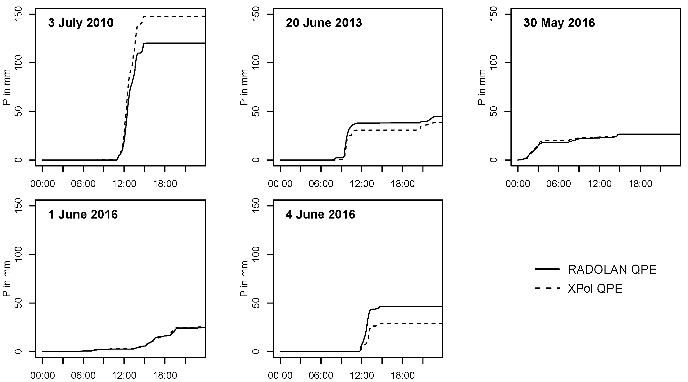
3.1. Radar QPE Uncertainty

There is general agreement that the precipitation input uncertainty is higher than the model parameter uncertainty [28,29,51]. Two different radar QPEs were chosen to represent the input data uncertainty in this study: RADOLAN and XPol. Rain rates derived from the QPEs averaged over the catchment for the five precipitation events are presented in Figure 3 and

Table 3. Comparison of XPol and RADOLAN radar QPEs.

			$\mathit{RMSE}$	Total
Event	${\mathit{R}}^2$	$\mathit{PBIAS}$	(mm/5 min)	RAD	XPol
3 July 2010	0.92	22.9	0.50	120	148
20 June 2013	0.59	−14.1	0.43	45	39
30 May 2016	0.83	−2.0	0.09	27	26
1 June 2016	0.70	3.7	0.11	25	26
4 June 2016	0.50	−37.4	0.44	47	29

Notes: R²: Coefficient of determination; PBIAS: Percent BIAS; RMSE: Root mean squared error; RAD: RADOLAN; Total: Total precipitation in mm.

. Generally, both products compared well over the Mehlemer Bach catchment with a mean $R^2$ score of 0.71 and $RMSE$ of 0.31 mm per 5-min measurement interval. For the two non-flood events (30 May 2016 and 1 June 2016), estimated rain rates were almost identical between both products. With an increase in the rain rate, differences became apparent. For both 20 June 2013 and 4 June 2016, XPol estimated less precipitation, while for the event with the highest rain rate, 3 July 2010, RADOLAN estimated less precipitation. This may be explained by the characteristics of the respective radar systems and the retrieval algorithms applied in the different products. Overall, the radar estimates compared better during lower precipitation events and biases increased with an increase in precipitation.

3.2. Model Results

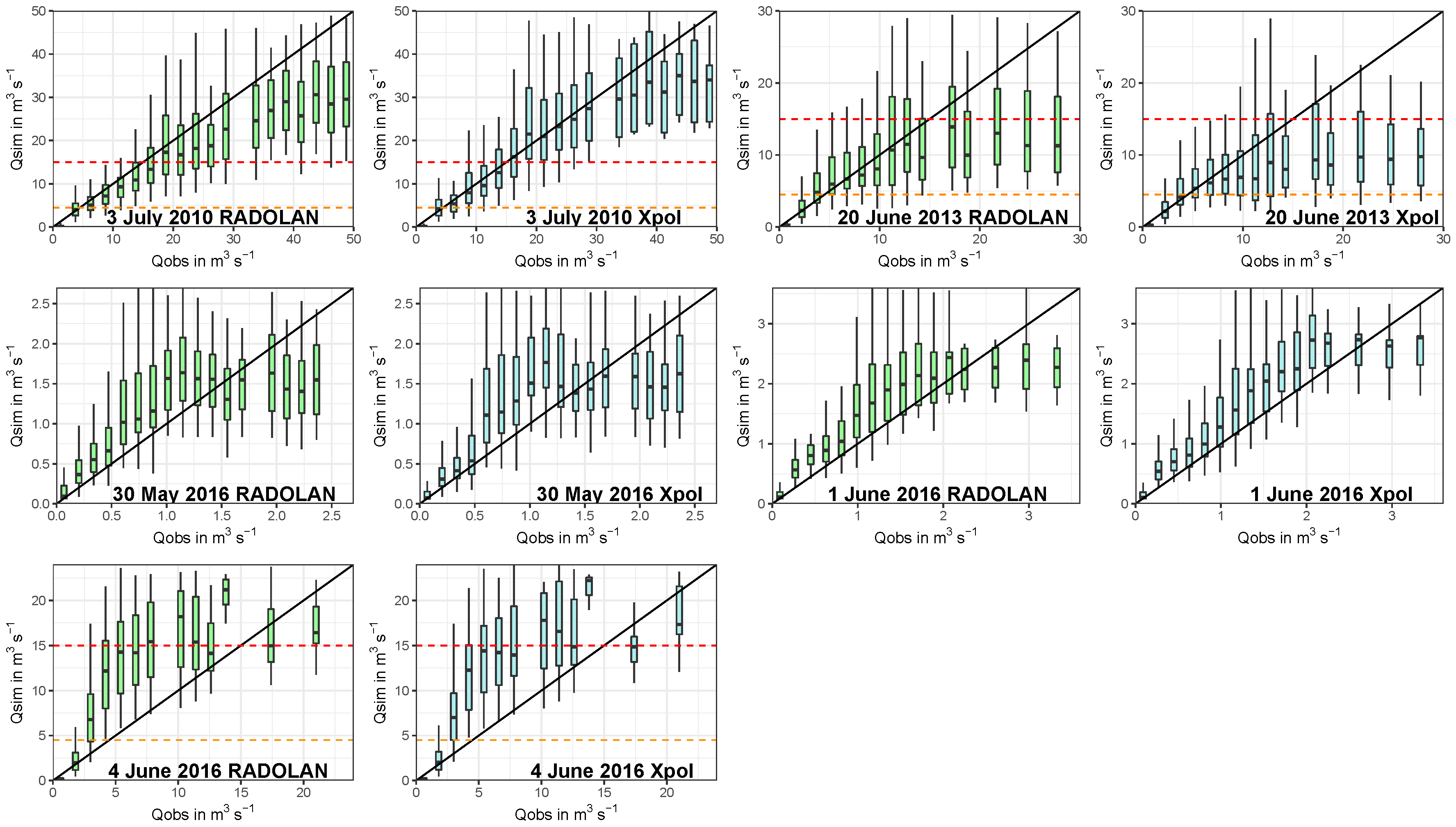
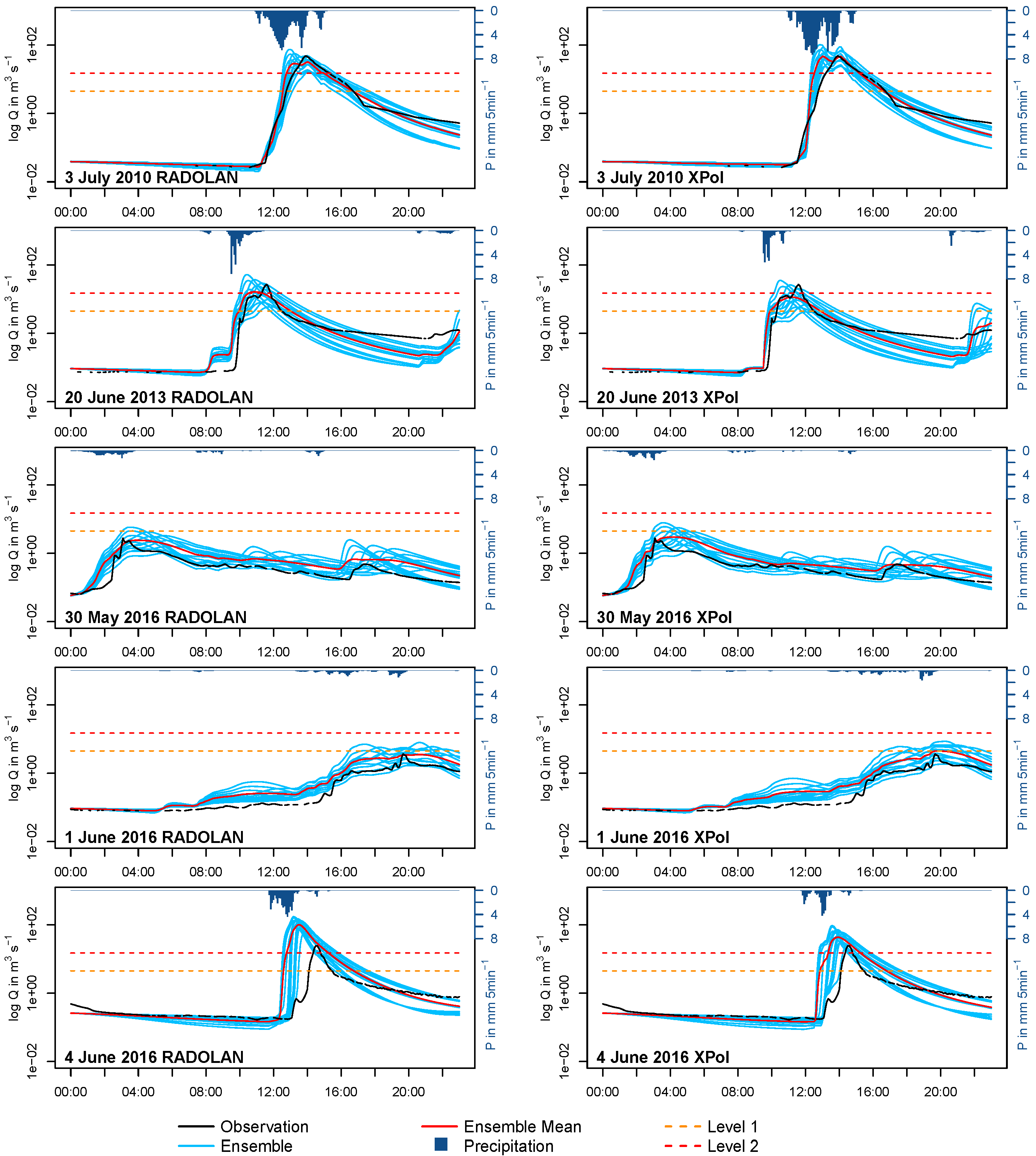
3.2.1. ParFlow Hindcast Experiment

In the following, the results of the ParFlow hindcast experiment forced with both RADOLAN and XPol QPEs are presented for all five events. While the simulated discharges are presented in Figure 4, accompanying statistics describing the performance of the ensemble and ensemble mean are given in

Table 4. ParFlow reanalysis ensemble performance.

		% of obs.			Ensemble Mean Performance
		Bracketed	$\overline{\mathit{CRPS}}$	$\mathit{MAE}$	${\mathit{R}}^2$	$\mathit{NSE}$	$\mathit{PBIAS}$	$\mathit{RMSE}$
RADOLAN	3 July 2010	56	0.760 (0.047)	1.267	0.85	0.85	−5.9	3.46
	20 June 2013	37	0.588 (0.016)	0.826	0.78	0.78	4.8	1.93
	30 May 2016	57	0.193 (0.014)	0.353	0.81	−0.03	75.7	0.45
	1 June 2016	38	0.243 (0.025)	0.461	0.91	−0.02	84.1	0.73
	4 June 2016	57	4.007 (0.147)	5.817	0.07	−28.64	374.0	19.18
	Mean	49	1.158 (0.050)	1.745	0.68	−5.41	106.5	5.15
XPOL	3 July 2010	48	1.056 (0.063)	1.544	0.75	0.59	31.2	5.71
	20 June 2013	41	0.613 (0.016)	0.698	0.81	0.77	−14.3	1.95
	30 May 2016	76	0.193 (0.013)	0.342	0.80	−0.63	74.1	0.56
	1 June 2016	33	0.274 (0.028)	0.511	0.94	−0.37	93.7	0.85
	4 June 2016	57	1.697 (0.084)	2.760	0.36	−4.37	172.9	8.17
	Mean	51	0.767 (0.041)	1.171	0.73	−0.80	71.5	3.45

Notes: % of obs. bracketed: Percentage of observations bracketed in the ensemble uncertainty; CRPS: continuous ranked probability score; MAE: mean absolute error; R²: coefficient of determination; KGE: Kling–Gupta efficiency; NSE: Nash–Sutcliffe efficiency; PBIAS: percent bias; RMSE: root mean squared error. CRPS, MAE and RMSE given in m³ s⁻¹. Standard deviations of CRPS estimated using the jackknife technique are given in brackets.

. Results relating to the ensemble uncertainty are graphically presented in Figure 5.

Overall, with the exception of an apparently strong overestimation of the discharge in the 4 June 2016 case, the model ensembles forced with both XPol and RADOLAN QPEs compared well to the observed discharge. As was done by Boucher et al. [78], $MAE$ was calculated using the 5-min ensemble mean as a point simulation, while the $\overline{CRPS}$ was calculated by taking the ensemble mean of the $CRPS$ at each timestep. This way, the $MAE$ can be compared to the $CRPS$. A perfect score for both would be indicated by zero. For all five events and two QPE forcings, the $\overline{CRPS}$ was lower than the $MAE$, indicating that the ensemble has an overall higher skill than the ensemble mean, highlighting the advantage of applying a probabilistic approach over a deterministic one [78].

The choice of QPE forcing impacts the overall model performance. For all events except 4 June 2016, the $\overline{CRPS}$ of the RADOLAN forced model performed better by an average of 0.088 ${\mathrm{m}}^3{\mathrm{s}}^{-1}$, which is higher than the standard deviation of the $\overline{CRPS}$ calculated using the jackknife approach for the first five events. This indicates a higher contribution of the forcing uncertainty to the overall model uncertainty. For the 4 June 2016 flood event, both models estimated the onset of peak flow early, with the RADOLAN forced model performing worst. Here, RADOLAN $\overline{CRPS}$ was more than double that of the XPol result. Ensemble members (Table 2) with higher $K_s$ parameters, such as 0_4, 1_4 and 2_4, simulated less discharge, as water percolates more quickly. On the other hand, members with lower hydraulic conductivities, such as 0_1, 1_1 and 2_1, generated more discharge, which is intuitive. Manning’s coefficient parametrizes the surface roughness of the catchment, influencing the flow velocity. In members with lower n values (e.g., 2_1, 2_2, 2_3 and 2_4), the flood wave will reach the gauge earlier, due to an increase in flow velocity caused by the reduced roughness, while in members with increased roughness (e.g., 0_1, 0_2, 0_3 and 0_4), the flood wave will reach the gauge later. Because of the heterogeneity of precipitation events that lead to flooding, no single ensemble member parametrized all analyzed flood events well, with best-performing members varying on a case-by-case basis. This highlights the value of using an ensemble simulation approach versus a deterministic approach. Two events that did not lead to flooding were included in the ParFlow analysis experiment to test how well the model performs in these cases. Results show that while a few ensemble members surpassed the first discharge level, the ensemble mean reproduced the catchment behavior adequately, albeit with some overestimation, as can be seen in Table 4 and Figure 4.

On average, 50% of observations were bracketed by the model parameter uncertainty for both RADOLAN and XPol forcings. For ease of interpretation of the ensemble and forcing uncertainty, results are categorized into equidistant bins and plotted as conditional quantiles in Figure 5, according to [83], with the angle bisector indicating a theoretical perfect fit between model result and observation. Especially when focusing on the streamflows below the second warning level, where the discharge curve becomes unreliable due to overbank flow, we observed a good fit of the models to the observations, with the perfect fit being encompassed by the interquartile range for the 3 July 2010 and 20 June 2013 events and included in the 1.5 times interquartile range for the 30 May 2016 and 1 June 2016 events. As expected, the fit was worst for the 4 June 2016 event, showing high overestimations.

Furthermore, basin response times were evaluated for the flood cases (

Table 5. ParFlow hindcast basin response times for flood events.

		Ensemble
	Obs.	Min.	Mean	Max.
3 July 2010
XPol	1:30	0:25	0:35	1:40
RADOLAN	1:25	0:30	1:30	1:35
20 June 2013
XPol	2:00	0:55	1:35	2:30
RADOLAN	2:05	0:50	1:20	2:20
4 June 2016
XPol	1:35	0:35	0:55	1:35
RADOLAN	1:45	0:20	0:40	1:05

Notes: Obs.: Observed hydrograph; Min.: minimum response time of ensemble simulation; Mean: response time of ensemble mean; Max.: maximum response time of ensemble simulation. Response time is defined as the time between precipitation and discharge peak.

). Basin response times are defined here as the time between rainfall and discharge peaks of the observations and different models. During the 3 July 2010 event, the observed basin response time was 1:25 (h:min) for the RADOLAN and 1:30 for the XPol QPE. Simulated response times bracketed the observations. The RADOLAN-forced ensemble mean matched the observations closely, with a time difference of only 5 min, while the XPol ensemble mean simulated a much shorter response time of only 0:35 after the precipitation peak. During the 20 June 2013 event, observed response times resembled each other again closely, at 2:05 (RADOLAN) and 2:00 (XPol). Again, simulations bracketed these well. The ensemble means, however, reflected a faster arrival of the flood wave, with mean response times of 1:20 (RADOLAN) and 1:35 (XPol). Both QPEs had response times of 1:45 and 1:35 during the 4 June 2016 event, respectively. In this case, model simulations did not bracket these times well, with the latest discharge peak of the RADOLAN forced models simulated at 1:05 and and 1:35 for the XPol forced models. Consequently, ensemble mean response times were too fast at 0:40 and 0:55, respectively, indicating unrealistic model behavior. In general, the response time uncertainty introduced into the simulations through the different forcing products was low if the whole ensemble range was observed. However, ensemble mean response times varied considerably.

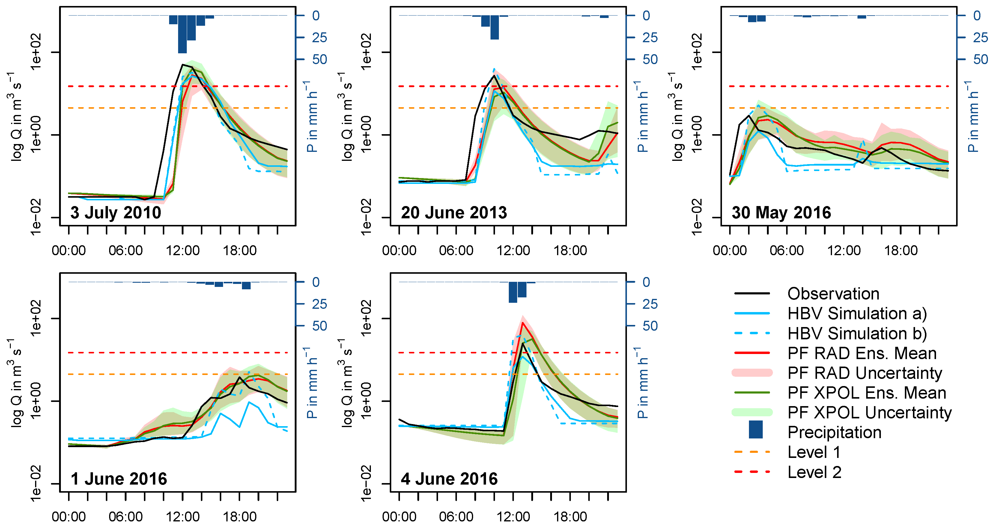
3.2.2. Comparison with HBV Hindcasts

In the following, the results of the HBV hindcast experiment forced with both RADOLAN and XPol QPEs for all five events are presented for comparison. For the first calibration, (a), the HBV model was calibrated from 2010 to 2016 without the five validation events, while for the second calibration, (b), the model was calibrated for each flood event individually. HBV calibration (a) did no reach acceptable $R^2$ or $NSE$ values with 0.32 and 0.31, respectively. The averaged performance of the five models of calibration (b) performed better, with an $R^2$ of 0.74 and $NSE$ of 0.71.

Validation results are shown in Figure 6 and

Table 6. HBV and ParFlow ensemble statistics.

	HBV MAE in m3 s−1		ParFlow $\overline{\mathit{CRPS}}$ in m3 s−1
	Simulation (a)	Simulation (b)	RADOLAN	XPOL
3 July 2010	3.206	2.300	3.501	3.063
20 June 2013	1.706	1.499	1.821	1.857
30 May 2016	0.312	0.483	0.489	0.500
1 June 2016	0.517	0.436	0.436	0.489
4 June 2016	0.948	2.384	4.268	1.798
Mean	1.338	1.420	2.103	1.541

Notes: MAE: Mean Absolute Error; $\overline{CRPS}$: Mean Continuous Ranked Probability Score. CRPS reduces to MAE for deterministic simulations, allowing for a direct comparison.

, with ParFLow hindcast results aggregated to hourly values included for comparison. Peak flows were consistently underestimated during simulation (a), with a mean $PBIAS$ of −48.5. Due to the fact that very few high precipitation events occurred during the calibration period, the model could not be robustly calibrated when the five high precipitation events were excluded from the calibration. Average $NSE$ was also below acceptable at 0.37, while $R^2$ was acceptable at 0.61. When the model was calibrated for each flood event individually under simulation (b), discharge was represented more realistically, albeit with a general overestimation of 11.5 %. $NSE$ performed poorly at −0.14, while $R^2$ was acceptable at 0.66. In comparison, hourly aggregates of ParFlow ensemble mean results overestimated discharge with a mean $PBIAS$ of 38.4 (RADOLAN-forced) and 16.86 (XPol-forced). $NSE$ was below acceptable in both cases (−0.85 and 0.078), while $R^2$ was acceptable at 0.58 and 0.51, albeit lower than the HBV result.

Since the continuous ranked probability score reduces to the mean absolute error for deterministic simulations, the probabilistic ParFlow ensemble performance can be directly compared to HBV results, as done in Table 6. For the case study days 20 June 2013, 30 May 2016 and 1 June 2016, all models performed similarly. For the 3 July 2010 flood case, the HBV simulation (b) outperformed the others. In the 4 June 2016 case, the HBV simulation (a) performed best, followed by XPol-forced ParFlow, HBV Simulation (b) and the RADOLAN-forced ParFlow. When averaged over all case study days, HBV (a), (b) and XPol-forced ParFlow performed similarly, with RADOLAN-forced ParFlow performing less well due to the overestimation of the 4 June 2016 event. The overestimation was less pronounced in HBV simulations, since in tem the hourly, gauge-corrected RADOLAN QPE was applied as opposed to the uncorrected 5-min product used in ParFlow. In conclusion, the ParFlow model performed well in comparison to HBV, given that the model was uncalibrated and originally run at a 5-min timestep with results later aggregated to hourly data, which led to a shift in peak flows due to the employed averaging.

Overall, the experiment highlighted that the HBV calibration of the Mehlemer Bach catchment requires long observational time series over a diverse range of hydrologic conditions in order to better represent single events during the validation. Even if the model is calibrated over long periods of time at hourly timesteps, the calibration remains sensitive to high precipitation events. Flash floods in the area are relatively rare and a good database over a long period of time must exist so as to include as many hydrologic conditions in the calibration as possible. If multiple extreme events are excluded, as was done during calibration (a), the model cannot robustly simulate flood occurrences. Even though most of the validations did not produce acceptable $NSE$ values, all flood event validations of simulation (b) correctly simulated the discharge exceeding both discharge levels and reasonably depicted the discharge dynamics. By contrast, the PDE-based ParFlow model achieved acceptable results without the need for calibration. In contrast to to the conceptual model, it can be applied in catchments where no prior observations are available and delivers results for any point along the river corridor, while HBV needs to be recalibrated for every gauge location. The computational demand of both models should also be taken into consideration. The calibrated HBV model can simulate an event spanning an entire day in under one second on one core. The spun-up ParFlow model, which is run on 48 cores, requires approximately 6 min to do so, while 2-h nowcasts can be simulated in approximately 30 s. In this study, the ParFlow model was applied to a small, 18.5 ${\mathrm{km}}^2$ headwater catchment, for which a total number of 76,128 grid cells (unknowns) needed to be solved in the three-dimensional domain. The model has proven its excellent scalability for problems with up to 8.0 × 10⁹ unknowns in a massively parallel setup [54], and has been applied over a large range of watersheds with complex terrain up to the continental scale, e.g., over Europe with $2.77\times {10}^6$ unknowns [84] and the continental United States with $3.15\times {10}^7$ unknowns [85].

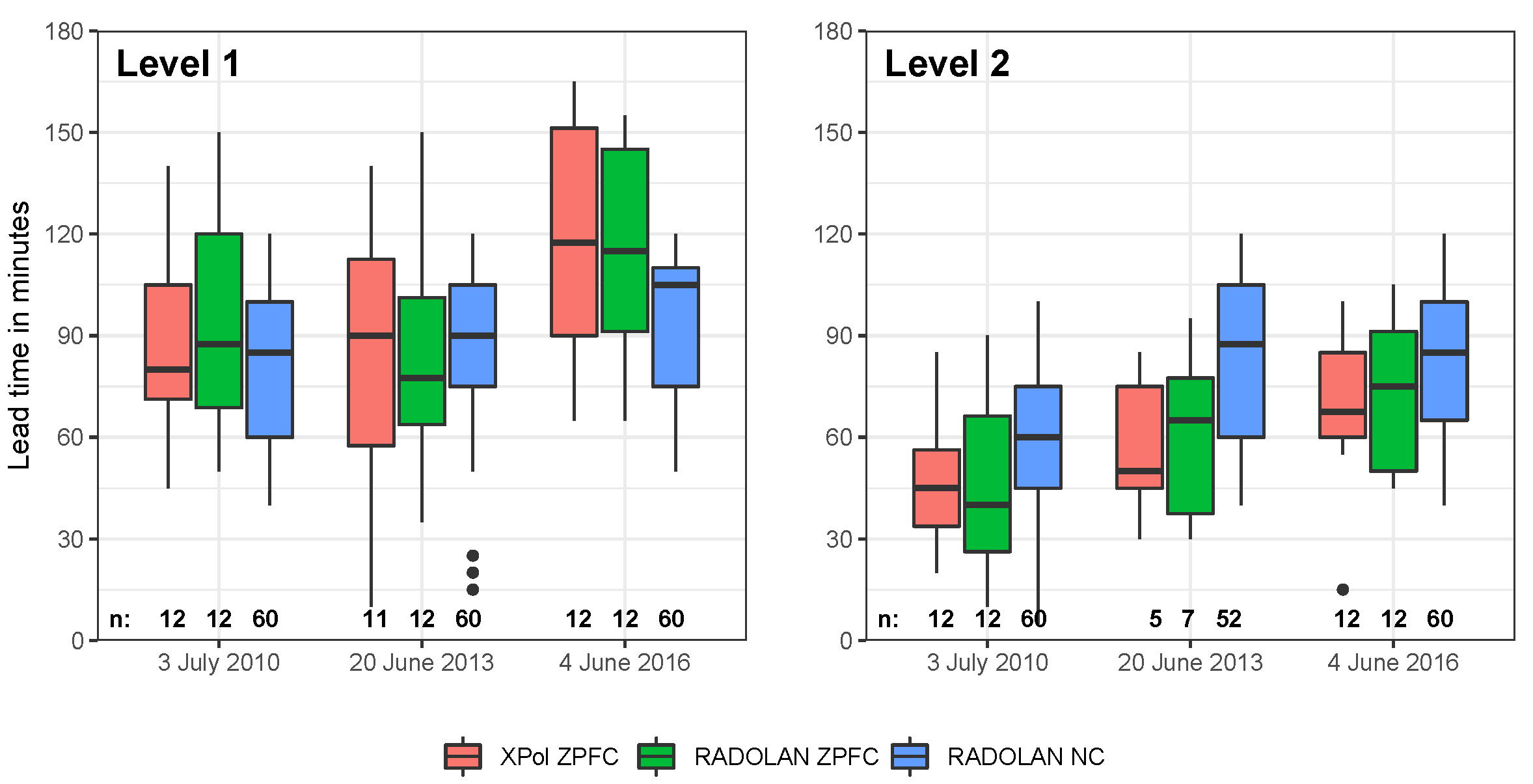
3.2.3. ParFlow Zero Precipitation Forecast and Nowcast Experiment

In the following, the performance of the ParFlow flash flood nowcast experiments will be evaluated in terms of lead time and $CRPS$ compared to observations. Results for both zero precipitation forecasts (ZPFC) forced with XPol and RADOLAN QPE and nowcasts (NC) forced with RADOLAN-based QPN are given in Figure 7 and

Table 7. Ensemble skill analysis for nowcast experiments.

	XPol ZPFC	RADOLAN ZPFC	RADOLAN NC
	$\overline{\mathit{CRPS}}$	$\overline{\mathit{CRPS}}$	min $\overline{\mathit{CRPS}}$	mean $\overline{\mathit{CRPS}}$	max. $\overline{\mathit{CRPS}}$
3 July 2010	2.256	2.355	1.328	1.424	1.485
20 June 2013	1.136	1.052	0.726	0.735	0.745
4 June 2016	0.995	1.708	2.108	2.269	2.440

Notes: ZPNC: zero precipitation forecast; NC: nowcast; CRPS: continuous ranked probability score in m³ s⁻¹.

. While the ZPFC ensembles are built solely on perturbed hydraulic parameters (12 ensemble members), the RADOLAN NC ensemble is built on perturbed hydraulic parameters and five different nowcast realizations (60 ensemble members). The nowcasting period for the ZPFC is three hours, while it is two hours for the NC.

Here, lead time is defined as the time between the start of the nowcast, which eventually exceeds the respective discharge level, and the exceedance of the discharge level by the nowcast. Lead times up to Level 1 (L1) were higher than up to Level 2 (L2), with an average of 94 compared to 64 min for all events and experiments. Concerning the L1 analysis, lead times of the three different ensembles were comparable at 81–95 min for the first two events. The nowcast, however, estimated a shorter lead time for the 4 June 2016 event by around 20 min. This may be explained due to the fact that the NC nowcast period is one hour shorter than the ZPFC period. As can be seen, all NC results ceased at 120 min. For the L2 nowcasts, the NC ensemble consistently outperformed the zero precipitation ensembles, with a mean lead time of 75 min as opposed to around 59 min for both ZPFC ensembles, indicating a realistic prediction by the nowcasting algorithm. For the 2013 flood, not every ensemble correctly indicated surpassing the L2 level.

The model skill is shown in Table 7. $CRPS$ was calculated for each of the nowcasts spawned every 5 min and then averaged to one value. While for the XPol and RADOLAN ZPFC simulations, a single twelve-member ensemble was run, five twelve-member ensembles were run during the RADOLAN NC simulations, based on the five NC realizations used. We therefore give a $CRPS$ range and mean value for these five ensemble simulations. With the exception of the 4 June 2016 event, the nowcast outperformed the zero precipitation forecasts in terms of $CRPS$, with even the worst-performing nowcast realization producing lower errors. For the 4 June 2016 event, the low skill of our model forced with the RADOLAN product becomed apparent, with a higher error of the RADOLAN ZPFC than the XPol ZPFC. In this case, the forecast of rainfall fields given by the nowcasting technique did not reflect reality well, and the performance of the nowcast was lower than the performance of the zero precipitation forecast.

4. Conclusions

In this study, the performance of the proposed flash flood modeling framework was analyzed using the PDE-based ParFlow hydrologic model for a small-scale catchment in Germany. Contrary to the conceptual models generally used for these applications, we highlighted the possibilities of using a parsimonious setup of the model with an ensemble of uniform soil parameters to simulate flash flood events in a small headwater catchment in Germany.

While PDE-based models are often rejected on grounds of complexity and high data requirements, our results show that a PDE-based model can be applied in a flash flood modeling framework, delivering reasonable results considering the low amount of input data, high level of abstraction, such as uniform hydraulic parameters, and lack of calibration. The good performance can be explained due to the fact that the hydrodynamics are realistically simulated at the required temporal and spatial scale. Perturbing key model parameters along physically meaningful values is advantageous, as model parameter uncertainties are thus propagated through the modeling system and represented in the results. However, precipitation input uncertainty constitutes the largest part of the uncertainty, as has been shown before. The key advantage of using a PDE-based model is its ability to be applied without calibration while delivering robust results; additionally, due to its distributed nature, its results are valid for any point along the river corridor. Furthermore, due to the probabilistic design of the experiments, uncertainties can be propagated through the modeling ensemble to be represented in the result. To highlight the added value of using a PDE-based model, the commonly-used conceptual HBV model was also applied to the region. Performance results between the models were comparable, but while the HBV models were extensively calibrated, the ParFlow ensemble was not. This exercise highlights the difficulties associated with conceptual hydrologic models in flash flood studies, as the models need to be calibrated over a long period of time covering various hydrologic conditions. Even a model with a high calibration score thus might not simulate previously unencountered conditions well.

Preliminary nowcast experiments were performed in ParFlow using both precipitation inputs in a zero precipitation forecast, where no further precipitation was assumed during the forecast period. Results showed that even with such a simple assumption, flood wave arrivals can be predicted with average lead times of about 59 min. Including precipitation nowcast ensembles in the framework increases the lead time to up to 75 min and reduces the continuous ranked probability score in most cases.

Overall, this study demonstrates the applicability of the proposed flash flood modeling framework and highlights the advantages of using a PDE-based hydrologic model. Further research is necessary to properly assess the uncertainty associated with QPEs and QPNs in space and time. It is important to note that the uncertainty of the observed discharge was not addressed in this study, but can be considered to be high, particularly whenever overbank flow occurs [86]. Due to the limited data availability and rare occurrence of flash floods in the area, only three flash flooding events and two high precipitation events were examined. In order to expand the usage of the presented framework, the transferability of the framework to other catchments needs to be demonstrated. In the RealPEP project, the framework will be applied to the Bode and Ammer river catchments in Germany, where the effects of spatially distributed soil information and discharge evaluation at multiple gauges will also be examined. Furthermore, the possibility of assimilating observations such as discharge and soil moisture into the model will likely decrease the uncertainty levels of the forecast. In the future, the framework will be used as a platform to evaluate further QPE and QPN products, which are currently being developed within the RealPEP project. Eventually, an online system will be developed where radar QPEs and automatically generated QPNs are directly implemented in a running PDE-based model, generating ensemble streamflow nowcasts at every update step. The communication of the probabilistic results to decision makers and stakeholders has not been considered in this study. There is a concern that in order to benefit decision makers and eventually the population in flash flood-prone regions, the communication of probabilistic forecast results must be improved [87,88]. The authors realize that this is a crucial issue that needs to be further investigated in collaboration with operational hydrologists and water managers.

References

1. Alfieri, L.; Salamon, P.; Pappenberger, F.; Wetterhall, F.; Thielen, J. Operational early warning systems for water-related hazards in Europe. Environ. Sci. Policy 2012, 21, 35–49. [Google Scholar] [CrossRef]
2. Collier, C.G. Flash flood forecasting: What are the limits of predictability? Q. J. R. Meteorol. Soc. 2007, 133, 3–23. [Google Scholar] [CrossRef]
3. Gaume, E.; Bain, V.; Bernardara, P.; Newinger, O.; Barbuc, M.; Bateman, A.; Blaškovičová, L.; Blöschl, G.; Borga, M.; Dumitrescu, A.; et al. A compilation of data on European flash floods. J. Hydrol. 2009, 367, 70–78. [Google Scholar] [CrossRef] [Green Version]
4. Hapuarachchi, H.A.; Wang, Q.J.; Pagano, T.C. A review of advances in flash flood forecasting. Hydrol. Process. 2011, 25, 2771–2784. [Google Scholar] [CrossRef]
5. Beven, K. Rainfall-Runoff Modelling: The Primer, 2nd ed.; Wiley-Blackwell: Chichester, UK, 2012. [Google Scholar] [CrossRef]
6. Cloke, H.L.; Pappenberger, F. Ensemble flood forecasting: A review. J. Hydrol. 2009, 375, 613–626. [Google Scholar] [CrossRef]
7. Silvestro, F.; Rebora, N. Operational verification of a framework for the probabilistic nowcasting of river discharge in small and medium size basins. Nat. Hazards Earth Syst. Sci. 2012, 12, 763–776. [Google Scholar] [CrossRef] [Green Version]
8. Kendon, E.J.; Roberts, N.M.; Fowler, H.J.; Roberts, M.J.; Chan, S.C.; Senior, C.A. Heavier summer downpours with climate change revealed by weather forecast resolution model. Nat. Clim. Chang. 2014, 4, 570–576. [Google Scholar] [CrossRef] [Green Version]
9. Doviak, R.; Zrnić, D. Doppler Radar and Weather Observations; Academic Press: San Diego, CA, USA, 1993. [Google Scholar] [CrossRef]
10. He, X.; Sonnenborg, T.O.; Refsgaard, J.C.; Vejen, F.; Jensen, K.H. Evaluation of the value of radar QPE data and rain gauge data for hydrological modeling. Water Resour. Res. 2013, 49, 5989–6005. [Google Scholar] [CrossRef]
11. Hong, Y.; Gourley, J.J. Radar Hydrology—Principles, Models and Applications; Taylor & Francis: Boca Raton, FL, USA, 2015. [Google Scholar]
12. Lobligeois, F.; Andréassian, V.; Perrin, C.; Tabary, P.; Loumagne, C. When does higher spatial resolution rainfall information improve streamflow simulation? An evaluation using 3620 flood events. Hydrol. Earth Syst. Sci. 2014, 18, 575–594. [Google Scholar] [CrossRef] [Green Version]
13. Krajewski, W.F.; Smith, J.A. Radar hydrology: Rainfall estimation. Adv. Water Resour. 2002, 25, 1387–1394. [Google Scholar] [CrossRef]
14. Atencia, A.; Mediero, L.; Llasat, M.C.; Garrote, L. Effect of radar rainfall time resolution on the predictive capability of a distributed hydrologic model. Hydrol. Earth Syst. Sci. 2011, 15, 3809–3827. [Google Scholar] [CrossRef] [Green Version]
15. Cecinati, F.; Rico-Ramirez, M.A.; Heuvelink, G.B.; Han, D. Representing radar rainfall uncertainty with ensembles based on a time-variant geostatistical error modelling approach. J. Hydrol. 2017, 548, 391–405. [Google Scholar] [CrossRef] [Green Version]
16. Jain, S.K.; Mani, P.; Jain, S.K.; Prakash, P.; Singh, V.P.; Tullos, D.; Kumar, S.; Agarwal, S.P.; Dimri, A.P. A brief review of flood forecasting techniques and their applications. Int. J. River Basin Manag. 2018, 16, 329–344. [Google Scholar] [CrossRef]
17. Gourley, J.J.; Erlingis, J.M.; Hong, Y.; Wells, E.B. Evaluation of tools used for monitoring and forecasting flash floods in the united states. Weather Forecast. 2012, 27, 158–173. [Google Scholar] [CrossRef] [Green Version]
18. Singh, V.P. Computer Models of Watershed Hydrology; Water Resources Publications: Baton Rouge, LA, USA, 1995. [Google Scholar]
19. Seibert, J.; Vis, M.J. Teaching hydrological modeling with a user-friendly catchment-runoff-model software package. Hydrol. Earth Syst. Sci. 2012, 16, 3315–3325. [Google Scholar] [CrossRef] [Green Version]
20. Rientjes, T.H.; Muthuwatta, L.P.; Bos, M.G.; Booij, M.J.; Bhatti, H.A. Multi-variable calibration of a semi-distributed hydrological model using streamflow data and satellite-based evapotranspiration. J. Hydrol. 2013, 505, 276–290. [Google Scholar] [CrossRef]
21. Rusli, S.R.; Yudianto, D.; Tao Liu, J. Effects of temporal variability on HBV model calibration. Water Sci. Eng. 2015, 8, 291–300. [Google Scholar] [CrossRef] [Green Version]
22. Piotrowski, A.P.; Napiorkowski, J.J.; Osuch, M. Relationship Between Calibration Time and Final Performance of Conceptual Rainfall-Runoff Models. Water Resour. Manag. 2019, 33, 19–37. [Google Scholar] [CrossRef] [Green Version]
23. Vincendon, B.; Édouard, S.; Dewaele, H.; Ducrocq, V.; Lespinas, F.; Delrieu, G.; Anquetin, S. Modeling flash floods in southern France for road management purposes. J. Hydrol. 2016, 541, 190–205. [Google Scholar] [CrossRef]
24. Seibert, J. Estimation of Parameter Uncertainty in the HBV Model. Nord. Hydrol. 1997, 28, 247–262. [Google Scholar] [CrossRef]
25. Gaganis, P. Calibration and Sensitivity Analysis. In Uncertainties in Environmental Modelling and Consequences for Policy Making; Baveye, P., Laba, M., Mysiak, J., Eds.; Springer: Dordrecht, The Netherlands, 2009. [Google Scholar]
26. Schalge, B.; Haefliger, V.; Kollet, S.; Simmer, C. Improvement of surface run-off in the hydrological model ParFlow by a scale-consistent river parameterization. Hydrol. Process. 2019, 33, 2006–2019. [Google Scholar] [CrossRef]
27. Maxwell, R.M.; Chow, F.K.; Kollet, S.J. The groundwater–land-surface–atmosphere connection: Soil moisture effects on the atmospheric boundary layer in fully-coupled simulations. Adv. Water Resour. 2007, 30, 2447–2466. [Google Scholar] [CrossRef] [Green Version]
28. Hally, A.; Caumont, O.; Garrote, L.; Richard, E.; Weerts, A.; Delogu, F.; Fiori, E.; Rebora, N.; Parodi, A.; Mihalović, A.; et al. Hydrometeorological multi-model ensemble simulations of the 4 November 2011 flash flood event in Genoa, Italy, in the framework of the DRIHM project. Nat. Hazards Earth Syst. Sci. 2015, 15, 537–555. [Google Scholar] [CrossRef] [Green Version]
29. Kobold, M.; Brilly, M. The use of HBV model for flash flood forecasting. Nat. Hazards Earth Syst. Sci. 2006, 6, 407–417. [Google Scholar] [CrossRef] [Green Version]
30. Grillakis, M.G.; Tsanis, I.K.; Koutroulis, A.G. Application of the HBV hydrological model in a flash flood case in Slovenia. Nat. Hazards Earth Syst. Sci. 2010, 10, 2713–2725. [Google Scholar] [CrossRef]
31. Adamovic, M.; Branger, F.; Braud, I.; Kralisch, S. Development of a data-driven semi-distributed hydrological model for regional scale catchments prone to Mediterranean flash floods. J. Hydrol. 2016, 541, 173–189. [Google Scholar] [CrossRef]
32. Nguyen, P.; Thorstensen, A.; Sorooshian, S.; Hsu, K.; AghaKouchak, A.; Sanders, B.; Koren, V.; Cui, Z.; Smith, M. A high resolution coupled hydrologic–hydraulic model (HiResFlood-UCI) for flash flood modeling. J. Hydrol. 2016, 541, 401–420. [Google Scholar] [CrossRef] [Green Version]
33. Hardy, J.; Gourley, J.J.; Kirstetter, P.E.; Hong, Y.; Kong, F.; Flamig, Z.L. A method for probabilistic flash flood forecasting. J. Hydrol. 2016, 541, 480–494. [Google Scholar] [CrossRef] [Green Version]
34. Yatheendradas, S.; Wagener, T.; Gupta, H.; Unkrich, C.; Goodrich, D.; Schaffner, M.; Stewart, A. Understanding uncertainty in distributed flash flood forecasting for semiarid regions. Water Resour. Res. 2008, 44, 1–17. [Google Scholar] [CrossRef]
35. Moreno, H.A.; Vivoni, E.R.; Gochis, D.J. Limits to Flood Forecasting in the Colorado Front Range for Two Summer Convection Periods Using Radar Nowcasting and a Distributed Hydrologic Model. J. Hydrometeorol. 2013, 14, 1075–1097. [Google Scholar] [CrossRef]
36. Rozalis, S.; Morin, E.; Yair, Y.; Price, C. Flash flood prediction using an uncalibrated hydrological model and radar rainfall data in a Mediterranean watershed under changing hydrological conditions. J. Hydrol. 2010, 394, 245–255. [Google Scholar] [CrossRef]
37. Bergstrom, S. Principles and confidence in hydrological modelling. Nordic Hydrol. 1991, 22, 123–136. [Google Scholar] [CrossRef]
38. Jones, J.E.; Woodward, C.S. Newton-Krylov-multigrid solvers for large-scale, highly heterogeneous, variably saturated flow problems. Adv. Water Resour. 2001, 24, 763–774. [Google Scholar] [CrossRef] [Green Version]
39. Kollet, S.J.; Maxwell, R.M. Integrated surface-groundwater flow modeling: A free-surface overland flow boundary condition in a parallel groundwater flow model. Adv. Water Resour. 2006, 29, 945–958. [Google Scholar] [CrossRef] [Green Version]
40. Krzysztofowicz, R. The case for probabilistic forecasting in hydrology. J. Hydrol. 2001, 249, 2–9. [Google Scholar] [CrossRef]
41. Molteni, F.; Buizza, R.; Palmer, T.N.; Petroliagis, T. The ECMWF ensemble prediction system: Methodology and validation. Q. J. R. Meteorol. Soc. 1996, 122, 73–119. [Google Scholar] [CrossRef]
42. Flowerdew, J.; Horsburgh, K.; Wilson, C.; Mylne, K. Development and evaluation of an ensemble forecasting system for coastal storm surges. Q. J. R. Meteorol. Soc. 2010, 136, 1444–1456. [Google Scholar] [CrossRef] [Green Version]
43. Mel, R.; Lionello, P. Storm Surge Ensemble Prediction for the City of Venice. Weather Forecast. 2014, 29, 1044–1057. [Google Scholar] [CrossRef]
44. Bergström, S. Development and Application of a Conceptual Runoff Model for Scandinavian Catchments; Technical Report; Department of Water Resources Engineering, Lund Institute of Technology, University of Lund: Lund, Sweden, 1976. [Google Scholar]
45. Bergström, S. The HBV Model—Its Structure and Applications; Swedish Meteorological and Hydrological Institute: Norrköping, Sweden, 1992; Volume 4, pp. 1–33. [Google Scholar]
46. Bárdossy, A. Calibration of hydrological model parameters for ungauged catchments. Hydrol. Earth Syst. Sci. 2007, 11, 703–710. [Google Scholar] [CrossRef] [Green Version]
47. Hattermann, F.F.; Krysanova, V.; Gosling, S.N.; Dankers, R.; Daggupati, P.; Donnelly, C.; Flörke, M.; Huang, S.; Motovilov, Y.; Buda, S.; et al. Cross-scale intercomparison of climate change impacts simulated by regional and global hydrological models in eleven large river basins. Clim. Chang. 2017, 141, 561–576. [Google Scholar] [CrossRef]
48. Poméon, T.; Jackisch, D.; Diekkrüger, B. Evaluating the performance of remotely sensed and reanalysed precipitation data over West Africa using HBV light. J. Hydrol. 2017, 547, 222–235. [Google Scholar] [CrossRef]
49. Häggström, M.; Lindström, G.; Cobos, C.; Martinez, J.R.; Merlos, L.; Alonzo, R.D.; Castillo, G.; Sirias, C.; Miranda, D.; Granados, J.; et al. Application of the HBV model for flood forecasting in six Central American rivers. SMHI Hydrol. 1990, 27, 1–73. [Google Scholar]
50. Unduche, F.; Tolossa, H.; Senbeta, D.; Zhu, E. Evaluation of four hydrological models for operational flood forecasting in a Canadian Prairie watershed. Hydrol. Sci. J. 2018, 63, 1133–1149. [Google Scholar] [CrossRef] [Green Version]
51. Olsson, J.; Lindström, G. Evaluation and calibration of operational hydrological ensemble forecasts in Sweden. J. Hydrol. 2008, 350, 14–24. [Google Scholar] [CrossRef]
52. Ashby, S.; Falgout, R. A Parallel Multigrid Preconditioned Conjugate Gradient Algorithm for Groundwater Flow Simulations. Nucl. Sci. Eng. 1996, 124, 145–159. [Google Scholar] [CrossRef]
53. Maxwell, R.M. A terrain-following grid transform and preconditioner for parallel, large-scale, integrated hydrologic modeling. Adv. Water Resour. 2013, 53, 109–117. [Google Scholar] [CrossRef]
54. Kollet, S.J.; Maxwell, R.M.; Woodward, C.S.; Smith, S.; Vanderborght, J.; Vereecken, H.; Simmer, C. Proof of concept of regional scale hydrologic simulations at hydrologic resolution utilizing massively parallel computer resources. Water Resour. Res. 2010, 46, 1–7. [Google Scholar] [CrossRef]
55. Burstedde, C.; Fonseca, J.A.; Kollet, S. Enhancing speed and scalability of the ParFlow simulation code. Comput. Geosci. 2018, 22, 347–361. [Google Scholar] [CrossRef] [Green Version]
56. Richards, L.A. Capillary conduction of liquids through porous mediums. J. Appl. Phys. 1931, 1, 318–333. [Google Scholar] [CrossRef]
57. van Genuchten, M.T. Closed-Form Equation for Predicting the Hydraulic Conductivity of Unsaturated Soils. Soil Sci. Soc. Am. J. 1980, 44, 892–898. [Google Scholar] [CrossRef] [Green Version]
58. Bartels, H.; Weigl, E.; Reich, T.; Lang, P.; Wagner, A.; Kohler, O.; Gerlach, N. MeteoSolutions GmbH. Projekt RADOLAN—Routineverfahren zur Online-Aneichung der Radarniederschlagsdaten mit Hilfe von automatischen Bodenniederschlagsstationen (Ombrometer); Technical Report; Deutscher Wetterdienst: Offenbach, Germany, 2004. [Google Scholar]
59. DWD. Hoch aufgelöste Niederschlagsanalyse und –vorhersage auf der Basis quantitativer Radar- und Ombrometerdaten für grenzüberschreitende Fluss-Einzugsgebiete von Deutschland im Echtzeitbetrieb. Beschreibung des Kompositformats Version 2.4.5; Technical Report; Deutscher Wetterdienst: Offenbach, Germany, 2019. [Google Scholar]
60. Diederich, M.; Ryzhkov, A.; Simmer, C.; Zhang, P.; Trömel, S. Use of specific attenuation for rainfall measurement at X-band radar wavelengths. Part I: Radar calibration and partial beam blockage estimation. J. Hydrometeorol. 2015, 16, 487–502. [Google Scholar] [CrossRef]
61. Deneke, H.; Diederich, M.; Wapler, K.; Trömel, S.; Simon, J.; Horváth, Á.; Senf, F.; Bick, T. HErZ-OASE Observations and Products Composite File Format Specification; Technical Report; Hans-Ertel-Centre for Weather Research Atmospheric Dynamics and Predictability Branch: Bonn, Germany, 2012. [Google Scholar]
62. Ryzhkov, A.; Diederich, M.; Zhang, P.; Simmer, C. Potential utilization of specific attenuation for rainfall estimation, mitigation of partial beam blockage, and radar networking. J. Atmos. Ocean. Technol. 2014, 31, 599–619. [Google Scholar] [CrossRef]
63. Diederich, M.; Ryzhkov, A.; Simmer, C.; Zhang, P.; Trömel, S. Use of specific attenuation for rainfall measurement at X-band radar wavelengths. Part II: Rainfall estimates and comparison with rain gauges. J. Hydrometeorol. 2015, 16, 503–516. [Google Scholar] [CrossRef]
64. Seed, A.W. A dynamic and spatial scaling approach to advection forecasting. J. Appl. Meteorol. 2003, 42, 381–388. [Google Scholar] [CrossRef]
65. Lucas, B.; Kanade, T. An iterative image registration technique with an application to stereo vision. In Proceedings of the 1981 DARPA Imaging Understanding Workshop, Vancouver, BC, Canada, 24–28 August 1981; pp. 121–130. [Google Scholar]
66. Bowler, N.E.; Pierce, C.E.; Seed, A.W. STEPS: A probabilistic precipitation forecasting scheme which merges an extrapolation nowcast with downscaled NWP. Q. J. R. Meteorol. Soc. 2006, 132, 2127–2155. [Google Scholar] [CrossRef]
67. Lehner, B.; Verdin, K.; Jarvis, A. New global hydrography derived from spaceborne elevation data. Eos 2008, 89, 93–94. [Google Scholar] [CrossRef]
68. Hüllen, F. General-Anzeiger Bonn (17.08.2010): 1693 starben in Niederbachem sechs Menschen bei Hochwasser. 2010. Available online: http://www.general-anzeiger-bonn.de/region/1693-starben-in-Niederbachem-sechs-Menschen-bei-Hochwasser-article26360.html (accessed on 1 July 2020).
69. Elbern, S.; Franz, R. General-Anzeiger Bonn (20.06.2013): Flutwelle hinterlässt Spur der Verwüstung. 2013. Available online: http://www.general-anzeiger-bonn.de/region/vorgebirge-voreifel/wachtberg/Flutwelle-hinterlässt-Spur-der-Verwüstung-article1078694.html (accessed on 1 July 2020).
70. Elbern, S.; Jacob, A. General-Anzeiger Bonn (04.06.2017): Die Angst bei Starkregen bleibt. 2017. Available online: http://www.general-anzeiger-bonn.de/bonn/bad-godesberg/Die-Angst-bei-Starkregen-bleibt-article3571493.html (accessed on 1 July 2020).
71. City of Bonn. Starkregen. Schutzmaßnahmen. 2019. Available online: www.bonn.de/themen-entdecken/umwelt-natur/starkregen-schutzmassnahmen.php (accessed on 1 July 2020).
72. Heistermann, M.; Jacobi, S.; Pfaff, T. Technical Note: An open source library for processing weather radar data (wradlib). Hydrol. Earth Syst. Sci. 2013, 17, 863–871. [Google Scholar] [CrossRef] [Green Version]
73. Natural Resources Conservation Service. National Engineering Handbook: Chapter 7 Hydrologic Soil Groups; United States Department of Agriculture: Washington, DC, USA, 2007. [Google Scholar]
74. Naudascher, E. Hydraulik der Gerinne und Gerinnebauwerke, 2nd ed.; Springer: Wien, Austria, 1992. [Google Scholar] [CrossRef]
75. Jirka, G.; Lang, C. Einführung in die Gerinnehydraulik; Universitätsverlag Karlsruhe: Karlsruhe, Germany, 2009. [Google Scholar]
76. Chow, V. Open Channel Hydraulics; McGraw-Hill Book Company: New York, NY, USA, 1959. [Google Scholar]
77. Gneiting, T.; Raftery, A.E. Strictly proper scoring rules, prediction, and estimation. J. Am. Stat. Assoc. 2007, 102, 359–378. [Google Scholar] [CrossRef]
78. Boucher, M.A.; Perreault, L.; Anctil, F. Tools for the assessment of hydrological ensemble forecasts obtained by neural networks. J. Hydroinform. 2009, 11, 297–307. [Google Scholar] [CrossRef] [Green Version]
79. Seibert, J. Multi-criteria calibration of a conceptual runoff model using a genetic algorithm. Hydrol. Earth Syst. Sci. 2000, 4, 215–224. [Google Scholar] [CrossRef] [Green Version]
80. Blöschl, G.; Reszler, C.; Komma, J. A spatially distributed flash flood forecasting model. Environ. Model. Softw. 2008, 23, 464–478. [Google Scholar] [CrossRef]
81. DWD. DWD Climate Data Center (CDC): Daily Grids of Potential Evapotranspiration over Grass, Version 0.x, Current Date; Technical Report; German Weather Service: Offenbach, Germany, 2019. [Google Scholar]
82. Seibert, J. HBV Light Version 2 User’s Manual; Stockholm University Department of Physical Geography and Quaternary Geology: Stockholm, Sweden, 2005. [Google Scholar]
83. Werner, M.; Cranston, M. Understanding the value of radar rainfall nowcasts in flood forecasting and warning in flashy catchments. Meteorol. Appl. 2009, 16, 41–55. [Google Scholar] [CrossRef]
84. Furusho-Percot, C.; Goergen, K.; Hartick, C.; Kulkarni, K.; Keune, J.; Kollet, S. Pan-European groundwater to atmosphere terrestrial systems climatology from a physically consistent simulation. Sci. Data 2019, 6, 320. [Google Scholar] [CrossRef] [PubMed] [Green Version]
85. Maxwell, R.M.; Condon, L.E.; Kollet, S.J. A high-resolution simulation of groundwater and surface water over most of the continental US with the integrated hydrologic model ParFlow v3. Geosci. Model. Dev. 2015, 8, 923–937. [Google Scholar] [CrossRef] [Green Version]
86. Pappenberger, F.; Matgen, P.; Beven, K.J.; Henry, J.B.; Pfister, L.; Fraipont, P. Influence of uncertain boundary conditions and model structure on flood inundation predictions. Adv. Water Resour. 2006, 29, 1430–1449. [Google Scholar] [CrossRef]
87. Ramos, M.H.; Mathevet, T.; Thielen, J.; Pappenberger, F. Communicating uncertainty in hydro-meteorological forecasts: Mission impossible? Meteorol. Appl. 2010, 17, 223–235. [Google Scholar] [CrossRef]
88. Pappenberger, F.; Stephens, E.; Thielen, J.; Salamon, P.; Demeritt, D.; van Andel, S.J.; Wetterhall, F.; Alfieri, L. Visualizing probabilistic flood forecast information: Expert preferences and perceptions of best practice in uncertainty communication. Hydrol. Process. 2013, 27, 132–146. [Google Scholar] [CrossRef]
Figure 1. Probabilistic simulation framework.
Water 12 02157 g001
Figure 2. Study area. DWD radar locations by [59], overview elevation model by [67].
Water 12 02157 g002
Figure 3. Comparison of cumulative RADOLAN and XPol QPE rain depth, where P is the precipitation in mm.
Water 12 02157 g003
Figure 4. ParFlow hindcast discharge time series results, where P is the precipitation in mm 5min−1 and Q is the discharge in m3 s−1.
Water 12 02157 g004
Figure 5. ParFlow hindcast discharge uncertainty results, where Q is the discharge in m3 s−1. Ensemble simulations forced with RADOLAN and XPol are organized into equidistant bins according to event (3 July 2010: 2.5 m3 s−1; 20 June 2013: 1.5 m3 s−1, 30 May 2016: 0.135 m3 s−1, 1 June 2016: 0.18 m3 s−1, 4 June 2016: 1.2 m3 s−1). Outliers are not shown. The solid line represents a perfect fit between simulation and observation. The orange dashed line indicates a discharge level 1 at 4.5 m3 s−1 and the red line indicates a discharge level 2 at 15 m3 s−1.
Water 12 02157 g005
Figure 6. HBV validation results, where P is the precipitation in mm h−1 and Q is the discharge in m3 s−1. Simulation (a) is based on a single calibration without all five events, whereas simulation (b) is based on calibrations for each event individually. ParFlow results aggregated from 5-min to hourly timesteps are included for reference. RAD and XPol denote the different ParFlow QPE forcings.
Water 12 02157 g006
Figure 7. Parflow nowcast experiment lead times, where ZPFC is the zero precipitation forecast and NC the nowcast. The “n” given at the bottom of the plot signifies the number of ensemble members surpassing the respective discharge level and thus being included in the plot out of a potential of 12 (ZPFC) or 60 (NC).
Water 12 02157 g007