Article

Numerical Simulation of the Flow Field Characteristics of Stationary Two-Pipe Vehicles under Different Spacings

1
College of Water Resources Science and Engineering, Taiyuan University of Technology, Taiyuan 030024, China
2
Jinzhong University, Jinzhong 030600, China
*
Author to whom correspondence should be addressed.
Water 2020, 12(8), 2158; https://doi.org/10.3390/w12082158
Submission received: 28 June 2020 / Revised: 28 July 2020 / Accepted: 28 July 2020 / Published: 30 July 2020
(This article belongs to the Special Issue Hydraulic Dynamic Calculation and Simulation)

Abstract

:
The piped hydraulic transportation of tube-contained raw material is a new long- distance transportation technology. This technology has the advantages of high efficiency, energy savings and environmental protection. The research in the published literature has mostly been limited to the speed, flow field, pressure field and energy consumption of a single-pipe vehicle. With the continuous improvement and development of this technology, two-pipe vehicles will become the focus of future research. The change of the vehicle spacing will affect the starting speed, flow field distribution and pressure drop characteristics of the water flow within the pipeline; thus, a numerical simulation is used in this work to study the hydraulic characteristics of stationary two-pipe vehicles under different spacings and compare them with physical experiments. The results show that the simulation results are in good agreement with the experimental results, which indicates that it is feasible to study two-pipe vehicles using numerical simulation. The results also show that, as the vehicle spacing increases, the interaction between the two-pipe vehicles gradually weakens. When the vehicle spacing reaches 4 l (where l represents the length of a single-pipe vehicle), the interaction between the two-pipe vehicles becomes negligible. There is no vortex shedding in the pipeline under different vehicle spacings. This study provides a reference for choosing the proper spacing between two-pipe vehicles and provides a theoretical basis for further research on the hydraulic characteristics of two-pipe vehicles in motion.

1. Introduction

The hydraulic capsule pipeline (HCP) is an emerging long-distance material transportation technology that is also known as “the third generation of pipelining”. This technology stores materials in a capsule and uses water pressure to transport the capsule through pipelines [1,2]. HCP transportation technology has a history of more than 60 years; it was first proposed in 1960 by the Alberta Research Center in Canada [3]. The early study of HCP mostly focused on the theoretical analysis and physical experiment stage of research. Charles [4] established the mathematical model to theoretically analyze a single cylindrical capsule with a density equal to that of its carrier fluid (water). The expressions of the velocity of the capsule and the pressure drop in the pipeline were also presented. Subsequently, Eills [5] conducted an experimental study on a single cylindrical capsule with a density equal to that of water. The results showed that as the diameter of the cylinder and the Reynolds number increase, the speed of the cylinder also increases. Van [6] constructed a mathematical model to study concentric horizontal capsule transport. The model gives expressions for the velocity of the capsule and the pressure difference across the capsule. The experimental results are in agreement with the model results; however, this model is only suitable for longer capsules, meaning that the influence of the end face can be neglected. Based on Van′s research, Latto et al. [7] studied the hydraulic characteristics of a cylindrical capsule in a vertical pipeline. According to the experimental results, the factors affecting the cylindrical capsule velocity, the pressure gradient change and the energy loss were discussed. The semi-empirical formula for the capsule velocity, pressure gradient and related factors was established. Liu et al. [8] studied the lift and drag of the static capsule in the pipeline through experiments. It was found that the drag coefficient was greater than the lift coefficient; thus, the drag plays a more important role in the initial movement of a capsule in a pipeline.
In 1991, the University of Missouri Columbia (UMC) established a Capsule Pipeline Research Center (CPRC). The institution expanded the scope of capsule research and gradually applied the technology to commerce [9,10]. Liu et al. [11] stated that the existing theory proposed by Gobier and Aziz (1972) to predict the pressure drop of the capsule ignores the head loss at the inlet and outlet. This theory is applicable to long capsules but is not suitable for short capsules. The researchers improved the pressure drop theory by introducing a kinetic-energy correction factor, α, and then verified the accuracy of the formula through physical experiments. Tomita et al. [12] regarded a single capsule as a point mass which is concentric with the pipeline; they used a characteristic method to numerically calculate the movement characteristics of the capsule in a straight pipe. The accuracy of the numerical calculation results was verified through physical experiments. This calculation method is also applicable to capsule trains. Lenau et al. [13] extended Tomita’s work to develop two mathematical models to analyze the transient flow of a single capsule in a horizontal pipeline. The two mathematical models assume that the capsule is an elastic and rigid body, respectively. These models are numerically solved by the method of characteristics. The calculation results given by the two models are in good agreement. Vlasak [14] studied the velocity and pressure characteristics of anomalously shaped capsules through physical experiments. It was found that semi-rigid capsules move about 12% faster than rigid cylindrical capsules. The pressure gradient of semi-rigid capsules is affected by the apparent density ratio, the concentration of capsules and the average velocity.
In the 21st century, with the rapid development of computer technology, numerical simulation has been increasingly used to study the flow field characteristics of HCP. Compared with physical experiments, numerical simulation can expand the research scope of HCP and realize the accurate calculation of the instantaneous flow field and pressure field. At the same time, it can reduce the consumption of resources and manpower. Quadrio et al. rewrote the Navier–Stokes (N–S) equation in a cylindrical coordinate system. The equation was applied for the first time in the numerical simulation of the annular gap flow field around a capsule in a pipeline [15]. Mohamed [16] established three different turbulence models for the concentric annulus between the capsule and the pipeline to study the pressure gradient changes of a single long capsule in a pipe. The results showed that the simulation results of the three turbulence models were feasible, but the precision was slightly different. Asim [17,18,19] used numerical simulation to investigate the characteristics of the flow velocity, pressure, and vorticity around a moving capsule in straight pipe sections, curved pipe sections and vertical pipe sections. The research results were used to optimize the design of HCP transportation. Zhang [20] conducted a numerical simulation of the flow field characteristics around a single stationary capsule under different Reynolds numbers. The results show that as the Reynolds number increases, the velocity in the annular gap increases, but the distribution law remains unchanged. The lift coefficient increases as the Reynolds number increases, but the drag coefficient decreases as the Reynolds number increases.
In most previous studies, the movement of the capsule in the pipeline was mostly eccentric, which made it difficult to avoid collision and friction between the capsule and the pipe wall. This increases the resistance of the capsule and reduces the service life of the pipeline. Sun first proposed a new type of transportation in 2007 at the 20th Hydrodynamics Conference [21] and named it “the piped hydraulic transportation of tube-contained raw material”. The novelty of the transportation method is mainly that it adds support bodies at both ends of the cylindrical capsule, meaning that the capsule exhibits concentric movement in the pipeline, which reduces the resistance of the capsule and the collision with the pipe wall. Since the capsule moves inside the pipeline in a similar manner to a vehicle, the capsule is also called a “pipe vehicle” or “piped carriage”. Subsequently, Sun et al. established a related test system in the flow laboratory of Taiyuan University of Technology and conducted a series of experimental studies.
Wang [22] extended Sun′s research work to classify the movement of a pipe vehicle into four stages: stationary, starting, accelerating and stable transportation. He constructed a mathematical model and derived the speed expression of the pipe vehicle during stable movement. The accuracy of the formula was verified by comparing it with the experimental results. Li, Wang and Jing et al. [23,24,25,26] analyzed the factors affecting the transportation of a pipe vehicle through physical experiments. The results show that the transportation speed of the pipe vehicle is affected by the flow in the pipeline, the diameter of the pipe vehicle, the length of the pipe vehicle and the transportation load. When a discharge occurs in the pipeline, the diameter and length of the pipe vehicle increase and the transportation speed increases accordingly. However, with an increased transport load, the transportation speed decreases. In order to further improve the transportation speed of the pipe vehicle, guide vanes are added to the pipe vehicle wall to make it advance spirally in the pipeline. Yang and Zhang et al. [27,28] studied the transportation speed of a pipe vehicle with a guide vane. It was found that the placement angle, length, thickness and height of the guide vane have an impact on the transportation speed of the pipe vehicle. With the improvement of measuring instruments and the application of numerical simulation, the flow field of the concentric annular gap between the pipe vehicle and the pipe wall was studied. Lu and Zhang et al. [29,30] studied the distribution of the flow field in the annular gap of the static pipe vehicle through numerical simulation. The results show that the changes in the flow rate and the diameter of the pipe vehicle only change the velocity value of the annular gap flow and do not change its distribution law. Li, Feng and Zhang et al. [31,32,33] carried out a numerical simulation on a cylindrical piped vehicle moving in a straight pipe section; it was found that the axial flow velocity of the upstream and downstream sections was larger at the inner wall of the pipe, the flow velocity near the center of the pipe was smaller, and the radial flow rate tended to increase first and then decrease from the inner wall to the center of the pipe, while the circumferential velocity was symmetrically distributed near the support of the cylinder pipe vehicle.
Previous studies on pipe vehicles have mostly focused on the speed of a single pipe vehicle and the velocity distribution of the annular gap flow. There are relatively few studies on two-pipe vehicles. With the continuous development of the technology and the increase of the transportation load, two-pipe vehicles will become the focus of future research and development. When the two-pipe vehicle is stationary in the pipeline, we can consider it as the flow around two cylinders in tandem [34,35,36], but the axis of the pipe vehicle is parallel to the water flow. Meanwhile, the flow occurs in a finite area under pressure, meaning that the influence of the pipe wall on the flow should be considered. The flow field changes around the pipe vehicle are more complicated due to the existence of the support bodies. Therefore, it is necessary to perform more in-depth research on two-pipe vehicles.
The static state in this article means that the two-pipe vehicles stay relatively stationary with the pipeline under the action of the fixing device and will not move in the pipeline. When the fixing device is released, the two-pipe vehicles start under the action of water pressure. When the two-pipe vehicles are in a static state in the pipeline, the change of the vehicle spacing will affect the flow velocity and pressure in the pipeline, which will affect the starting speed and energy consumption of the two-pipe vehicles [37,38]. Therefore, through numerical simulation and model experiment verification, this article studies the flow field characteristics of static tandem two-pipe vehicles under different spacings.

2. Mathematical Formulations

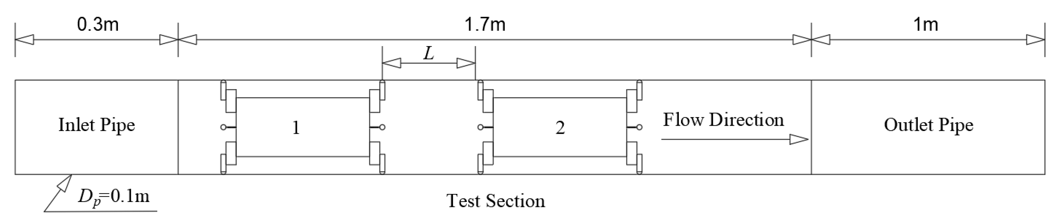
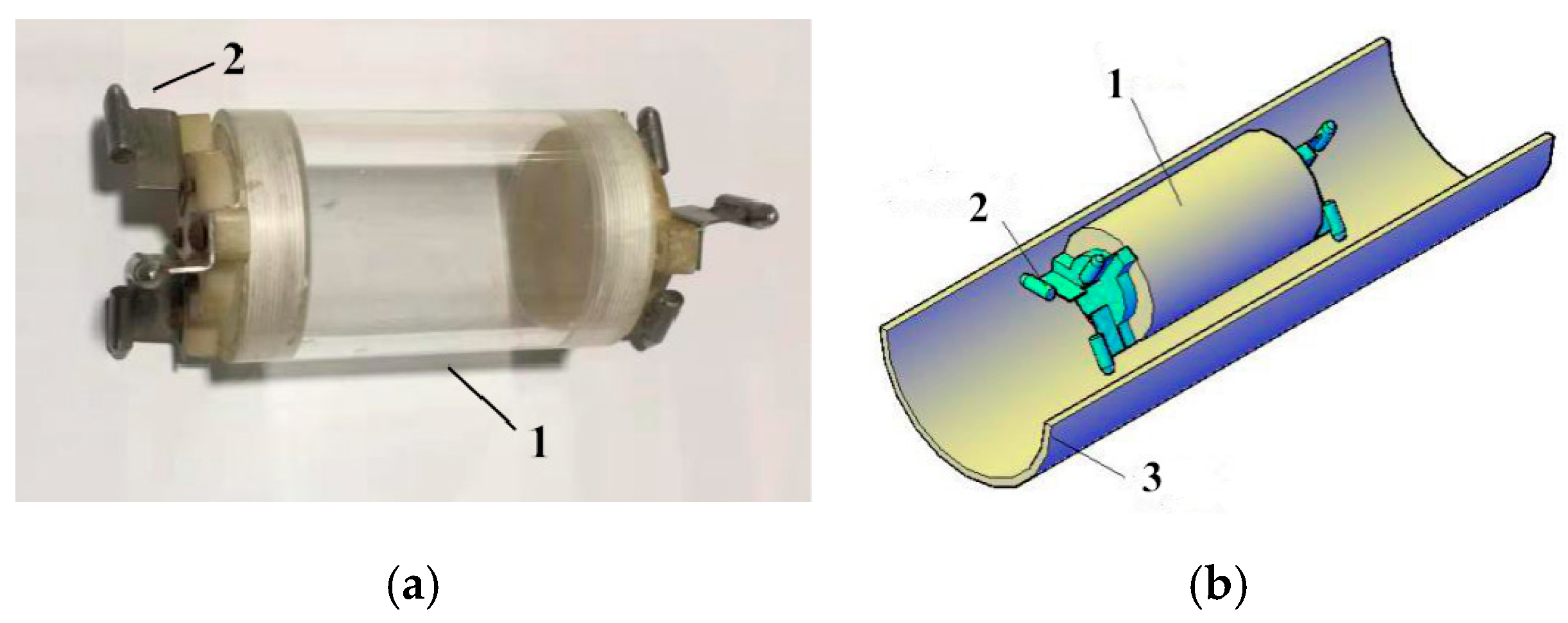
2.1. Geometric Model

The geometric models of pipes and pipe vehicles were created using the commercial software Auto CAD 2014 and were imported into a commercial ICEM CFD package called ANSYS-Fluent. In order to improve the accuracy of the calculation results, the geometric model was simplified slightly to keep it consistent with the original model during the modeling process. The horizontal pipe length was 3 m and the radius Dp was 0.1 m. The geometric model comprised three sections: an inlet pipe, a test section and an outlet pipe with lengths of 0.3 m, 1.7 m and 1 m, respectively, as shown in Figure 1. In order to reduce the influence of the pipe vehicle on the speed entrance cross-section, the length of the inlet pipe was set to 0.3 m. The test section was set to 1.7 m mainly considering the wake influence range and the spacing between the two-pipe vehicles. The outlet section was set to 1 m mainly to reduce the pressure effect of the two-pipe vehicles on the outlet cross-section.
As the core component of the simulation, the pipe vehicle was mainly composed of a barrel and some support bodies, as shown in Figure 2. The barrel was used to contain materials and was made of cylindrical plexiglass of the same material as the pipeline. The diameter Dc of the pipe vehicle was 0.07 m and the length l of the pipe vehicle was 0.15 m. There were six support bodies at the front and rear end of the pipe vehicle positioned every 120°. Each support body was composed of a metal plate and a cylinder. The metal plate had a length of 0.02 m, a height of 0.01 m and a thickness of 0.005 m. The diameter of the cylinder was 0.01 m and the height was 0.002 m. The support body kept the pipe vehicle and the pipeline concentric, avoided the collision of the pipe vehicle and the pipeline and prolonged the use of the pipeline.

2.2. Governing Equations and Turbulence Model
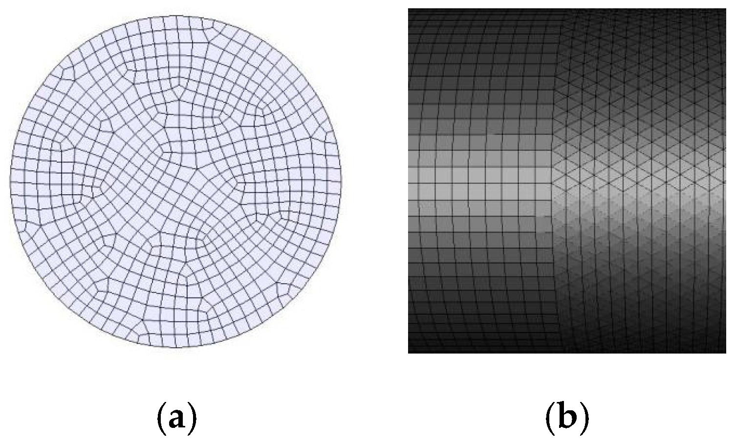
The flow field in the pipeline becomes quite complicated due to the influence of the pipe vehicle structure. Therefore, the simulation process must satisfy the following assumptions: (1) the physical parameters of the water flow must be constant and changes in fluid density must be ignored, and (2) the heat transfer caused by friction between the pipe vehicle and the water flow must be negligible. When the fixing device is released, the pipeline double car starts under the action of water pressure. The continuity equation and the Reynolds time-averaged N–S equation were used in the solving process. In the Cartesian coordinates, the continuity equation and the Reynolds time-averaged equation for the incompressible viscous fluid in the form of a tensor index were written as follows [39,40,41,42]:
ρ t + x i ( ρ u i ) = 0
t ( ρ u i ) + x j ( ρ u i u j ) = p x i + x j ( μ u i x j ρ u i u j ¯ ) + S i
where ρ is the water density; ui and uj are the components of the time-averaged velocity in the i and j directions, respectively; xi and xj are the coordinate components in the i and j directions, respectively; ui′ and uj′ are the fluctuating velocity in the i and j directions, respectively; i and j were 1, 2, and 3, respectively; p is the pressure; μ is the dynamic viscosity; and Si is the projection value of the generalized source term of the momentum equation in the i direction.
The pipe flow through the piped carriage was a fully developed turbulence, and the Reynolds number was more than 4000. Compared with the standard k-ε turbulent model, the RNG k-ε turbulent model can deal better with multiple complicated flow problems such as swirling flow, high strain rate flow and sharply curved streamline flow. The relevant equations can be expressed as follows [43]:
( ρ k ) t + ( ρ k u i ) x i = x j [ α k μ e f f k x j ] + G k + ρ ε
( ρ ε ) t + ( ρ ε u i ) x i = x j [ α ε μ e f f ε x j ] + C 1 ε ε k G k C 2 ε ρ ε 2 k
μ e f f = μ + μ t
μ t = ρ C μ k 2 ε
C 1 ε = C 1 ε - η ( 1 - η / η 0 ) 1 + β η 3
η = ( 2 E i j E i j ) 1 2 k ε
E i j = 1 2 ( u i x j + u j x i )
G k = μ t ( u i x j + u j x i ) u i x j
where k is the turbulence kinetic energy; ε is the turbulent dissipation rate; αk and αε are the effective Prandtl numbers for k and ε, respectively, αk = αε = 1.39; μeff is the effective viscosity; μt is turbulent viscosity, Cμ = 0.0845; C1ε and C2ε are the turbulent model coefficients, respectively; Gk is the generation of turbulent kinetic energy due to the average velocity gradients; and η0 and β are constants.
The RNG k~ε turbulent model is usually used to calculate fully developed turbulence. However, there was a viscous bottom layer near the wall regions, and the flow in the viscous bottom layer was almost laminar, so the RNG k~ε turbulent model was no longer suitable for these regions. The wall function method was used to solve this problem at the pipe wall and the pipe vehicle wall. In order to establish the wall function, two dimensionless parameters, u+ and y+, were used to represent the velocity and distance, respectively. The parameter y+ was the main parameter of the mesh scale in the boundary layer areas of the near-wall areas, which was the dimensionless ratio of the product of both the distance from the wall and the frictional velocity to the dynamic viscosity, which reflected the fineness of the meshes as a whole. The parameters can be calculated by Equations (11) and (12). According to the calculation formula of the boundary layer [16], the number of layers for the boundary layer was set to 11, the thickness of the first layer grid was set to 0.2537 mm (y+ = 30) and the scale factor between layers was set to 1.2.
u + = v p v τ
y + = ρ Δ y v τ η
where ρ is the water density, η is dynamic viscosity, vp is the average velocity of water flow, vτ is the wall friction velocity and ∆y is the distance from the wall.

2.3. Mesh

The commercial ICEM CFD software was used to complete the meshing of the computing domain. The model created by Auto CAD software caused cracks on the surface after importing ICEM CFD; therefore, the geometric model needed to be repaired after importing the ICEM CFD. The geometry repair ensured that the model represented a closed geometry and that there are were extra points or line segments on each surface. The meshing density directly affects the calculation accuracy and calculation time: when the meshing density is large, the calculation time is relatively short but the calculation accuracy is low; if the meshing density is small, the calculation accuracy is high, but a long calculation time is required. Thus, it is necessary to independently test the meshing density. The inlet pipe and outlet pipe were meshed in a hexahedral, unstructured way. The test sections were meshed in a tetrahedral unstructured way due to the relatively complicated structure of the pipe vehicle. The three regions had the same grid size. In order to determine the grid size, taking the two-pipe vehicles with a spacing of 0.5 l as an example, the grids with sizes of 0.005 m, 0.004 m, 0.003 m, 0.002 m and 0.001 m were numerically simulated. The average velocity of water flow at a distance of 0.2 m from the entrance of the pipeline was used as the main reference; the results are shown in Figure 3.
It can be seen from Figure 3 that, as the grid size decreases, the relative error between the simulated velocity values gradually decreases. When the grid size was between 0.001 m and 0.002 m, the relative error between the simulation results was 0.1%. When the grid size was less than 0.002 m, the influence of the grid size on the simulation results was negligible. It was found that when the grid size was 0.002 m, the maximum relative error of the average flow velocity of the cross-section did not exceed 4.3% by comparing the simulation results with the physical experiment results. Considering the actual size of the pipe vehicle, the calculation time and the accuracy of the numerical simulation, the mesh size of the fluid domain was selected to be 0.002 m. Part of the fluid domain meshing is shown in Figure 4.

2.4. Boundary Conditions and Algorithms

The numerical simulation boundary conditions included three parts: the pipeline inlet boundary, pipeline outlet boundary and wall boundary. The three boundary conditions were as follows.
  • The pipeline inlet boundary was set as the “velocity inlet” condition. The liquid medium in the pipeline was water, and the density was 1000 kg/m3 with a dynamic viscosity of 1.062 × 10⁻³ Pa·s (water temperature was 18 °C). The measured velocity was used in order to define the distributions of the flow velocity at the inlet cross-section. The parameters of the “velocity inlet” were calculated by Equations (13)–(17), and the specific calculation results are shown in Table 1.
    Re = ρ V p D p η
    l 0 = 0.07 D P
    I = 0.16 Re - 0 . 125
    k = 1.5 × ( V P × I ) 2
    ε = C μ 0.75 k 1.5 l 0
    where ρ is the water density; η is dynamic viscosity; l0 is turbulence length; I represents turbulence intensity; k is the turbulent kinetic energy; ε is the turbulent dissipation rate; Cμ is the empirical constant of the turbulent model, generally taking 0.09; Vp is the average flow velocity in the pipeline; and Dp is the pipe diameter.
  • The outlet boundary was set as a “pressure outlet” condition. The measured pressure was used to define the pressure distributions at the outlet boundary of the mathematical model. The outlet pressure value was obtained through physical experiment; the pressure was set to 6000 Pa.
  • The wall boundary included the wall surface of the two-pipe vehicles and the pipeline wall, which was set as a “no-slip” condition. The pipeline wall and two-pipe vehicle wall were considered to be hydrodynamically smooth, with a wall roughness constant of zero.
Because the SIMPLEC algorithm has the advantages of high accuracy, good stability and relatively fast calculation speed, we used the algorithm for the pressure and speed coupling in this simulation. For convection terms, we used a second-order difference scheme, momentum equations, turbulent kinetic energy equations and turbulent dissipation rate equations, all of which adopted a second-order upwind style. All convergence accuracies were set to 0.0001.

3. Experimental Methods

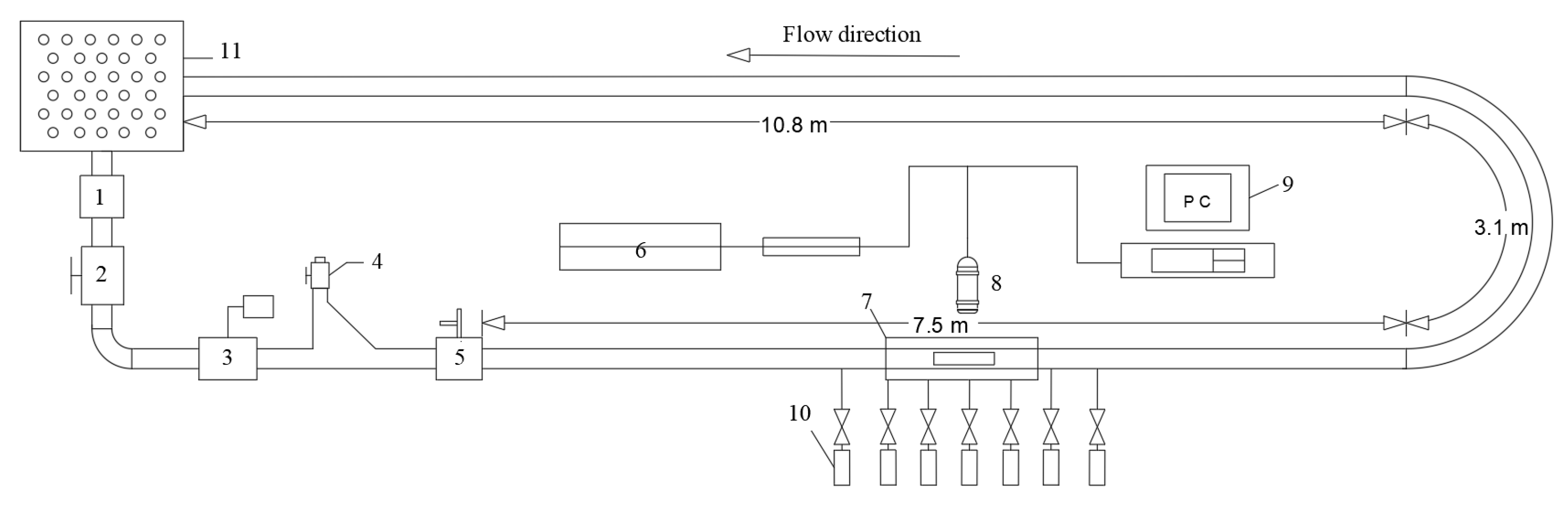
3.1. Experimental System and Procedures

In order to ensure the reliability of the numerical simulation results, a corresponding physical experiment was performed to verify the accuracy of the simulation. The experiment system is shown in Figure 5. The experiment system mainly included three parts: the power system, regulation system and test system. The power system mainly comprised a centrifugal pump; the rated power of the centrifugal pump motor was 15 kw at 2900 r·min−1. The water tank was connected to the centrifugal pump by a steel penstock. The size of the water tank was 1.0 m × 1.0 m × 1.5 m. The regulation system included an electromagnetic flowmeter and a regulating valve. The electromagnetic flowmeter had an accuracy of ±0.5% and a rated pressure of 0.6~4.0 MPa. The test system included a laser Doppler velocimeter and pressure sensors. The pipeline had a total length of 28.6 m and was composed of transparent plexiglas with an inner diameter of 100 mm. The bottom of the pipeline was fixed by brackets so that the entire pipeline was on the same level.
The two-pipe vehicles were defined as the rear and front pipe vehicles in order along the direction of the water flow, as shown in Figure 6. Because the pipeline was made of cylindrical transparent plexiglass, in order to avoid the refraction of laser light by the pipe wall during the test, a rectangular water jacket was installed in the test pipe section. We fixed the two-pipe vehicles to the test pipe section before the experiment began. We filled the water tank with water and added tracer ions to form a complete circuit. Then, the water in the water tank was pumped into the pipeline by a centrifugal pump, and the flow rate was observed by an electromagnetic flowmeter. When the water flow in the pipeline was stable, we measured the water flow velocity and pressure in the pipeline. In order to keep the water temperature constant during the test, the water temperature in the water tank was monitored. When the temperature in the water tank changed, we refilled or changed the water to keep the temperature constant. It was also found that the change in water temperature was relatively small during the test.
The laser Doppler velocimeter (LDV) could realize the non-contact measurement of the flow field, and the measurement error was less than 0.2%, ensuring the accuracy of the test results. During the testing program, the flow was seeded with polystyrene with an average particle size of 6 µm to increase the data collection rate for the LDV. The coordinates of each measuring point were input into the computer, and the laser probe was moved to the corresponding measuring point position for measurement by using the coordinate frame. The processor control target efficiency was 55% with a medium signal-to-noise ratio. The laser flow meter sampled 2000 times per second and made multiple measurements to obtain the average value. The frequency and real-time speed of the measuring points were calculated by the program built in to the software and displayed intuitively on the computer screen. The pressure sensors were linked to a standard dynamic pressure collection system (TST5103, Chengdu Test, Chengdu, China) to measure piezometric heads along the pipelines.

3.2. Experiment Plan

The length and diameter of the pipe vehicle used in the experiment were 150 mm and 70 mm, and the spacing between the two-pipe vehicles was 0.5 l/l/1.5 l/2 l/2.5 l/3 l/4 l, where l represents the length of a single pipe vehicle. The simulated Reynolds number was 115,513, and the corresponding flow Q of the physical experiment was 30 m3/h. The specific experiment scheme is shown in Table 2.

3.3. Section Selection and Measuring Point Arrangement

In order to measure the flow velocity in the annular gap and the flow velocity in the two-pipe vehicle spacing, the corresponding test cross-sections were arranged. Three cross-sections were arranged at equal distances along the direction of each pipe vehicle body. There were five cross-sections arranged in the two-pipe vehicle spacing, two of which were closer to the support body cross-section, and the remaining three cross-sections were arranged at equal intervals. The test sections were numbered along the direction of water flow, in order from 1# to 11#, as shown in Figure 7. In order to measure the three-dimensional flow velocity, a corresponding coordinate system was established in the pipeline; the water flow direction was the Z-axis and the vertical gravity direction was the Y-axis. The corresponding X-axis was established according to the right-hand rule, as shown in Figure 7.
For the annular gap flow field, five measuring rings were arranged, and the measuring ring radii were r1 = rc + 1/5d, r2 = rc + 2/5d, r3 = rc + 1/2d, r4 = rc + 3/5d, r4 = rc + 4/5d (rc is the radius of the pipe vehicle and d is the width of the annular gap); the intersection of the pipe radius and the measuring ring was the layout measuring point, with a total of 60 measuring points, as shown in Figure 8a. For the flow field in the two-pipe vehicles, five measuring rings were also arranged. The outermost two measuring rings’ radii were r5 = rc + 4/5d and r4 = rc + 3/5d. The remaining three measuring rings were distributed at equal intervals; the ring radii were r1′ = 9.5 mm, r2′ = 19 mm and r3 = 28.5 mm. The intersection of the pipe radius and the measuring ring was the arranged measuring point. There were 61 measuring points (including the pipe center point), as shown in Figure 8b.

4. Simulation Results and Discussion

4.1. Distribution of Velocity Magnitude

Figure 9 shows the water flow velocity distribution on the YZ plane at different vehicle spacings. It can be seen that the distribution of the water velocity along the positive direction of the Z-axis at different vehicle spacings was roughly the same. On the left side of the rear pipe vehicle, the water flow distribution in the pipeline was relatively uniform and the velocity value was low. When the water reached the entrance of the annular gap of the rear pipe vehicle, the water flow velocity suddenly increased, and it changed most severely at this cross-section. This was mainly because the area of the cross-section of the annular gap was much smaller than the area of the pipe. According to the continuity equation A1v1 = A2v2, it can be determined that when the area of the cross-section decreased, the flow velocity increased, meaning that the water flow velocity suddenly increased when it entered the annular gap. When the water flow entered the annular gap from the pipeline, the cross-section shrank, and the water flow was compressed, which led it to bend and made the water flow distribution at this position relatively disordered. The entrance of the annular gap was closer to the support body, and the support body therefore also had a certain disturbance effect on the nearby water flow, which further changed the water flow velocity distribution. After the water flowed into the annular gap, the water flow gradually stabilized due to the restriction of the wall of the pipe vehicle and the wall of the pipeline; the streamline also became parallel to the axis of the pipeline and the flow velocity value decreased. When the water flow reached the outlet of the annular gap, the water flow pattern changed drastically again due to the influence of the outlet cross-section and the support body. The presence of the front pipe vehicle further affected the water flow distribution in this section and made the flow pattern more turbulent. The change of velocity in the right annular gap was about the same as that on the left. Figure 10 is a cloud diagram of the velocity distribution of a stationary single-pipe vehicle in the pipeline. It can be seen that the velocity distribution in the annular gap formed by a single-pipe vehicle and two-pipe vehicles was approximately the same by comparing Figure 9 and Figure 10; i.e., with the increase of the number of pipe vehicles, the distribution law of the velocity in the annular gap did not change significantly.
It can also be seen from Figure 9 and Figure 10 that the distribution of the wake area front pipe vehicle and the wake area of a single pipeline vehicle were approximately the same; that is, the rear pipe vehicle has no significant impact on the wake area of front pipe vehicles under different vehicle spacings. The wake area of the rear pipe vehicle (the spacing part of the two-pipe vehicles) changed as the spacing between the vehicles changed. When the vehicle spacings were 0.5 l and l, the water flow velocity from the center of the pipe along the pipe diameter direction showed a trend of decreasing first, then increasing and finally decreasing. This was mainly because a backflow region was formed after the water flowed out of the annular gap. When the two-pipe vehicles were closer, the hindering effect of the right pipe vehicle on the backflow region was strong, which restricted the development of the backflow region, which could not spread downstream, and so the backflow region filled the entire two-pipe vehicle spacing. The flow velocity value in the backflow region showed a decreasing trend from the center of the pipe to the pipe wall. In the outer region of the backflow region, part of the water flowing out of the annular gap continued to move forward at high speed due to inertia, and the flow velocity value of this part was larger than that of the backflow region. The flow velocity value gradually decreased due to the existence of viscous resistance in the vicinity of the pipe wall. When the two-pipe vehicle spacing was greater than l, the obstruction of the right pipe vehicle to the backflow region gradually weakened as the spacing increased, the backflow region spread downstream and developed, and the flow velocity value at the center of the pipeline gradually decreased during the diffusion process. At a certain spacing from the left pipe vehicle, the flow velocity from the center of the pipe to the pipe wall showed a trend of increasing first and then decreasing. When the two-pipe vehicle spacing was further expanded to 3 l, the right pipe vehicle had almost no effect on the flow field in the two-pipe vehicle spacing, and the flow field distribution of the rear pipe vehicle and the front pipe vehicle was roughly the same. When the distance between the two vehicles in the pipeline reached 4 l, the flow field distribution in the spacing was no longer affected by the two-pipe vehicles. In comparison to the flow field distribution of a single pipe vehicle, it was found that the velocity distribution of the front and rear pipe vehicle was the same as that of a single pipe vehicle; that is, when the vehicle spacing was greater than 4 l, the interaction between the two-pipe vehicles could be ignored.
When water flowed through the support body, a cylindrical flow phenomenon was formed, resulting in more complicated changes in the flow field distribution of the cross-section where the support body was located. The velocity distribution of the cross-section of the two-pipe vehicle support body at 0.5 l, l and 2 l was taken as an example for analysis, and the velocity distribution cloud map is shown in Figure 11. The four support body cross-sections were numbered along the direction of the water flow; these are cross-sections 12#, 13#, 14# and 15# in order.
It can be seen from Figure 11 that the flow velocity distribution of cross-sections 12#, 13# and 15# was approximately the same under different pipe vehicle spacings; that is, the flow velocity along the center of the pipeline toward the pipe wall showed a trend of increasing first and then decreasing. It can also be seen from the figure that the overall velocity distribution of cross-sections 12#, 13# and 15# showed small changes under different pipe vehicle spacings, while the change at cross-section 14# was relatively large. This was mainly due to the different blocking strength of the right pipe vehicle to the water flow when the vehicle spacing was different. When the distance between the two-pipe vehicles was small, after the water flowed out of the left annular gap, it was quickly “blocked” by cross-section 14#, so the velocity distribution changed sharply. With the increasing distance between the two-pipe vehicles, the water flowing out of the left annular gap was blocked by cross-section 14# after flowing forward for a certain distance. The redistribution of the water flow before contacting cross-section 14# was more stable than when it flowed out of the annular gap, so the change of velocity distribution at this cross-section was also relatively mild. With the increasing distance between two-pipe vehicles, the velocity distribution of cross-section 14# gradually changed to cross-section 12#. The water flow in the pipeline was evenly distributed and the flow velocity was low before contacting cross-section 12#, so the change of the flow velocity at this cross-section was relatively small. Cross-sections 13# and 15# were located at the exit of the annular gap, and there was a backflow region near the two cross-sections, which made the flow velocity of the two cross-sections change drastically.

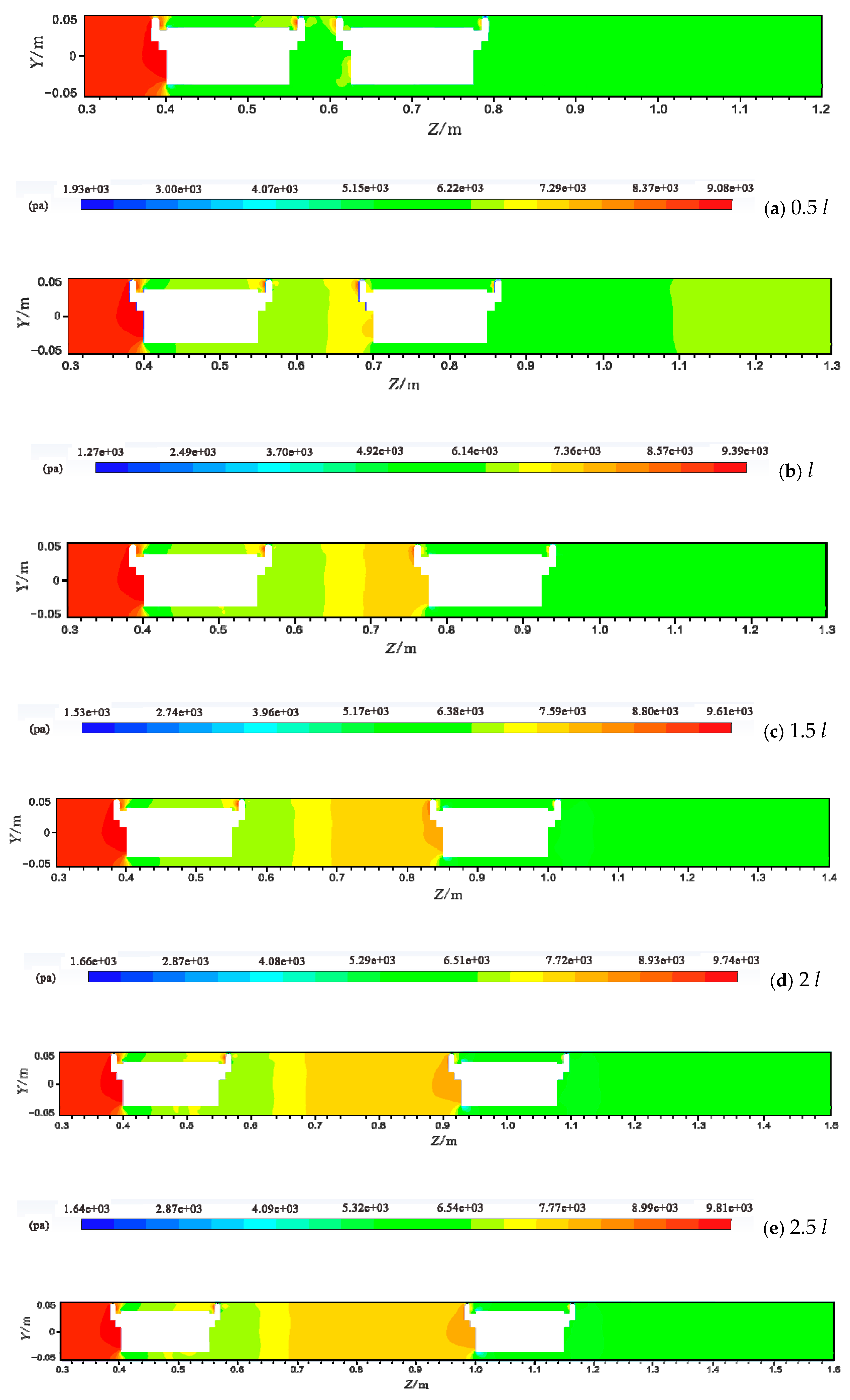
4.2. Distribution of Pressure

Figure 12 shows the pressure distribution on the YZ plane at different vehicle spacings. It can be seen from Figure 12 that the pressure distribution in the pipeline can be divided into four regions: the pipeline inlet region, the annular gap region, the two-pipe vehicle spacing region and the pipeline exit region.
(1)
The pipeline inlet region was from the pipeline entrance to the left annular gap entrance, and the pressure showed a trend of decreasing first and then increasing. This was mainly due to the fact that the average water velocity in the pipeline was almost the same before the water flow contacted the left pipe vehicle. According to the energy equation, when the kinetic energy and potential energy were unchanged, the pressure energy was reduced due to the existence of the drag loss along the path, so the pressure value was reduced accordingly. When the water flow approached the pipe vehicle, the water flow velocity blocked by the pipe vehicle decreased rapidly and part of the kinetic energy was converted into pressure energy, so the pressure increased.
(2)
In the left annular gap region, the pressure along the positive direction of the Z-axis showed a trend of first decreasing and then increasing, but in the right annular gap, the pressure value gradually decreased. This was mainly because the water flow was blocked by the end face of the pipe vehicle at the entrance of the annular gap, so the pressure value was high. Constrained by the annular gap, the velocity of the water flow in the annular gap was relatively stable; that is, the kinetic energy change was relatively small. However, due to the influence of the viscous resistance near the pipe vehicle wall and the pipeline wall, the total energy of the water flow was reduced, meaning that the pressure energy was reduced, and the pressure gradually decreased. The blocking effect of the right pipe vehicle affected the pressure field near the exit of the left annular gap, and the pressure value at the exit of the left annular gap therefore increased. However, the water flowing out of the right annular gap was no longer blocked by obstacles, and so there was no pressure increase at the outlet of the right annular gap.
(3)
In the two-pipe vehicle spacing region, the pressure change was small when the two-pipe vehicles spacing was 0.5 l. With the increase of the vehicle spacing, the pressure in the two-pipe vehicles spacing showed a gradually increasing trend along the positive direction of the Z-axis. According to the above analysis, it can be determined that the change of the water flow velocity in the spacing was small when the distance between the two-pipe vehicles was 0.5 l, the change in kinetic energy was relatively small, and the change in pressure energy was also small, and so the pressure change in the two-pipe vehicle was small. When the vehicle spacing was greater than 0.5 l, the water flow velocity gradually decreased along the positive direction of the Z-axis due to the blocking effect of the right-hand pipe vehicle, the kinetic energy was gradually converted into pressure energy and the pressure gradually increased. Therefore, the pressure in the workshop gradually increased along the positive direction of the Z-axis.
(4)
The pipeline exit region was from the right annular gap exit to the pipeline outlet, and the pressure showed a trend of increasing first and then decreasing along the positive direction of the Z-axis. This was mainly due to the flow of water from the right annular gap forming a high-speed backflow region near the end face of the pipe vehicle. The backflow region had a higher water flow velocity, so the kinetic energy was larger and the pressure energy was correspondingly lower. The backflow region expanded downstream and the water flow velocity decreased, so the kinetic energy decreased and the corresponding pressure energy increased. When it was sufficiently far away from the right pipe vehicle, the water flow gradually stabilized and the velocity value remained unchanged; that is, the kinetic energy remained unchanged, but the simultaneous loss of resistance gradually reduced the pressure energy, and so the pressure decreased accordingly.
Figure 13 presents a cloud diagram of the pressure distribution in the pipeline when a single pipe vehicle is stationary. By comparing Figure 12 and Figure 13, it was found that, similar to the change in water flow, the change in the number of pipe vehicles did not affect the pressure distribution in the pipeline inlet region, the right annular gap and the pipeline outlet region, but only changed the magnitude of the pressure; the pressure value in the pipeline inlet region increases the most. When the number of pipe vehicle increased, the pressure value in the pipeline also increased. This was mainly because, with the increase in the number of pipe vehicles, the water flow was hindered by the pipe vehicles, which increased the pressure value in the pipeline.
The main driving force of the pipe vehicle originates from the pressure difference between the front and rear ends. The magnitude of the pressure difference will also have an impact on the starting acceleration and transport speed of the pipe vehicle and ultimately affect the transportation efficiency of the pipe vehicle. The change in pressure difference between the front and rear pipe vehicles under different spacings is shown in Figure 14.
It can be seen from Figure 14 that the change rule of the pressure difference between the front and rear pipe vehicles is roughly the same; that is, as the vehicle spacing increases, the pressure difference decreases first and then increases and finally gradually stabilizes. This was mainly because when the vehicle spacing was less than 1.5 l, the flow field between the two-pipe vehicles changed drastically and the energy loss was large. When the kinetic energy of the water flow was approximately unchanged, the pressure energy decreased accordingly, resulting in a lower pressure difference between the front and rear pipe vehicles. With the gradual increase of the spacing between the two-pipe vehicles, the changes in the flow field of the vehicle spacing gradually flattened, the energy loss decreased and the pressure energy increased accordingly, thereby increasing the pressure difference of the front and rear pipe vehicles. According to the starting acceleration formula of the pipe vehicle (Equation (18)), when the diameter, length and load of the pipe vehicle were unchanged, the starting acceleration of the two-pipe vehicles was proportional to the pressure difference between the front and rear pipe vehicles. Therefore, as the vehicle spacing increased, the starting acceleration of the two-pipe vehicles also increased. It can also be seen from Figure 14 that the pressure difference between the front pipe vehicle and the rear pipe vehicle became smaller than that of only one pipe vehicle in the pipeline; that is, the starting acceleration obtained by a single-pipe vehicle was greater than that of two-pipe vehicles. This conclusion was also verified through model tests. This provides a certain reference for the selection of a suitable spacing between the two-pipe vehicles.
a = F p + F τ - f m = Δ P · A c + π D c l τ - μ ( G F g ) m
where Fp is the differential pressure, f is the frictional force, Fτ is the shear force on the surface of the two-pipe vehicles, τ is the shear stress on the wall of the pipe vehicle, G is the total gravity of the pipe vehicle under load, µ is the dynamic friction factor, and Fg is the buoyancy of the two-pipe vehicles.

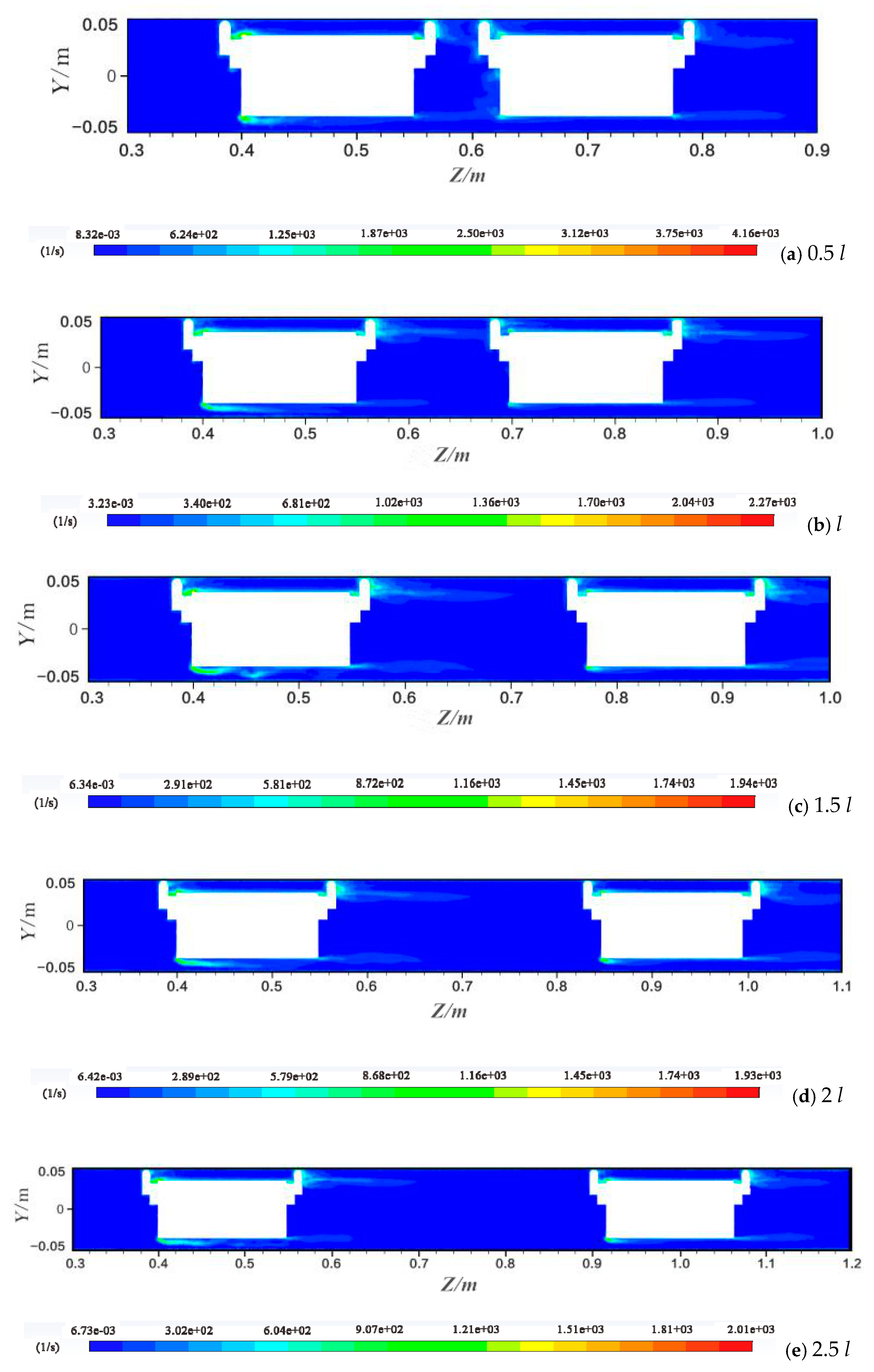
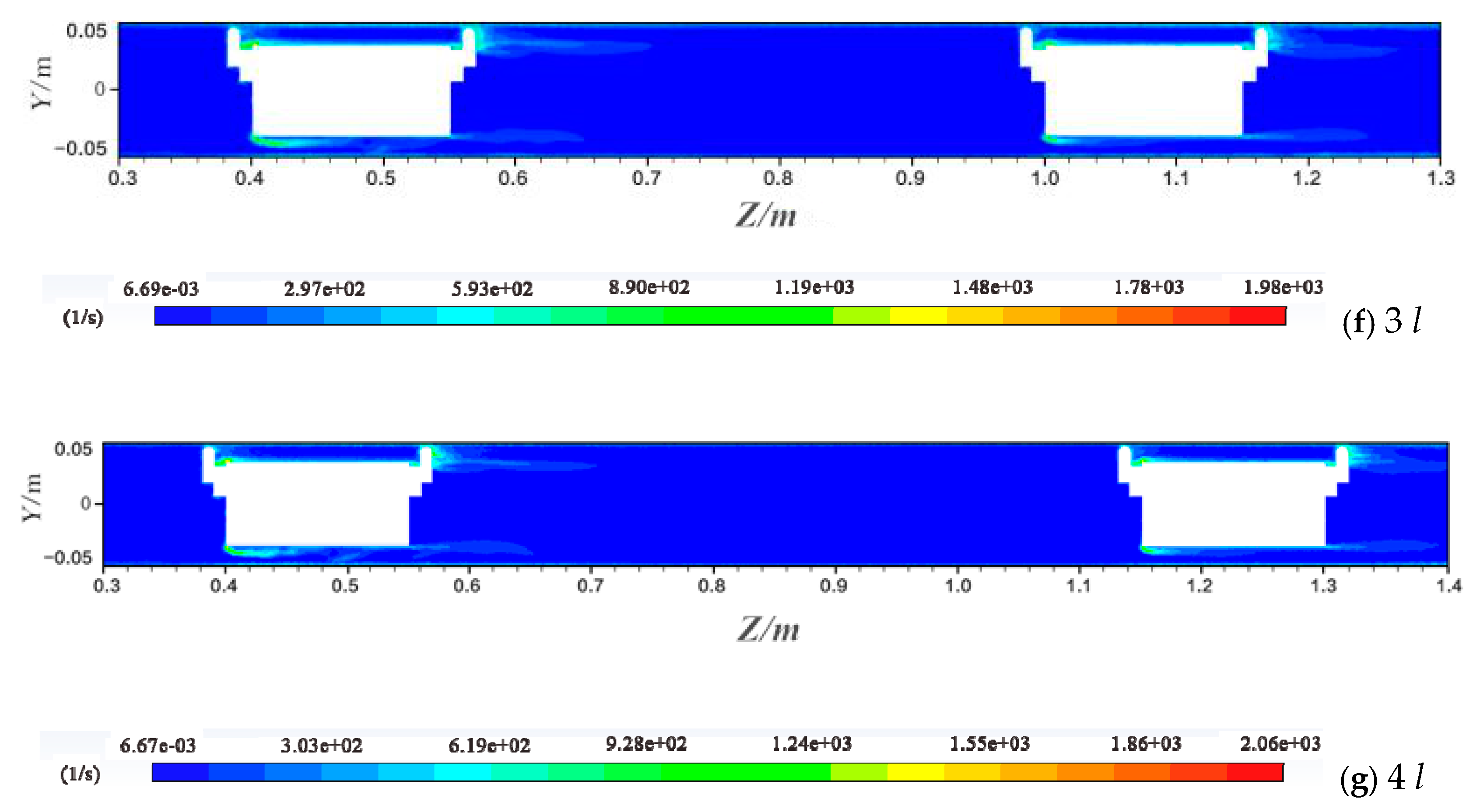
4.3. Distribution of Vorticity

Since the barrel and the support body were both cylindrical, the pipe vehicle could be regarded as a spatial multi-cylinder assembly. A vortex was created when water passed through the pipe vehicle. The generation and disappearance of vortices were accompanied by the loss and dissipation of energy. Therefore, the analysis of the vorticity characteristics generated by the two pipe vehicles at different spacings has a certain guiding significance for improving the structure of pipe vehicles and for reducing energy consumption.
Figure 15 shows the cloud map of the vorticity distribution of the two-pipe vehicles at different spacings. It can be seen from the figure that the flow of the tandem two-pipe vehicles did not have a vortex shedding phenomenon as with the traditional flow around the cylinder. The vorticity value was large near the support body and the entrance and exit of the annular gap. This was because vortices were generated when water flowed through the support body; a vortex also occurred at the entrance and exit of the annular gap under the influence of the end face of the pipe vehicle. The distance between the support body and the annular gap was relatively short, and the vortices generated in these places were mixed with each other, meaning that the vorticity value increased. When the vortex diffused into the annular gap, the development of the vortex was restricted by the pipe vehicle wall and the pipe wall, the vortex gradually disappeared after spreading in the annular gap for a distance and no vortex was observed in the posterior half of the annular gap. Constrained by the end face of the pipe vehicle, the water velocity in the spacing between the two-pipe vehicles was low and relatively stable, meaning that there were no vortices. In order to more accurately represent the change of vorticity near the support body, the cross-section of the support body of the two-pipe vehicles with a spacing of 1.5 l is taken as an example for analysis, as shown in Figure 16.
It can be seen from Figure 16 that regions with large vorticity values mostly appear near the surface of the support body. The vorticity value of cross-sections 12# and 14# (near the entrance of the annular gap) was smaller than that of cross-sections 13# and 15# (near the exit of the annular gap). This was mainly due to the boundary layer separation and vortices generated when the water flowed around the support bodies near the entrance of the annular gap. The vortices were driven to diffuse downstream by the water flow, making the vorticity value at cross-sections 12# and 14# smaller. When the water flowed out of the annular gap, boundary layer separation occurred again under the influence of the end face of the pipe vehicle, and the generated vortices spread to cross-sections 13# and 15#, mixing with the vortices generated at these two sections, meaning that the vorticity values at cross-sections 13# and 15# increased. It can be seen that by further simplifying the support structure and optimizing the cross-section structure of the pipe vehicle, the generation of vortices can be reduced and the energy consumption loss can be reduced.

5. Verification of the Simulated Results

5.1. Velocity Distribution

Taking the water velocity values at cross-sections 2#, 6# and 10# with spacings of 0.5 l/1.5 l/3 l as an example, the results of the physical experiment and numerical simulation were compared and analyzed, as shown in Figure 17.
Figure 17 shows the comparison between the experiment value and the numerical simulation value of each section under different vehicle spacings. The experimental values are in good agreement with the numerical simulation values, and the maximum relative error does not exceed 8.47%. When the two-pipe vehicles spacings were different, the change of the annular gap flow along the pipe radial was the same; that is, the annular gap flow velocity value along the direction of the pipe vehicle wall to the pipe wall showed a trend of increasing first and then decreasing. This was mainly due to the existence of viscous forces near the pipe vehicle wall and the pipe wall, so the water flow velocity was low. At a distance from the pipe vehicle wall and the pipe wall, the annular gap flow velocity value gradually increased. It can also be seen that the flow velocity changes in the annular gap between the left vehicle and the right vehicle were the same; that is, the velocity change in the annular gap between the two-pipe vehicles was not affected by the vehicle spacing. Both the numerical simulation and the experiment show that the maximum flow velocity in the spacing appears near the wall of the pipeline, which was different from the flow velocity at the center of the pipeline when the pipe is full, indicating that the existence of the two-pipe vehicles has an impact on the flow field distribution. When the vehicle spacing was small, the flow velocity of the spacing would first decrease, then increase and then decrease as the distance from the center of the pipeline increased. When the vehicle spacing was 3 l, the flow velocity of the spacing increased first and then decreased as the distance from the center of the pipeline increased. The water flow velocity distribution of the vehicle spacing along the pipe radius was consistent with the previous analysis.
The annular gap velocity formula in the YZ plane was fitted according to the experimental data, as shown in Table 3 and Table 4.
Table 3 and Table 4 show that the velocity distribution in the annular gap was a quadratic parabola, but the water flow was distributed logarithmically when the pipe was full. It can also be seen from Figure 17 that the flow field distribution in the vehicle spacing was also different from that when the pipe was full, which indicates that the presence of two pipe vehicles will change the flow velocity distribution pattern in the pipeline.

5.2. Pressure Distribution

Figure 18 shows a comparison between the experimental value and the numerical simulation value of the average pressure of each cross-section. The relative error between the experiment value and the numerical simulation value did not exceed 8%. The experimental results showed that the pressure distribution changes in the annular gap under different vehicle intervals were roughly the same. The pressure value in the left annular gap decreased first and then increased along the positive direction of the Z-axis, while the pressure value in the right annular gap gradually decreased along the positive direction of the Z-axis. The pressure in the spacing gradually increased along the positive direction of the Z-axis, and the pressure reached the maximum near the right annular gap. The average pressure value of each cross-section in the right annular gap was smaller than that of the left annular gap at different vehicle spacings. The water flow had a large energy loss when it reached the right annular gap, meaning that the total energy of the water flow in the right annular gap was lower than that on the left. Because the velocity values in the left and right annular gaps were about the same—that is, the kinetic energy was the same—the average pressure value of each section in the annular gap on the right was small.

6. Conclusions

In this article, the characteristics of the flow field of a two-pipe vehicle under different vehicle spacings were studied by a combination of numerical simulation and physical experiment. The maximum relative error between the numerical simulation result and the physical experiment value did not exceed 9%, which proves that the method of studying the two-pipe vehicle system by numerical simulation is feasible. The main research conclusions are summarized as follows:
  • Compared with a single-pipe vehicle, the water flow and pressure change rules of the pipeline inlet region, annular gap region and the pipeline outlet region of the two-pipe vehicles are the same. With the increase of the number of pipe vehicles, the change of the water flow velocity value is relatively small, and the change of the internal pressure value of the pipeline is large. This provides a certain reference for future research on the changes of water flow and pressure distribution when multiple vehicles are stationary in the pipeline.
  • Under different vehicle spacing conditions, the velocity of the annular gap along the direction of water flow shows a trend of increasing first, then decreasing and finally increasing; from the pipe vehicle wall to the pipe wall, the water flow velocity shows an increase and then a decrease. As the vehicle spacing gradually increases, the flow field in the spacing is gradually weakened by the influence of the two-pipe vehicles. When the vehicle spacing reaches 4 l, the interaction between the two-pipe vehicles is negligible.
  • The pressure changes in the pipeline along the water flow direction are approximately the same under different vehicle spacing conditions. In the pipeline inlet region, the pressure gradually decreases along with the pipe vehicle. In the annular gap of the rear pipe vehicle, the pressure shows a trend of decreasing first and then increasing, but in the annular gap of the front pipe vehicle, the pressure showed a gradually decreasing trend. When the vehicle spacing is 0.5 l, the pressure change in the spacing is small. As the vehicle spacing gradually increases, the pressure appears to gradually increase along the direction of the water flow. In the pipeline outlet region, the pressure shows a trend of increasing first and then decreasing.
  • As the vehicle spacing increases, the pressure difference decreases first and then increases and finally gradually stabilizes. The change law of the starting acceleration of the two-pipe vehicles under different vehicle spacings is consistent with the change law of pressure difference.
  • The vorticity value is large near the entrance and exit of the annular gap and around the support bodies, and there is no vortex shedding in the pipeline under different vehicle spacings. The generation and dissipation of vortices can be reduced by simplifying the support body structure and optimizing the shape of the end face of the pipe vehicle.
The study of the characteristics of the flow field under different vehicle spacings in this paper provides a certain theoretical reference for the selection of suitable two-pipe vehicle spacings. This will lay the foundation for further research into the starting speed and energy consumption loss of two-pipe vehicles. At the same time, the research in this paper also enriches the theory of annular gap flow and provides technical support for the continuous improvement of HCP technology.

Author Contributions

X.J. designed the experimental schemes and purchased the experimental materials; X.S. provided the experimental sites and the necessary experimental equipment; X.S. and Y.L. reviewed the manuscript and provided the technical guidance on the research subject; X.J. wrote and revised the manuscript and completed the numerical calculation. All authors have read and agreed to the published version of the manuscript.

Funding

The research was funded by the National Natural Science Foundation of China (51179116, 51109155, 50579044, 51705352) and the Natural Science Foundation of Shanxi Province (2015011067, 201701D221137).

Acknowledgments

The research was supported by the Collaborative Innovation Center of New Technology of Water-Saving and Secure and Efficient Operation of Long-Distance Water Transfer Project at Taiyuan University of Technology.

Conflicts of Interest

The authors declare no conflicts of interest.

References

  1. Hodgson, G.W.; Charles, M.E. The pipeline flow of capsules. Can. J. Chem. Eng. 1963, 42, 43–45. [Google Scholar]
  2. Kruyer, J.; Redberger, P.G.; Ellis, H.S. The pipeline flow of capsules. J. Fluid Mech. 1967, 30, 513–531. [Google Scholar] [CrossRef]
  3. Brown, R.A.S. Capsule pipeline research at the Alberta Research Council, 1985–1978. J. Pipeline 1987, 6, 75–82. [Google Scholar]
  4. Charles, M.E. Theoretical analysis of the concentric flow of cylindrical forms. Can. J. Chem. Eng. 1963, 41, 46–51. [Google Scholar]
  5. Ellis, H.S. An experimental investigation of the transport by water of single cylindrical and spherical capsules with density equal to that of the water. Can. J. Chem. Eng. 1964, 42, 1–8. [Google Scholar] [CrossRef]
  6. Van den Kroonenberg, H.H. A Mathematical Model for Concentric Horizontal Capsule Transport. Can. J. Chem. Eng. 1978, 56, 538–543. [Google Scholar] [CrossRef] [Green Version]
  7. Latto, B.; Chow, K.W. Hydrodynamic transport of cylindrical capsules in a vertical pipeline. Can. J. Chem. Eng. 1982, 60, 713–722. [Google Scholar] [CrossRef]
  8. Liu, H.; Graze, H.R. Lift and drag on stationary capsule in pipeline. J. Hydraul. Eng. 1983, 109, 28–47. [Google Scholar] [CrossRef]
  9. Liu, H.; Noble, J.S.; Wu, J.; Zuniga, R. Economics of coal log pipeline for transporting coal. Transp. Res. 1998, 32, 377–391. [Google Scholar] [CrossRef]
  10. Liu, H.; Wu, J.P. Economic Feasibility of Using Hydraulic Pipeline to Transport Grain in the Midwest of the United States; Freight Pipeline (Proc. 6th Int. Symp, on Freight Pipelines); Hemisphere Publishing Corp: New York, NY, USA, 1990; pp. 135–140. [Google Scholar]
  11. Liu, H.; Richards, J. Hydraulics of stationary capsule in pipe. J. Hydraul. Eng. 1994, 120, 22–40. [Google Scholar] [CrossRef]
  12. Tomita, Y.; Yamamoto, M.; Funatsu, K. Motion of a single capsule in a hydraulic pipeline. J. Fluid Mech. 1986, 171, 495–508. [Google Scholar] [CrossRef]
  13. Lenau, C.W.; El-Bayya, M.M. Unsteady flow in hydraulic capsule pipeline. J. Fluid Eng. 1996, 122, 1168–1173. [Google Scholar] [CrossRef]
  14. Vlasak, P. An experimental investigation of capsules of anomalous shape conveyed by liquid in a pipe. Powder Technol. 1999, 104, 207–213. [Google Scholar] [CrossRef]
  15. Quadrio, M.; Luchini, P. Direct numerical simulation of the turbulent flow in a pipe with annular cross section. Eur. J. Mech. 2002, 21, 413–427. [Google Scholar] [CrossRef]
  16. Mohamed, F.; Khalil, S.Z.; Kassab, I.G. Turbulent flow around single concentric long capsule in a pipe. Appl. Math. Model 2009, 34, 2000–2017. [Google Scholar]
  17. Asim, T.; Mishra, R. Computational fluid dynamics based optimal design of hydraulic capsule pipelines transporting cylindrical capsules. Powder Technol. 2016, 295, 180–201. [Google Scholar] [CrossRef] [Green Version]
  18. Asim, T.; Mishra, R. Development of a design methodology for hydraulic pipelines carrying rectangular capsules. Int. J. Press. Ves. Pip. 2016, 146, 111–128. [Google Scholar] [CrossRef] [Green Version]
  19. Asim, T.; Mishra, R. Optimal design of hydraulic capsule pipeline transporting spherical capsules. Can. J. Chem. Eng. 2016, 94, 966–979. [Google Scholar] [CrossRef]
  20. Zhang, X.L.; Sun, X.H.; Li, Y.Y. 3-D numerical investigation of the wall-bounded concentric annulus flow around a cylindrical body with a special array of cylinders. J. Hydrodyn. 2015, 27, 120–130. [Google Scholar] [CrossRef]
  21. Sun, X.H.; Li, Y.Y.; Yan, Q.F. Experimental study on starting conditions of the hydraulic transportation on the piped carriage. In Proceedings of the 20th National Conference on Hydrodynamics, Taiyuan, China, 23–25 August 2007; pp. 425–431. [Google Scholar]
  22. Wang, R.; Sun, X.H.; Li, Y.Y. Transportation characteristics of piped carriage with different Reynolds numbers. J. Drain Irrig. Mach. Eng. 2011, 29, 343–346. [Google Scholar]
  23. Li, Y.Y.; Sun, X.H. Mathematical model of the piped vehicle motion in piped hydraulic transportation of tube-contained raw material. Math. Probl. Eng. 2019, 2019, 1023–1033. [Google Scholar] [CrossRef]
  24. Wang, J.; Sun, X.H.; Li, Y.Y. Analysis of pressure characteristics of tube-contained raw material pipeline hydraulic transportation under different discharges. In Proceedings of the International Conference on Electrical, Mechanical and Industrial Engineering (ICEMIE), Phuket, Thailand, 24–25 April 2016; pp. 44–46. [Google Scholar]
  25. Li, Y.Y.; Sun, X.H.; Yan, Y.X. Hydraulic characteristics of tube-contained raw material hydraulic transportation under different loads on the piped carriage. Trans. Chin. Soc. Agric. Mach. 2008, 39, 93–96. [Google Scholar]
  26. Jing, Y.H. Characteristics of Slit Flow Velocity by the Formation of Stable Moving Piped Carriage with Different Diameter in Straight Piped Segments. Master’s Thesis, Taiyuan University of Technology, Taiyuan, China, 2014. [Google Scholar]
  27. Yang, X.N. Study on the Character of Spiral Flow Caused by Different Length Guide Vanes. Master’s Thesis, Taiyuan University of Technology, Taiyuan, China, 2013. [Google Scholar]
  28. Zhang, C.J.; Sun, X.H.; Li, Y.Y. Effects of Guide Vane Placement Angle on Hydraulic Characteristics of Flow Field and Optimal Design of Hydraulic Capsule Pipelines. Water 2018, 10, 1378. [Google Scholar] [CrossRef] [Green Version]
  29. Lu, Y.F. Research on the Numerical Simulation of the Velocity of the Concentric Annular Gap Spiral Flow around the Stationary Column in the Horizontal Straight Pipeline. Master’s Thesis, Taiyuan University of Technology, Taiyuan, China, 2018. [Google Scholar]
  30. Zhang, X.L.; Sun, X.H.; Li, Y.Y.; Xi, X.N.; Guo, F.; Zheng, L.J. Numerical investigation of the concentric annulus flow around a cylindrical body with contrasted effecting factors. J. Hydrodyn. 2015, 27, 273–285. [Google Scholar] [CrossRef]
  31. Li, Y.Y.; Sun, X.H.; Xu, F. Numerical simulation on the piped hydraulic transportation of tube-contained raw material based on FLOW-3D. Syst. Eng.-Theory Pract. 2013, 33, 262–266. [Google Scholar]
  32. Feng, J.; Huang, P.Y.; Joseph, D.D. Dynamic simulation of the motion of capsules in pipelines. J. Fluid Mech. 1995, 286, 201–227. [Google Scholar] [CrossRef]
  33. Zhang, C.J.; Sun, X.H.; Li, Y.Y.; Zhang, X.L.; Zhang, X.Q.; Yang, X.N.; Li, F. Hydraulic Characteristics of Transporting a Piped Carriage in a Horizontal Pipe Based on the Bidirectional Fluid-Structure Interaction. Math. Probl. Eng. 2018, 2018, 43–60. [Google Scholar] [CrossRef]
  34. Bearman, P.W.; Wadcock, A.J. The interaction between a pair ofcircular cylinders normal to a stream. J. Fluids Struct. 1973, 61, 499–511. [Google Scholar]
  35. Zdravkovich, M.M. The effects of interference between circular cylinders in cross flow. J. Fluids Struct. 1987, 1, 239–261. [Google Scholar] [CrossRef]
  36. Cui, W.Z.; Zhang, X.T.; Li, Z.X.; Li, H.; Liu, Y. Three-dimensional numerical simulation of flow around combined pier based on detached eddy simulation at high Reynolds numbers. Int. J. Heat Technol. 2017, 35, 91–96. [Google Scholar] [CrossRef]
  37. Alam, M.M. Lift Forces Induced by the Phase Lag Between the Vortex Sheddings from Two Tandem Bluff Bodies. J. Fluid Struct. 2016, 65, 217–237. [Google Scholar] [CrossRef]
  38. Carmo, B.S.; Meneghini, J.R. Numerical investigation of the flow around two circular cylinders in tandem. J. Fluid Struct. 2006, 22, 979–988. [Google Scholar] [CrossRef]
  39. Rahimi, H.; Schepers, J.G.; Shen, W.Z.; Ramos García, N.; Schneider, M.S.; Micallef, D.; Simao Ferreira, C.J.; Jost, E.; Klein, L.; Herráez, I. Evaluation of different methods for determining the angle of attack on wind turbine blades with CFD results under axial inflow conditions. Renew. Energy 2018, 125, 866–876. [Google Scholar] [CrossRef] [Green Version]
  40. Magdalena, T.; Jarosław, B. The Impact of the Strength of Roof Rocks on the Extent of the Zone with a High Risk of Spontaneous Coal Combustion for Fully Powered Longwalls Ventilated with the Y-Type System—A Case Study. Appl. Sci. 2019, 9, 53152019. [Google Scholar]
  41. Magdalena, T.; Jarosław, B. Analysis of the Impact of Auxiliary Ventilation Equipment on the Distribution and Concentration of Methane in the Tailgate. Energies 2018, 11, 3076. [Google Scholar]
  42. Wojciech, S. The basic equations of fluid mechanics in form characteristic of the finite volume method. Technol. Sci. 2011, 14, 299–313. [Google Scholar]
  43. Yakhot, V.; Orzag, S.A. Renormalization group analysis of turbulence: Basic theory. J. Sci. Comput. 1986, 1, 3–11. [Google Scholar] [CrossRef]
Figure 1. Schematic of horizontal pipe section. Note: 1 and 2 represent the pipe vehicles. L represents the vehicle spacing; the value of L in this simulation is 0.5 l/l/1.5 l/2 l/2.5 l/3 l/4 l.
Water 12 02158 g001
Figure 2. Schematic of pipe vehicle. (a) The physical model of the pipe vehicle; (b) The geometric model of the pipe vehicle. Note: 1. Barrel. 2. Support body. 3. Pipeline.
Water 12 02158 g002
Figure 3. Schematic diagram of grid independence test. Note: v represents the average velocity of water flow at a distance of 0.2 m from the entrance of the pipeline.
Water 12 02158 g003
Figure 4. Schematic of mesh generation: (a) Meshing of inlet pipe and outlet pipe; (b) Meshing of connected sections.
Water 12 02158 g004
Figure 5. Experimental system. Note: 1. Centrifugal pump. 2. Regulating valve. 3. Electromagnetic flowmeter. 4. Feeding device. 5. Brake device. 6. Laser Doppler velocimeter. 7. Rectangular water jacket. 8. Laser probe. 9. Computer. 10. Pressure sensors. 11. Water tank.
Water 12 02158 g005
Figure 6. Experimental equipment and instruments. Note: 1. Rear pipe vehicle. 2. Front pipe vehicle. 3. Rectangular water jacket. 4. Coordinate frame. 5. Laser probe. 6. Pressure sensors.
Water 12 02158 g006
Figure 7. The layout of measuring cross-sections. Note: 1. Rear pipe vehicle. 2. Front pipe vehicle. L represents the two-pipe vehicle spacing. 1#~11# represent the measuring cross-sections.
Water 12 02158 g007
Figure 8. Schematic of measuring point layout. (a) Arrangement of measuring points in the annular gap. (b) Arrangement of measuring points in the vehicle spacing. Note: r1~r5 are the radii of the measuring rings in the annular gap; r1′~r5′ are the radio of the measuring rings in the vehicle spacing.
Water 12 02158 g008
Figure 9. Velocity magnitude distribution cloud map of the YZ plane under different vehicle spacings. (a) L = 0.5 l. (b) L = l. (c) L = 1.5 l. (d) L = 2 l. (e) L = 2.5 l. (f) L = 3 l. (g) L = 4 l.
Water 12 02158 g009aWater 12 02158 g009b
Figure 10. Velocity magnitude distribution cloud map of a single pipe vehicle in the YZ plane.
Water 12 02158 g010
Figure 11. The velocity magnitude distribution cloud map of the support body cross-sections at different vehicle spacings. (a) L = 0.5 l. (b) L = l. (c) L = 2 l. Note: 12# and 13# represent the cross-section of the support body of the left pipe vehicle; 14# and 15# represent the cross-section of the support body of the right pipe vehicle.
Water 12 02158 g011aWater 12 02158 g011b
Figure 12. The pressure distribution cloud map of the YZ plane under different vehicle spacings. (a) L = 0.5 l. (b) L = l. (c) L = 1.5 l. (d) L = 2 l. (e) L = 2.5 l. (f) L = 3 l. (g) L = 4 l.
Water 12 02158 g012aWater 12 02158 g012b
Figure 13. The pressure distribution cloud map of a single pipe vehicle in the YZ plane.
Water 12 02158 g013
Figure 14. Pressure difference between front and rear pipe vehicles under different spacings.
Water 12 02158 g014
Figure 15. Vortex distribution cloud map of the YZ plane under different vehicle spacings. (a) L = 0.5 l. (b) L = l. (c) L = 1.5 l. (d) L = 2 l. (e) L = 2.5 l. (f) L = 3 l. (g) L = 4 l.
Water 12 02158 g015aWater 12 02158 g015b
Figure 16. Vortex magnitude distribution cloud map of the support body cross-sections with 0.5l vehicle spacings. (a) Vorticity at 12# section. (b) Vorticity at 13# section. (c) Vorticity at 14# section. (d) Vorticity at 15# section. Note: 12# and 13# represent the cross-section of the support body of the left pipe vehicle; 14# and 15# represent the cross-section of the support body of the right pipe vehicle.
Water 12 02158 g016
Figure 17. Comparison of experimental value and numerical simulation value on the velocity magnitude. (a) L = 0.5 l. (b) L = 1.5 l. (c) L = 3 l. Note: 2# represents the middle cross-section of the left pipe vehicle, 6# represents the cross-section in the middle of the spacing and 10# represents the middle cross-section of the right pipe vehicle.
Water 12 02158 g017
Figure 18. Comparison of experimental values and numerical simulation values of the average pressure. (ac) The comparison between the numerical simulation values and the experimental values with vehicle spacings of 0.5 l/1.5 l/3 l.
Water 12 02158 g018
Table 1. The parameter values of the pipeline liquid.
Velocity Inlet (m/s)Rek (m2/s2)ε (m2/s3)Il0 (m)
1.03115,5130.0024 0.0028 0.03780.007
Table 2. Experiment plan.
Rear Pipe Vehicle
l (mm) × Dc (mm)
Front Pipe Vehicle
l (mm) × Dc (mm)
Q
(m3/h)
L
(mm)
Condition
150 × 70150 × 70300.5 l/l/1.5 l/2 l/2.5 l/3 l/4 lStatic
Note: L represents the two-pipe vehicle spacing; Q represents the flow; l represents the length of the pipe vehicle; Dc represents the diameter of the pipe vehicle.
Table 3. Fitting formula of the annular gap flow velocity of the rear pipe vehicle.
L (mm)Fitting FormulaR2
0.5 lZ = −0.0316Y2 + 2.7482Y57.470.9458
1.5 lZ = −0.0133Y2 + 1.509Y22.6010.9211
3 lZ = −0.0073Y2 + 0.6558Y12.940.9823
Note: L represents the two-pipe vehicle spacing; R2 represents correlation coefficient.
Table 4. Fitting formula of the annular gap flow velocity of the front pipe vehicle.
L (mm)Fitting FormulaR2
0.5 lZ = −0.008Y2 + 0.6942Y13.0390.9552
1.5 lZ = −0.0094Y2 + 0.8295Y16.1790.9947
3 lZ =0.009Y2 + 0.7957Y15.380.9791
Note: L represents the two-pipe vehicle spacing; R2 represents correlation coefficient.

