A Method to Improve the Flood Maps Forecasted by On-Line Use of 1D Model

Abstract

Forecasting floods in urban areas during a heavy rainfall is the aim of every early warning system. 2D-models produce the most accurate flood maps, but they are practically useless as quasi real-time tools, because their run times are comparable to times of propagation of floods. Run times of 1D-model are of tens of seconds, but their predictions lack accuracy and many useful indicators of flood severity. Our aim is the identification of the 2D-model map that is more similar to the actual map, chosen among those simulated off-line. To this aim, we produce a rough flood map of the occurring event, through a quasi real-time simulation of the rainfall-runoff using a 1D-model. Then we apply an original method, named “ranking approach”, to perform the best matching. This method is applied to the Corace torrent (Calabria, Southern Italy), using 17 synthetic hyetographs to simulate the same number of rainfall-runoff events, using 1D (Storm Water Management Model) and 2D (Danish Hydraulic Institute, 1995) models. The method proves to be effective in 65% of the cases, while in 82% of cases (i.e., for 14 cases out 17), the event produced by the same ietograph falls within the third rank.

1. Introduction

Flooding is one of the most frequent natural disasters [1]. The effects of flooding are particularly severe in urban areas [2], where lost of life and heavy damage to infrastructures can be associated with the most hazardous flood events. Urban flooding is usually due to the filling and failure of the stormwater collection and drainage systems [3]. The management of stormwater in urban areas is a complex task, since it depends on a large number of natural (e.g., the temporal and spatial variability of precipitation and the hydrological response of the soil) and human (e.g., the extent of urban areas and the size and type of drainage systems) factors. An accurate prediction of stormwater is important for an efficient analysis and safe planning of drainage systems in urban or peri-urban watersheds [4]. In this regards, a reliable and efficient flood model is useful to predict the extent of inundation, water depths, discharge partition and flow velocity in urbanized flood prone areas [5,6]. The use of hydraulic and hydrological models provides system managers information about how the drainage system will respond to the most intense precipitations [7] and support planning and operation of early flood warning systems [8]. To this goal, many hydrologic computer models were developed to study watershed hydrology with applications in rural and urban areas [9,10]. Several flood models, such as HEC-RAS [11], TUFLOW [12], CSIRO TVD [13], AutoRAPID [14], and HAND [15], are not suitable for urban flood simulations under heavy precipitation because of their inappropriateness in reflecting the spatial and temporal dynamics of urban flooding process [16]. The use of hydrological models has become a common practice in agro-forest areas, although the accuracy of the model predictions largely depends on the quality of hydrological and geomorphological input data [17]. By contrast, flood prediction in urban areas is more complicated and time-consuming. As a matter of fact, the hydrological responses of urban and rural areas to precipitation are different, since they depend on different hydraulic and hydrological processes. Therefore, the models used for urban flood simulations need to account for the specific processes of the urban environment, where the stormwater follows multiple flow paths such as crossroads, sewers and buildings [6,18,19,20]. Prediction of flooding effects can be carried out using several numerical models, which can be categorized into (a) one-dimensional (1D) models, (b) two-dimensional (2D) models, and (c) one-dimensional river flow models coupled with two-dimensional floodplain flow (1D-2D) models [21,22]. The 1D hydrodynamic models are computationally efficient, but they are not able to simulate flow diffusion on a continuous surface; on the contrary, the 2D models offer a high level of accuracy, but are computationally intensive [13]. Generally speaking, the simulation of rainfall-runoff events by 2D models provides reliable estimations of the flood parameters (e.g., the runoff volumes, peak discharge, time, and duration of flood) and maps in urban areas [23,24]. However, in the case of small drained watersheds, flood predictions in real time are not possible using a 2D model, because the computation time (sometimes several hours) can be even higher than the basin’s concentration time (typically a few hours) of the smallest watersheds [25,26,27]. This problem makes the setup of early-warning alert systems, based on reliable weather predictions (for instance, using meteorological radar) practically impossible. These systems must provide not only the flood water depths and maps, but also the time when the flood will peak, which is a fundamental parameter to warn the population of flood hazards [28]. Combining the quickness of computation procedures of 1D models and the prediction accuracy of 2D models may be a possible solution to provide reliable flood maps in real time when heavy and flash precipitation approaches urban areas located in small watersheds. Some examples of urban flood predictions in urban areas coupling 1D and 2D models were reported. In a small urbanized area in West Bengal (India), Storm Water Management Model (SWMM) and MIKE URBAN models were used to simulate flood extent and inundation from daily annual maximum rainfall [29]. Different types of hydraulic–hydrodynamic models (the 1D HEC-RAS and MIKE 11 models, the 2D MIKE 21 and MIKE 21 FM models as well as the 1D-2D coupled hydraulic models MIKE 11/MIKE 21 within the MIKE FLOOD platform), applied in the lower part of the Xerias River (Volos, Greece), indicated the sensitivity of floodplain modelling on the digital elevation model (DEM) spatial resolution and the hydraulic modelling approach [30]. In the same environment (a small urban catchment in the center of Athens, Greece), the surface and sewer system were coupled by [31], using MIKE URBAN and MIKE FLOOD, showing the higher feasibility of 1D-2D coupled models in simulating flood extent and inundation in urban areas, compared to a 1D model (SWMM). However, few studies (e.g., [32,33], working in watersheds of the humid environment) used a 1D model with computation time of the order of minutes, for flood predictions in real time coupled with a 2D model. However, no modelling studies in peri-urban and small catchments are available in semi-arid environments (such as the Mediterranean Basin). The Mediterranean water courses, characterised by small drainage areas and steep channel profile, are subject to frequent and intense storms. These factors determine flash and hazardous floods in the torrents with possible heavy risks for livings and civil works in urban areas [34,35]. The need for modelling flash flood in peri-urban areas subject to the flood risk in the Mediterranean torrents inspired this study, which proposes a method to produce accurate flood maps in urban areas using the 1D model SWMM [36]. We propose to use SWMM online, which is continuously running embedded in an early warning system, with the aim to foresee any river flood which causes the overflows of the river banks and the inundation of the adjacent low-lying lands. The running strategy is described in Sub-Section 3.3, and it is conceived to run backward (in hindcasting mode), using hyetograph measured by rainfall data and upward (in forecasting mode), using the meteorological radar predictions. During a rainfall event, the model results of the running should predict with an advance of a few hours, the water discharge and volume as well as the area of a possible inundation. Run times are typically of tens of seconds. As said, the accuracy of prediction of 1D-model are severely reduced in comparison to 2D-model map, therefore we will obtain an imprecise inundation map, without information regarding dynamic parameters. Moreover, some critical information to assess the dangerousness of the flooding, e.g., the velocity of inundating water, is completely missing. The original contribution of the paper consists of the methodology exposed in Section 2, aimed at choosing the 2D-model map which has the maximum likelihood with that produced by the occurring event, using the 1D-model as a blurred representation of the latter. This best matching map is chosen among a large numer of maps generated off-line through MIKE URBAN, MOUSE/MIKE11 and MIKE FLOOD (Danish Hydraulic Institute, 1995), using as input synthetic hyetographs. To validate the method, it was applied to an urban area located at the outlet of a small peri-urban watershed of Southern Italy (Corace River, Calabria). Finally, an online early-warning platform for flood forecasting based on the developed method is proposed.

2. Materials and Methods

2.1. Description of the Methods

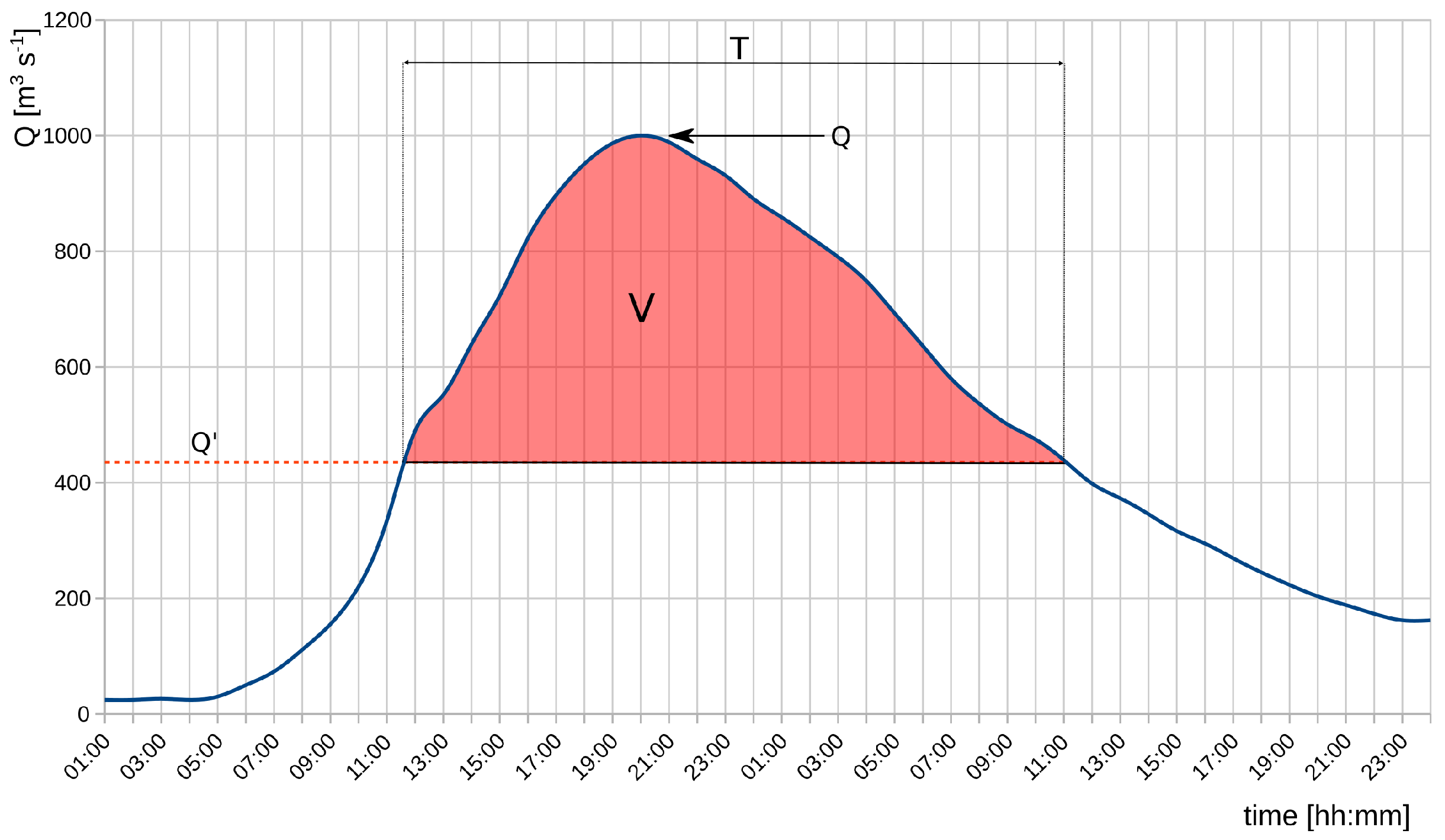
2.1.1. Foreword

In a drainage system an extreme flood may lead to the inability of a river cross section to convey the flood water and thus to the overflow limit (hereinafter indicated by Q’). In a hydrograph of a flood, four important hydraulic variables can be found (Figure 1):

-

the peak flow Q, which is the maximum value of the flow;

-

the flooding time T, that is the time when the Q > Q’;

-

the overflow volume V_f , that is the water volume exceeding the hydraulic capacity of the drainage system;

-

the mean overflow $\overline{Q}$, which is simply the ratio between V and T.

These four variables can be simulated by both 1D, 2D or 1D-2D prediction models.

2.1.2. Modeling of the Hydraulic Parameters

The 1D and 1D-2D models were used to predict the four variables above introduced (V, Q, T and $\overline{Q}$) and to produce the flood maps after a sample of selected hyetographs. To this aim, a catalogue of hyetographs was prepared, varying the precipitation characteristics, such as the hyetograph shape (e.g., Chicago, triangular, rectangular), return interval (e.g., from 2 to 500 years), and rainfall duration (e.g., from 1 to 24 h) and amount (the rainfall depths). The variables V, Q, T and $\overline{Q}$ of flood produced by the synthetic hydrographs were simulated by the 1D model. Then, the 1D simulations were compared to the corresponding simulations given by the 1D-2D model (Figure 2).

The comparison accuracy was checked adopting the main statistics (the mean, standard deviation, maximum and minimum values) and four indexes commonly used in hydrological modeling (e.g., [28,35,37,38,39]): coefficient of determination r², coefficient of efficiency E, Root Mean Square Error RMSE, and Coefficient of Residual Mass CRM. The related equations are reported in the works of Zema et al. [40], Krause et al. [41], Moriasi et al. [42] and Liew V. and Garbrecht [43]. To summarise:

-

r² ranges from 0 (no agreement between model and data variance) to 1 (perfect agreement); values over 0.5 are acceptable for Liew V. and Garbrecht [43], Santhi et al. [44], Vieira et al. [45];

-

E ([46]) is the most common measure of model accuracy and ranges from $-\infty$ to 1; the model accuracy is “good” if E ≥ 0.75, “satisfactory” if 0.36 ⩽ E ⩽ 0.75 and “unsatisfactory” if E ⩽ 0.36 ([43]);

-

RMSE, which measures the average error between observations and predictions, should be as closest as possible to zero [47]; RMSE is considered poor, if its predicted value is higher than 0.5 of the measured standard deviation [48];

-

CRM (also reported as “percent bias (-)”, PBIAS), if positive, indicates model underestimation, whereas, if negative, overestimation [49]; CRM below 25% for runoff is considered fair [42].

Moreover, the V-Q values simulated by the 1D and 1D-2D model for the same events were plotted on a V-Q chart, in order to visually identify the model accuracy.

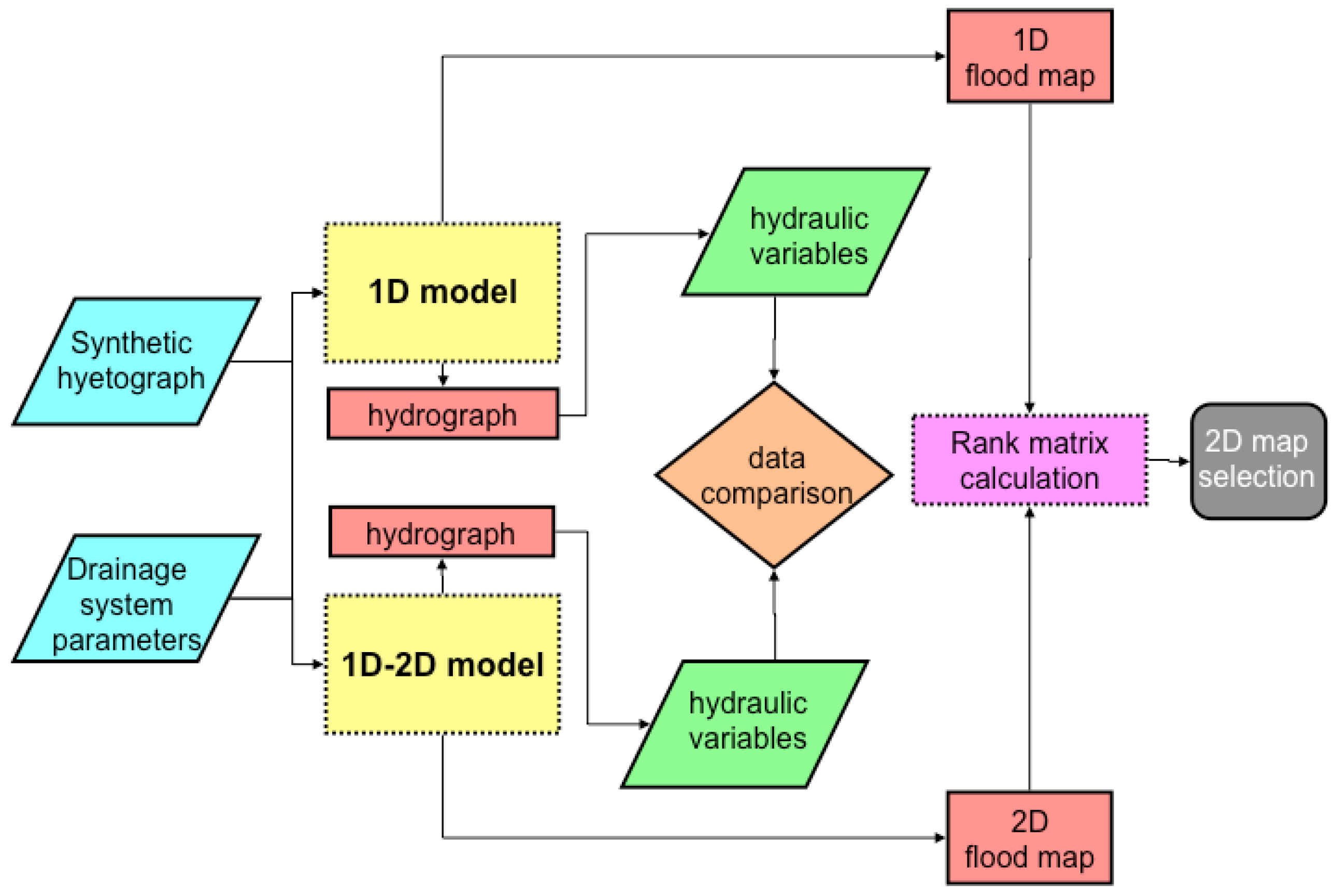
2.1.3. Flood Map Selection

The flood maps consist of the water depths simulated by the 1D or the 1D-2D model using a 1-m grid overlaid on the urban sub-watersheds built on soil topography. Then, the flood map produced by the 1D model is associated with the 2D flood map produced by the same synthetic hyetograph, adopting an approach (henceforth indicated as ranking approach) based on the maximum similarity between the 1D and 2D maps. In this ranking approach, the 1D flood map is associated with the 2D map calculating the rank of a set indicators for the event catalogue. The proposed method is able to select the most similar 1D and 2D flood maps. The method hypothesizes that a flood map, where each point is a flood depth over the urban area, is a geometric figure processed using the area geometry properties. Thus, the 2nd order moments are calculated for both 1D and 2D maps. The following indicators were selected:

-

the flood area A;

-

the flood volume V;

-

the flood depth (mean) D;

-

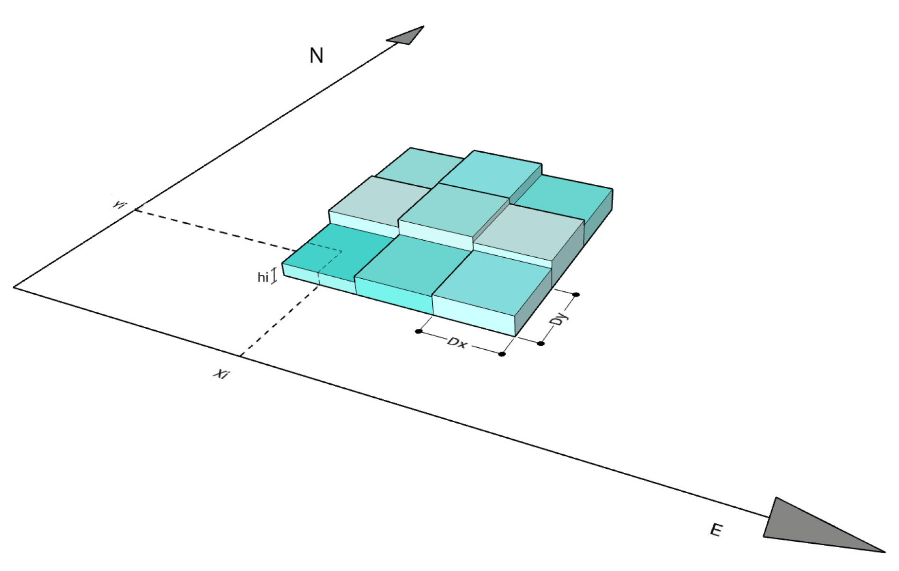
coordinates ($X,Y$) of center of mass, where

$$X={\displaystyle \frac{{\sum }_{i=1}^n{x}_i{h}_i}{{\sum }_{i=1}^n{h}_i}},Y={\displaystyle \frac{{\sum }_{i=1}^n{y}_i{h}_i}{{\sum }_{i=1}^n{h}_i}};$$

(1)

with $n,x_i,y_i$, total number and coordinate north and east of each pixel image, and $h_i$ its depth value (Figure 3);

-

ratio between moment of inertia about the north and east directions (IgN, IgE), where:

$$IgN=\sum _{i=1}^n{x}_i^2{h}_i,IgE=\sum _{i=1}^n{y}_i^2{h}_i;$$

(2)

-

polar moment of inertia, $Io=$ IgN + IgE;

-

centrifugal moment of inertia, $Ic={\sum }_{i=1}^n{x}_i{y}_i{h}_i$;

-

ratio between moment of inertia about north direction and polar moment of inertia ($\frac{IgN}{Io}$)

-

ratio between moment of inertia about east direction and polar moment of inertia ($\frac{IgE}{Io}$);

-

ratio between the difference between moments of inertia about east and north direction and polar moment of inertia ($\frac{IgE-IgN}{Io}$)

-

ratio between centrifugal moment of inertia and polar moment of inertia ($\frac{Ic}{Io}$).

2.1.4. The Similarity Algorithm Based on the “Ranking Approach”

Let $\mathit{D}$ be the matrix of the jth indicator calculated for the map of the ith event produced by the 1D-2D model:

$$\mathit{D}={\left[d_{ij}\right]}_{\begin{array}{c}i=1,\cdots ,m\\ j=1,\cdots ,n\end{array}}\in {\mathbb{R}}^{mxn},$$

(3)

and $\mathit{S}$ the corresponding matrix of indicators for the map produced by the 1D model:

$$\mathit{S}={\left[s_{ij}\right]}_{\begin{array}{c}i=1,\cdots ,m\\ j=1,\cdots ,n\end{array}}\in {\mathbb{R}}^{mxn},$$

(4)

From these matrices it is possible to easily calculate the matrices of ranks ${\mathit{D}}_{\mathit{r}}$ and ${\mathit{S}}_{\mathit{r}}$, where each element ($d{r}_{ij}$ and $s{r}_{ij}$) is the rank of the jth indicator for the event ith, using 2D and 1D maps, respectively. ${\mathit{D}}_{\mathit{r}}$ and ${\mathit{S}}_{\mathit{r}}$, have the following expressions:

$${\mathit{D}}_{\mathit{r}}={\left[d{r}_{ij}\right]}_{\begin{array}{c}i=1,\cdots ,m\\ j=1,\cdots ,n\end{array}}\in {\mathbb{N}}^{mxn}and{\mathit{S}}_{\mathit{r}}={\left[s{r}_{ij}\right]}_{\begin{array}{c}i=1,\cdots ,m\\ j=1,\cdots ,n\end{array}}\in {\mathbb{N}}^{mxn}.$$

(5)

Each row of the matrices ${\mathit{D}}_{\mathit{r}}$ ed ${\mathit{S}}_{\mathit{r}}$ being a map represented by a vector in the space ${\mathbb{N}}^n$, it is possible to calculate the Euclidean distance among vectors. Let $c_{kl}$ is the geometric distance between the k vector $D{r}_k$ and l vector $S{r}_l$:

$$c_{kl}=\sqrt{\sum _{j=1}^m{(d{r}_{kj}-s{r}_{lj})}^2},$$

(6)

the following square matrix is calculated:

$$C={\left[c_{kl}\right]}_{\begin{array}{c}k=1,\cdots ,m\\ l=1,\cdots ,m\end{array}}\in {\mathbb{R}}^{mxn}.$$

(7)

The $C$ matrix is not symmetric; its main diagonal ($k=l$) reports the distance between the vector of the 1D and 2D maps for the same event, respectively. The element on the main diagonal is on of the ranks of $c_{kl}$ ($e_{kl}$) for $k=l$ between the lth map produced by the 1D and the kth map generated by the 2D model. Overall, if $e_{kl}$ is equal to 1 the predicted lth map is best the 1D map, which better fits the kth 2D map of catalogue of flood event considered, while if the rank is equal to 2, the 1D map is the second map, which better fits the 2D map after the 1D map corresponding to the rank = 1, and so on. The ratio between the total number ranks equal to 1 on a column and m is the absolute frequency, the ratio between the total number of 2 and m is the relative frequency of 2 ($f_2$) and the same for the total number of 3 ($f_3$). Of course, $0\le f_p\le 1(p=1,2,3)$.

The cumulative frequency is:

$$F_p=\sum _{i=1}^p{f}_i.$$

(8)

$F_p$, can be considered to be acceptable if higher than 0.8, which means that p predicted maps have an acceptable cumulative frequency, and, on the other hand, one of the p maps is certainly the most similar 1D map to the 2D map generated by the rainfall event considered.

2.1.5. Uncertainty Analysis of the Selected Map

In hydrological modelling, the evaluation of the simulation uncertainty is a critical and meaningful step for an effective real-time forecasting [50,51]. Therefore, we suggest to select the three 2D-model maps indicated by our approach as the closest to the 1D-model map, and to evaluate the percent difference of some meaningful physical variables (i.e., the mean flood depth) between the “expected” 2D-model map and these three maps. Clearly, the “expected” map is the 2D-model map produced by the same hyetograph generating the 1D-model map. For the on-line use of the method, the comparison is made using as “expected map” the actual map, which is known at the end of the event.

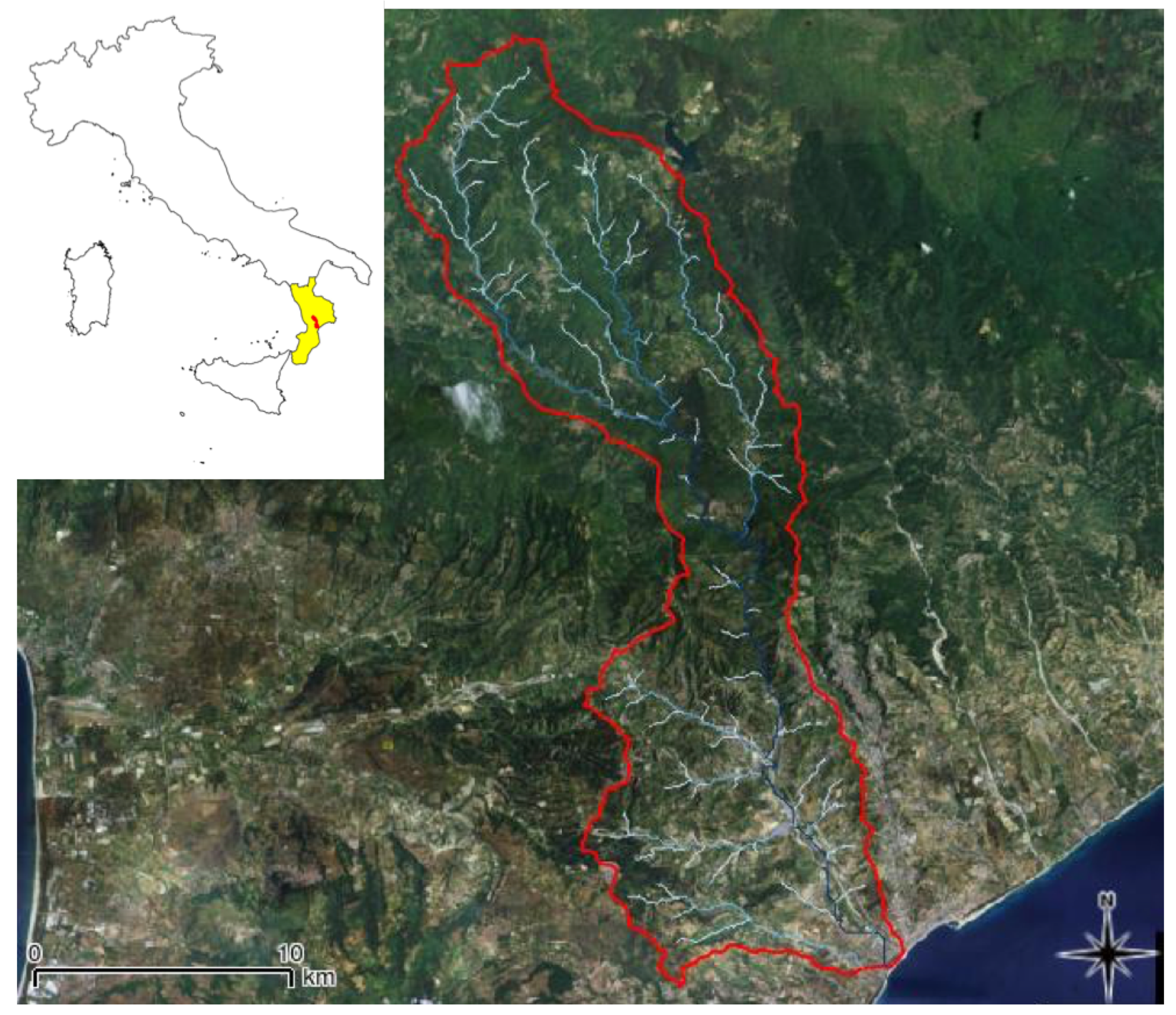
2.2. Method Application to a Case Study (Corace Watershed, Calabria, Southern Italy)

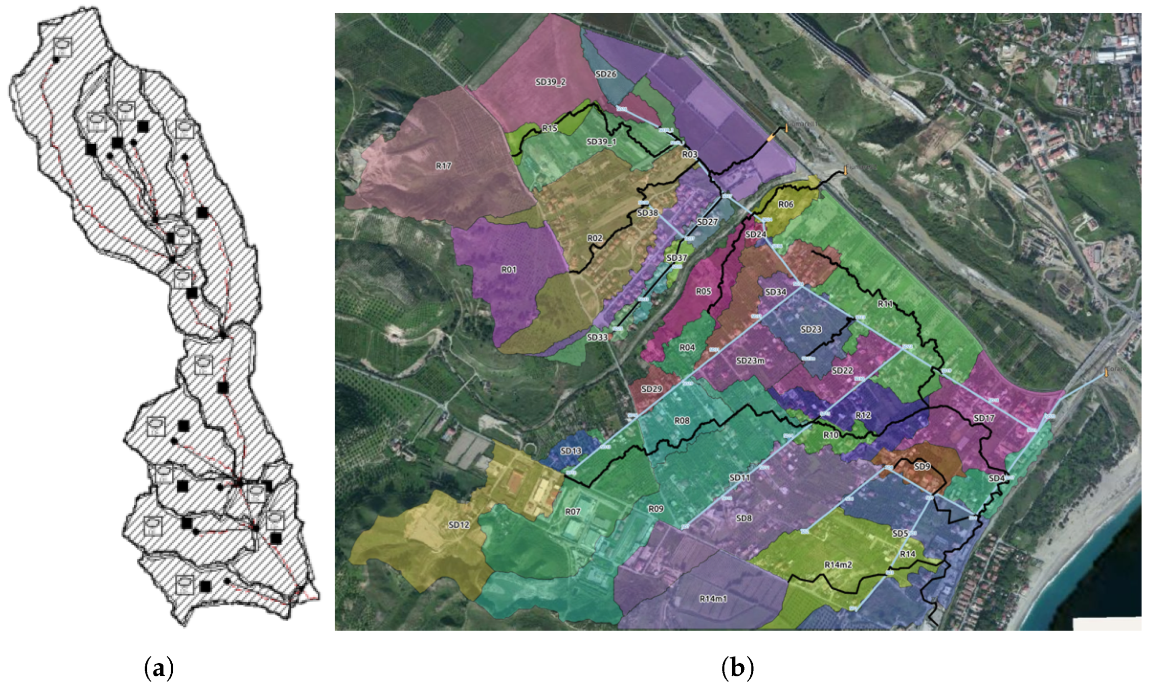
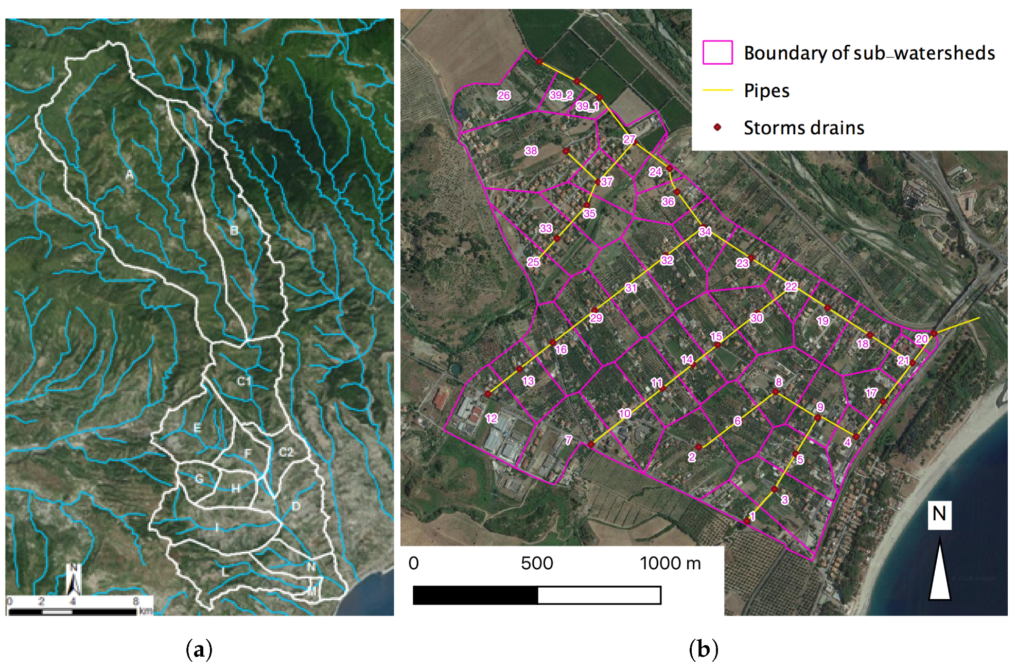
2.2.1. Description of the Study Area

The Corace torrent is a seasonally flowing water course of mid Calabria (Southern Italy) (Figure 4). The watershed covers 294 km², while its perimeter is 113 km. The main stream (53-km long) rises at 1600 m above sea level into the mountain system of ”Serre” (Central Calabria) and flows flows in channels with a mean slope of 2.3% as far into the Ionian Sea near the city of Catanzaro. The watershed has an elongated shape. The concentration time [52], was estimated according to Kirpich [53], and is equal to 7.4 h (

Table 1. Main morphometric parameters of Corace watershed (extracted from the DTM).

Parametres		Measuring Unit	Value
Area		km2	294
Perimeter		km	113
Shape coefficient		-	1.86
Altitude (a.s.l.)	max	m	1385
	mean	m	565
	min	m	1
Drainage density		km/km2	4.32
Length of the main reach		km	53.3
Concentration time		h	7.4
Mean yearly precipitation		mm	1279
Mean yearly temperature		°C	12.9

Note: The morphometric and topographic characteristics of the watershed were drawn from 5-m (for rural areas) and 1-m (for urban areas) DTM built by a laser imaging detection and ranging (LIDAR) survey.

).

The geological units of the studied watershed are mainly composed of granitic gneiss (24% of the total area) and phyllite (23%); other units are porfiroid, marble and green schist. The prevalent land use are represented by forests (52%), located in the upper areas, and agricultural areas (41%), distributed almost homogenously in the watershed; urban zones (2%) in valleys and pasture (5%) cover the remaining areas as reported by the Corine land cover, scale 1:100,000, 2006 [54].

According to the “Soil Map of the Calabria Region” the soils are mainly sandy loamy (60% of sand, 28% of loam and 12% of clay).

The mean annual precipitation is about 1300 mm, while mean temperature is close to 13 $°$C. The urban area, located in the downstream part of the watershed, covers a total area of 341 hectares. The hydraulic network consists of both sub-surface drainage system and surface earth ditches (small to medium size). The surface area was topographically reproduced through a detailed digital terrain model (digital terrain model (DTM)) of both soil contours and urban infrastructures.

2.2.2. Construction of the Hydrological Database

Seven rain gauging stations were considered for collecting the precipitation input for the Corace watershed; two stations are located inside the watershed and five in the surroundings of its perimeter (at a maximum distance of 20 km). The rainfall data of the period 1990–2014 were collected at the seven stations and spatially averaged using the inverse distance method. Based on these data, the intensity-duration-frequency curve (IDF) of the watershed was built. From the IDF, a sample of 17 synthetic hyetographs was calculated, in order to prepare a set of events for populating the event catalogue. The synthetic hyetographs were built varying the following parameters of precipitation: (i) hyetograph shape (Chicago, right-side triangular or rectangular); (ii) return interval (5, 20, 20, 100, 200 and 500 years); (iii) rainfall duration (1, 7.6, 10, 12, and 24 h); (iv) rainfall depth (from 87 to 348 mm). For some events, the precipitation amount was increased by a percentage of 8–15% compared to the rainfall depth with the same duration in the IDF curve. The remaining events were the combination of the hyetograph parameters supposed to produce the highest discharge at the outlet of the Corace torrent (

Table 2. Main characteristics of the hyetographs for the inventory of sample rainfall-runoff events used for the test case in the Corace watershed (Calabria, Southern Italy).

Event	Hyetograph Type	${\mathit{T}}_{\mathit{r}}$ [year]	${\mathit{t}}_{\mathit{c}}$ [h]	h [mm]
A	IT	5	7.6	86.6
B	C	500	1	87.6
C	C	500	7.6	290.1
E	R	50	12	168.3
F	IT	50	7.6	140.4
G	R	100	12	186.8
H	R	500	24	302.7
I	R	100	10	186.8
L	R	200	12	205.2
M	C	100	7.6	155.9
N	R	200	10	205.2
O	R	500	24	326.9
P	C	200	7.6	171.3
Q	R	500	12	231.0
R	R	500	10	231.0
S	C	500	7.6	193.4
T	R	500	24	348.1

Note: C = Chicago; R = rectangular; IT = increasing triangular; return interval [years] (Tr) = return interval; t_c = watershed’s concentration time; total precipitation depth [mm] (h) = precipitation depth.

).

2.3. Implementation of the 1D and 2D Models to the Case Study

2.3.1. Short Description of the SWMM Model

The Storm Water Management Model (SWMM) is a dynamic rainfall-runoff model developed by the Environmental Protection Agency of USA and used for single event or long-term simulation of runoff from urban areas [55,56,57]. SWMM consists of several different components (blocks). The Runoff block produces hydrographs using as input weather data (rainfall and evaporation) and a set of parameters describing the physical (area, width, and slope) and hydrologic (percent impervious, depression storage, Manning’s roughness coefficient, and infiltration parameters) characteristics of the basin [4]. The watershed is divided by the model into sub-basins with uniform characteristics. Each sub-watershed is again divided into impervious or pervious areas and modelled as a nonlinear reservoir with rainfall as input. Surface runoff is generated when the water depth in the reservoir is greater than the maximum depression storage of both pervious and impervious areas, which represents the capacity of the nonlinear reservoirs. Infiltration in pervious areas is estimated using SCS-Curve Number, Horton’s or Green-Ampt’s in-models. The Transport block, simulating flow routing by steady wave routing, kinematic wave routing and dynamic wave routing, uses the output from the Runoff block as input and models the sewer system as a series of geometrical hydraulic elements (nodes, e.g., manholes, pump stations, storage units, and flow dividers, and conduits linking nodes), based on De Saint-Venant’s equations under 1D form (a simplification of the shallow water equations with a 2D form) [4,29]. The SWMM model is able to simulate both surface channels and the subsurface pipelines of the urban drainage system with exchange of water flows into ponded area (that is, temporary storage area surrounding the manhole) in the nodes.

2.3.2. Parameterisation of the SWMM Model in the Corace Watershed

SWMM model was parameterised in the studied watershed, identifying the hydrologically homogeneous units (HHUs) by QuantumGIS software, i.e., small sub-watersheds with the same soil texture and land use. The watershed was thus divided into interconnected HHU, corresponding to 12 non-urban and 44 urban sub-watersheds (Figure 5a,b); the stream network was delineated by the same GIS software.

As regards the discretisation of the urban area, for each sub-watershed the following parameters were input to the model: tributary surface area ($Area$), depression storage in both pervious and impervious areas ($Dstore\_imp$ and $Dstore\_per$), imperviousness ($Imperv\%$), Manning’s n for overland flow on both pervious and impervious areas ($N\_Imperr$ and $N\_Perv$), percent of impervious area with no depression storage ($Per\_Zer\_Im$), percent of runoff routed between subareas ($Per\_Rout$), slope ($Slopemean$), characteristic width of overland flow ($Width$), and the Curve Number ($CNmean$) (

Table 3. Input parameters of SWMM model for the 44 urban HHU shown in Figure 5b.

Sub-Watershed	$\mathit{Area}$ [ha]	$\mathit{Dstore}\_\mathit{Imp}$ [mm]	$\mathit{Dstore}\_\mathit{Per}$ [mm]	$\mathit{Imperv}\%$ [%]	$\mathit{N}\_\mathit{Imperr}$ [s/m${}^{1/3}$]	$\mathit{N}\_\mathit{Perv}$ [s/m${}^{1/3}$]	$\mathit{Per}\_\mathit{Rout}$ [%]	$\mathit{Per}\_\mathit{Zer}\_\mathit{Im}$ [%]	$\mathit{Slopemean}$ [%]	$\mathit{Width}$ [m]	$\mathit{CNmean}$ [-]
SR11	22.43	2.54	5	44.21	0.01	0.13	100	25	4.19	897.2	83.8
SR14m2	15.78	2.54	5	35.00	0.01	0.13	100	25	4.86	631.2	82.0
SR14m1	11.29	2.54	5	4.51	0.01	0.13	100	25	13.17	451.6	75.9
SSD14	0.04	2.54	5	100.00	0.01	0.13	100	25	2.13	1.6	95.0
SR03	21.71	2.54	5	25.73	0.01	0.13	100	25	2.50	868.4	80.2
SR07	18.01	2.54	5	55.83	0.01	0.13	100	25	11.99	720.4	86.2
SSD29	1.89	2.54	5	62.52	0.01	0.13	100	25	2.79	75.6	87.5
SR02	24.89	2.54	5	40.89	0.01	0.13	100	25	6.11	995.6	83.2
SSD27	1.84	2.54	5	78.80	0.01	0.13	100	25	1.90	73.6	90.8
SR08	6.14	2.54	5	33.11	0.01	0.13	100	25	3.13	245.6	81.6
SSD25	0.05	2.54	5	100.00	0.01	0.13	100	25	4.18	2.0	95.0
SSD13	1.73	2.54	5	54.26	0.01	0.13	100	25	3.66	69.2	85.9
SSD17	12.90	2.54	5	53.06	0.01	0.13	100	25	5.74	516.0	85.6
SSD12	18.03	2.54	5	34.59	0.01	0.13	100	25	6.86	721.2	81.9
SSD39_1	10.08	2.54	5	10.37	0.01	0.13	100	25	2.07	403.2	77.1
SSD30	0.06	2.54	5	100.00	0.01	0.13	100	25	7.40	2.4	95.0
SSD5	0.10	2.54	5	74.50	0.01	0.13	100	25	2.00	4.0	89.9
SSD9	4.02	2.54	5	49.39	0.01	0.13	100	25	3.77	160.8	84.9
SR01	11.42	2.54	5	0.12	0.01	0.13	100	25	9.79	456.8	75.0
SR06	3.01	2.54	5	6.53	0.01	0.13	100	25	3.29	120.4	76.3
SSD36	0.20	2.54	5	100.00	0.01	0.13	100	25	2.99	8.0	95.0
SSD26	1.96	2.54	5	0.00	0.01	0.13	100	25	1.33	78.4	75.0
SSD4	4.42	2.54	5	77.52	0.01	0.13	100	25	5.57	176.8	90.5
SR05	6.47	2.54	5	1.11	0.01	0.13	100	25	2.45	258.8	75.2
SSD24	0.41	2.54	5	85.07	0.01	0.13	100	25	3.16	16.4	92.0
SSD8	21.57	2.54	5	47.11	0.01	0.13	100	25	7.42	862.8	84.4
SR09	24.37	2.54	5	41.23	0.01	0.13	100	25	10.99	974.8	83.3
SR10	2.67	2.54	5	44.02	0.01	0.13	100	25	3.43	106.8	83.8
SR04	2.71	2.54	5	19.04	0.01	0.13	100	25	3.03	108.4	78.8
SR12	7.52	2.54	5	44.21	0.01	0.13	100	25	4.06	300.8	83.8
SSD34	1.58	2.54	5	53.67	0.01	0.13	100	25	3.46	63.2	85.7
SSD38	0.11	2.54	5	55.45	0.01	0.13	100	25	3.87	4.4	86.1
SSD35	1.27	2.54	5	100.00	0.01	0.13	100	25	2.56	50.8	95.0
SSD22	4.66	2.54	5	49.35	0.01	0.13	100	25	4.59	186.4	84.9
SSD11	0.33	2.54	5	100.00	0.01	0.13	100	25	8.32	13.2	95.0
SSD39_2	13.16	2.54	5	0.00	0.01	0.13	100	25	1.18	526.4	75.0
SSD33	2.14	2.54	5	53.86	0.01	0.13	100	25	6.67	85.6	85.8
SSD37	0.99	2.54	5	99.29	0.01	0.13	100	25	4.12	39.6	94.9
SR14	16.13	2.54	5	43.66	0.01	0.13	100	25	3.75	645.2	83.7
SSD23	6.36	2.54	5	34.02	0.01	0.13	100	25	3.54	254.4	81.8
SR11m	7.36	2.54	5	41.26	0.01	0.13	100	25	3.21	294.4	83.3
SSD23m	5.25	2.54	5	37.38	0.01	0.13	100	25	3.74	210.0	82.5
SR17	22.13	2.54	5	0.00	0.01	0.13	100	25	18.71	368.0	75.0
SR15	2.04	2.54	5	0.00	0.01	0.13	100	25	1.78	55.6	75.0

).

The surface drainage system was integrated and interfaced to the sub-surface network. More specifically, the surface sub-watersheds was associated with the manholes of the sub-surface pipelines. On each sub-watershed, the SWMM model converts rainfall to water flow entering the manholes. A value (2000 m${}^2$) was assigned to the ponded area and a depth of the water cylinder stored in this ponded area calculated after the simulated rainfall event. This water depth identifies in the DTM the perimeter of the effectively flooded area, given by the intersection between the horizontal plan with height equal to the hydraulic load and the topographic surface. The SCS-CN was chosen among the five rainfall-runoff transformation methods available in the Runoff block of the SWMM model and the dynamic wave routing component of the Transport block simulated the water flow propagation along the hydrographic network.

2.3.3. Short Description of the MIKE Models

The MIKE package is an ensemble of calculation codes issued by Danish Hydraulic Institute DHI for several hydrological prediction purposes. In this study, MIKE 11 NAM RR was adopted as hydrological model to calculate the transformation rainfall-runoff over the entire watershed. MIKE URBAN, a hydraulic model based on the MOUSE/MIKE 11 model, solving the 1D shallow water equations for simulating water flow in pipelines, was coupled with the MIKE FLOOD model. The latter is a hydrodynamic surface flow model, based on the MIKE 21 HD model, which adopts the 2D shallow water equations, in order to perform the simulations of the 1D underground and 2D overland flow, respectively, thus coping with the interaction between the combined drainage system [31].

2.3.4. Paramerisation of the MIKE Models in the Corace Watershed

Using QuantumGIS, the entire watershed was discretised in 12 sub-watersheds (Figure 6a). The MIKE 11 RR NAM model was used to simulate the hydrographs at the outlet of each sub-watershed from the precipitation hyetographs. This 1D model routed the water discharge along the main stream channels and three tributaries; for these channels, the geometry of the cross sections was measured from DTM and checked in field and man-made works (such as bridges, banks, etc.) was surveyed; the channel hydraulic roughness was derived from field observations (where available) and literature data.

The 2D MIKE FLOOD and MIKE URBAN models were applied to the urban area, discretised in 44 sub-watersheds, and the surface and sub-surface drainage networks were modelled (Figure 6b).

Table 4. Input parameters of MIKE models for urban sub-watershed discretisation in HHUs (Corace torrent, Calabria, Southern Italy).

Sub-Watershed	$\mathit{Area}$ [km2]	$\mathit{CK}$ [h]	$\mathit{Umax}$ [mm]	$\mathit{Lmax}$ [mm]	$\mathit{CQOF}$ [-]	$\mathit{Ckif}$ [h]	$\mathit{TOF}$ [-]	$\mathit{TIF}$ [-]
R01	0.114	0.85	15	150	0.3	500	0.7	0.5
R02	0.249	1.87	15	150	0.59	500	0.7	0.5
R03	0.217	2.2	15	150	0.48	500	0.7	0.5
R04	0.027	0.52	15	150	0.43	500	0.7	0.5
R05	0.065	1.22	15	150	0.31	500	0.7	0.5
R06	0.03	0.48	15	150	0.35	500	0.7	0.5
R07	0.18	1.32	15	150	0.69	500	0.7	0.5
R08	0.061	0.77	15	150	0.53	500	0.7	0.5
R09	0.244	2.65	15	150	0.59	500	0.7	0.5
R10	0.027	0.65	15	150	0.61	500	0.7	0.5
R11	0.224	1.63	15	150	0.61	500	0.7	0.5
R11m	0.074	1.13	15	150	0.59	500	0.7	0.5
R12	0.075	1.08	15	150	0.61	500	0.7	0.5
R14	0.161	0.93	15	150	0.61	500	0.7	0.5
R14m1	0.113	1.18	15	150	0.33	500	0.7	0.5
R14m2	0.158	1.35	15	150	0.55	500	0.7	0.5
R15	0.02	0.68	15	150	0.3	500	0.7	0.5
R17	0.221	1.18	15	150	0.3	500	0.7	0.5
SD11	0.003	0.28	15	150	1	500	0.7	0.5
SD12	0.18	1.57	15	150	0.54	500	0.7	0.5
SD13	0.017	0.43	15	150	0.68	500	0.7	0.5
SD14	0	0.05	15	150	1	500	0.7	0.5
SD17	0.129	0.85	15	150	0.67	500	0.7	0.5
SD22	0.047	0.92	15	150	0.65	500	0.7	0.5
SD23	0.064	0.63	15	150	0.54	500	0.7	0.5
SD23m	0.053	0.75	15	150	0.56	500	0.7	0.5
SD24	0.004	0.2	15	150	0.9	500	0.7	0.5
SD25	0.001	0.07	15	150	1	500	0.7	0.5
SD26	0.02	0.58	15	150	0.3	500	0.7	0.5
SD27	0.018	0.45	15	150	0.85	500	0.7	0.5
SD29	0.019	0.38	15	150	0.74	500	0.7	0.5
SD30	0.001	0.1	15	150	1	500	0.7	0.5
SD33	0.021	0.77	15	150	0.68	500	0.7	0.5
SD34	0.016	0.37	15	150	0.68	500	0.7	0.5
SD35	0.013	0.47	15	150	1	500	0.7	0.5
SD36	0.002	0.12	15	150	1	500	0.7	0.5
SD37	0.01	0.35	15	150	1	500	0.7	0.5
SD38	0.001	0.08	15	150	0.69	500	0.7	0.5
SD39_1	0.101	1.13	15	150	0.37	500	0.7	0.5
SD39_2	0.132	1.33	15	150	0.3	500	0.7	0.5
SD4	0.044	0.8	15	150	0.84	500	0.7	0.5
SD5	0.001	0.12	15	150	0.82	500	0.7	0.5
SD8	0.216	2.03	15	150	0.63	500	0.7	0.5
SD9	0.04	0.48	15	150	0.65	500	0.7	0.5

reports the parameters assumed as input for the MIKE 11 NAM RR, indicated as follows: Sub-watershed area ($Area$), Timing constant for overland flow ($CK$), Maximum water content in surface storage ($Umax$), Maximum water content in lower zone/root storage ($Lmax$), Overland flow coefficient ($CQOF$), Overland flow threshold ($TO$), Interflow threshold ($TIF$).

2.3.5. Calibration and Validation of Models

Before applying to the Corace watershed, the surface flow prediction accuracy of both SWMM and MIKE models was tested using the observations provided by a flow gauging station (Sansinato, located 10.5 km upstream of the torrent mouth and draining an area of about 185 km²). A series of 7 rainfall-runoff events, collected between 27 January 2011 and 5 December 2012 was used for model calibration and 4 for their validation in the period 15 January 2013–9 February 2014. Precipitation was in the range 18–60 mm h⁻¹ while hydrometric level was between 60.42 and 62.45 m (over mean sea level). The mean difference between the observed and predicted hydrometric level in the calibration step was −0.12% and 0.08% for the SWMM and MIKE models, respectively, and 0.51% and 0.49% in the validation step.

3. Results and Discussion

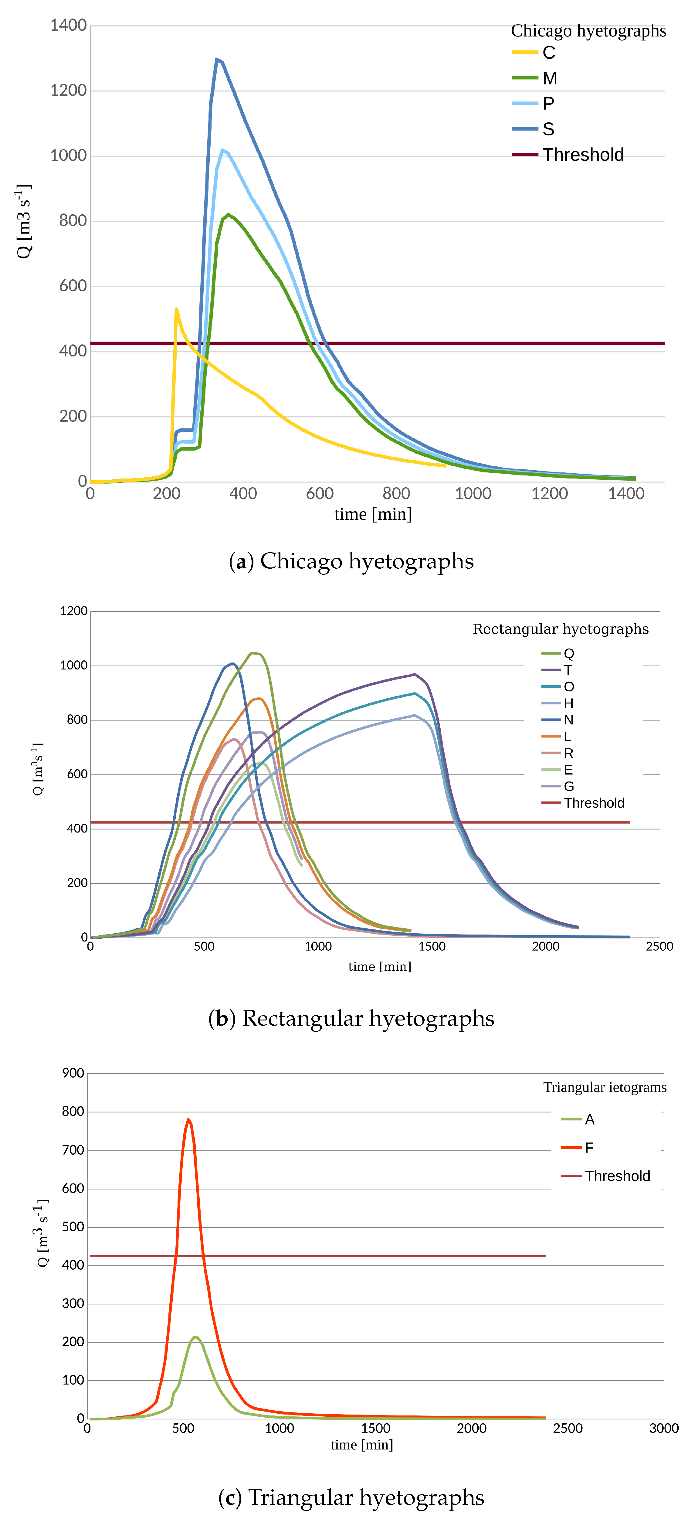
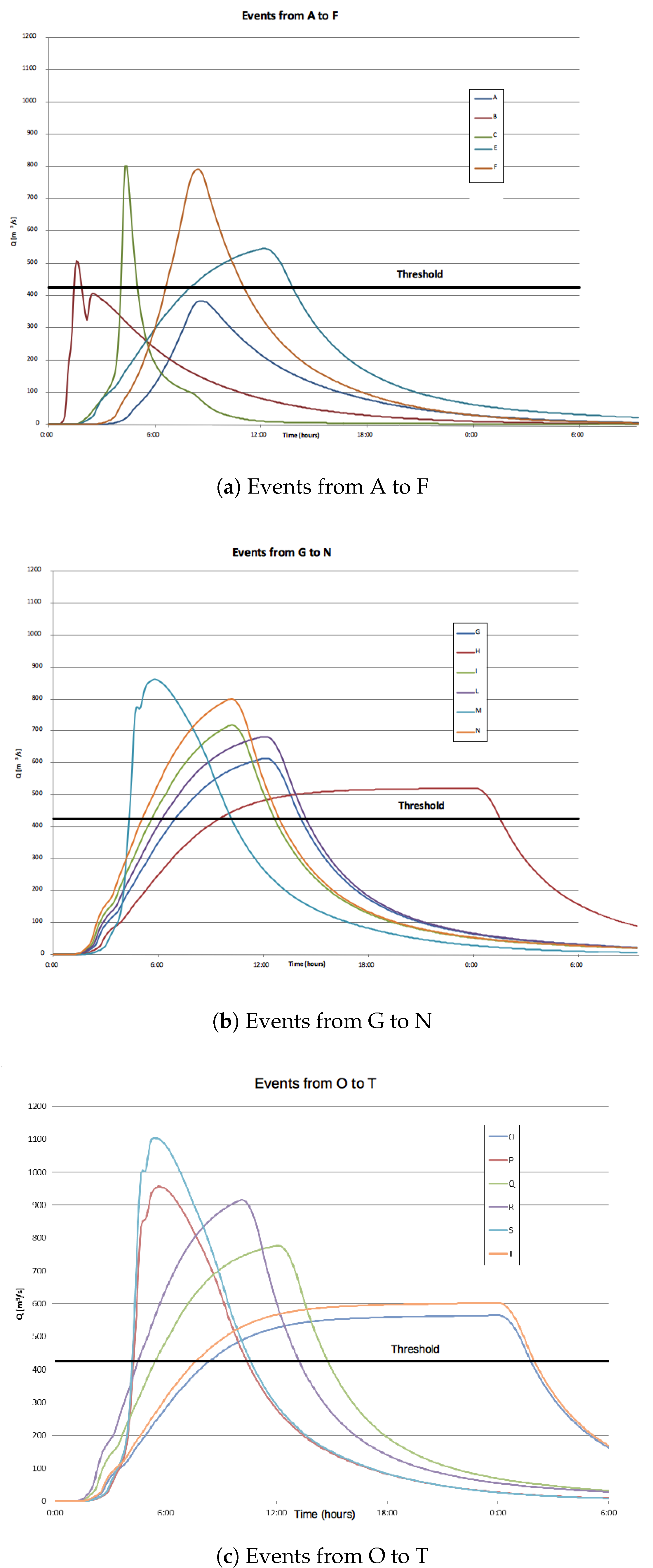
3.1. Comparison of the Hydraulic Parameters and 1D/2D Flood Maps

The seventeen rainfall-runoff events modelled by SWMM, using as many synthetic hydrographs, produced peak flows (Q) in the range 213–1297 m³s⁻¹, with overflow times from 0.5 to 18.3 h. Fifteen of the 17 modelled events determined an overflow limit (Q’) of 425 m³s⁻¹; for these rainfall-runoff events the overflow volume (V_f) varied from 0.13 to 24.2 × 10⁶ m³ (

Table 5. Comparison among hydrographs simulated by SWMM and MIKE FLOOD models in Corace watershed (Calabria, Italy) (n = 17 rainfall-runoff events).

Synthetic	Q [m3s−1]		${\mathit{V}}_{\mathit{f}}$ [Mm3]		T [h]		Q’ [m3s−1]
Hydrograph	SWMM	MIKE	SWMM	MIKE	SWMM	MIKE	SWMM	MIKE
A	214	383	0.00	0.00	0.0	0.0	0	0
B	228	507	0.00	0.09	0.0	0.4	0	58
C	531	802	0.13	0.71	0.5	0.9	74	210
E	643	546	2.54	1.54	4.8	5.8	148	74
F	356	792	1.88	3.05	2.5	4.5	209	190
G	756	614	4.81	3.09	6.0	7.2	223	120
H	818	521	15.40	4.40	16.3	16.0	263	77
I	868	718	5.82	4.42	6.0	7.0	269	175
L	879	682	7.49	4.85	7.3	8.2	287	164
M	820	861	3.80	5.88	4.5	5.8	235	280
N	1007	800	8.61	6.34	6.8	7.8	354	225
O	898	564	20.03	7.00	17.5	17.3	318	112
P	1019	956	6.05	7.34	5.0	6.1	336	335
Q	1046	776	11.70	7.58	8.8	9.3	371	226
R	729	915	3.40	9.23	5.0	8.7	189	294
S	1297	1104	9.51	9.41	5.3	6.4	503	408
T	968	602	24.22	9.42	18.3	18.3	369	143

). The event with the highest runoff volume was produced by the hydrograph T (Chicago, T_r = 500 year, t = 7.6 h, and h = 348.1 mm), while the highest peak flow followed the hydrograph S (Rectangular, T_r = 500 year, t = 24 h, and h = 193.4 mm) (Figure 7 and Figure 8). This means that the largest flood volume was not produced by the event with the highest peak flow.

If the hydraulic variables simulated by SWMM are compared to the corresponding variables produced by MIKE models, differences of 7.1% and 32.7% were found for mean V_f and Q, respectively, while the differences in the mean T and Q’ were 13.6% and 25.5%. The evaluation criteria adopted for model comparison gave low values of r², E, CRM and RMSE. The values of the criteria were below the acceptance limits mentioned above for Q, V_f and Q’, and satisfactory only for T. By contrast, the CRM was fair for both models (

Table 6. Values of the criteria adopted for comparing the hydraulic variables simulated by SWMM and MIKE models in the Corace torrent (Calabria, Southern Italy).

	Hydraulic Variable
	Q		V${}_{\mathit{f}}$		T		Q’
Model	SWMM	MIKE	SWMM	MIKE	SWMM	MIKE	SWMM	MIKE
Mean	769	714	7.38	4.96	6.72	7.63	244	182
Minimum	214	383	0.00	0.00	0.00	0.00	0	0
Maximum	1297	1104	24,22	9.42	18.25	18.28	503	408
Standard Deviation	296	187	7.01	3.19	5.64	5.35	135	107
r2	0.34		0.42		0.97		0.39
RMSE	241		5.87		1.29		121
CRM	0.07		0.33		−0.14		0.25

). The differences in excess volumes and peak flows for the modelled rainfall-runoff events can be also visually noticed from the V-Q plot, which shows how much each event simulated by SWMM is far from the corresponding event predicted by MIKE models (Figure 9).

Comparing the water depths of the flood maps generated by the 17 rainfall-runoff, noticeable differences emerge between 1D and 2D models, for the same simulated event. In terms of mean and maximum flood depths, the highest differences are equal to 0.45 and 2.45 m, respectively (hyetograph A). The extension of the flooded area foreseen by SWMM is larger than that simulated by MIKE models, except in four cases only (hyetographs C, M, P, and S). As an example, Figure 10 shows the comparison between the flooded urban areas predicted by the two models, for the event produced by the hyetograph S.

3.2. 2D Map Selection Using the Similarity Method

The 1D-2D maps cannot be associated using the scatterplot Q-V_f of Figure 9 or the criteria adopted to evaluate the differences among the hydraulic variables predicted by SWMM and MIKE models (Table 5). The similarity method based on the ranking approach is suggested instead to select the 1D map resulting more similar to the 2D map.

Following some authors [58,59], who suggested the use of Spearman’s rank correlation among hydraulic variables, the Spearman index was calculated as

$$\rho =1-\frac{6\sum {d_i}^2}{n(n^2-1)},$$

(9)

where i is the event considered, $X_i$ the rank of peak, $Y_i$ the rank of volume, $d_i$ is the rank of $X_i$ minus rank of $Y_i$, n is the number of events. In the studied watershed, this index was over 0.50 for all the indicators with peak values (over 0.80) for V_f, T, $\frac{IgE}{Io}$, $\frac{IgN}{Io}$ and $\frac{IgE-IgN}{Io}$ (Figure 11). This means that the maps generated by the two models (SWMM and MIKE) for the same hyetograph shows a high similarity in the areal distribution of the flood depths. When the ranks of indicators among the 17 synthetic hyetographs are calculated for both SWMM and MIKE models and reported in the matrix C (

Table 7. Matrix $C$ of the Euclidean distance of the flood maps simulated for 17 rainfall-runoff events using SWMM and MIKE models in the Corace torrent (Calabria, Southern Italy).

Syntetic		SWMM Model
Hyetograph		A	B	C	E	F	G	H	I	L	M	N	O	P	Q	R	S	T
MIKE model	A	9.2	15	32.5	5.6	26.9	15.3	16.1	29	25.1	33.2	38	20.8	40.3	37.5	44.6	45.9	27.3
	B	11	13.2	30.5	5.4	26.4	15.3	15.9	28.8	24.8	32.1	37.8	20.4	39.4	37.3	44.2	45.1	27
	C	34.7	24.8	15.8	30.6	20.9	27.3	30.5	24.2	24.3	17.3	27.3	29.5	22.1	29.3	30.4	26.3	29.9
	E	11.1	13.3	28.2	2.2	21.9	8.9	10.1	23.3	18.6	27.3	32.1	14.1	34.2	31.2	38.3	39.8	20.5
	F	14.7	21	28.5	17.2	11.4	11.4	19.1	12.4	12.8	21.4	20.6	19.7	26	21.4	27.6	30.9	20.7
	G	16.2	17.5	27.1	9.8	18.5	4.4	6	17.8	12.1	22.6	26	7.4	28.8	24.3	31.8	34.1	13.1
	H	26.1	23.7	26.1	20.8	17.4	12.5	14.4	14.8	9.2	17.3	19.7	9.4	21.6	16.6	23.6	25.9	5.5
	I	21.8	25.7	28.8	19.9	13.4	11.1	15.7	7.5	5.2	17.6	15.1	13.4	21	13.7	21.4	25.5	12.2
	L	25.4	21	21.7	19.7	14.5	11.6	14.7	13.8	8.7	13.7	19.3	11.3	19.5	17.2	23.5	24.5	10.3
	M	28.6	23.2	17.9	26.4	7.3	19.4	25.5	11.6	13.6	7.5	14.6	23.3	12.4	16.7	19	17.7	21.4
	N	38.9	38.3	31.8	37.8	18.4	28.5	33.6	14.1	18.7	16.2	5.3	29.8	10.9	7.9	3.6	10.7	24.4
	O	31.4	27.9	25.6	26.4	17.6	17.7	19.9	14.4	10.9	14	16.3	14.8	16.7	13	18.7	20.4	9.3
	P	37.8	34.9	25.9	36.4	15.1	28	33.7	14.5	19.2	11.8	9.1	30.4	7.1	12.5	9.5	8.9	25.9
	Q	37.6	36.2	29.5	35.2	18	25.9	30	13.4	16.1	13.6	7.4	25.8	9.5	6	6.3	10.8	20
	R	19	23.5	28.6	20	10.7	12	18.8	8.2	9.1	19.4	16.1	18	23	16.7	23.2	27.4	17.5
	S	43.9	40.6	30.1	42.2	21.3	33.6	38.9	20.1	24.4	15.7	12.8	35	8.2	15.1	8.5	5.1	29.7
	T	35.6	32.1	27.1	30.9	19.6	22.1	24.4	16	14.2	14	15.3	19.3	14.5	11.7	15.8	17.2	13.4

Note: the blue background in the matrix highlights the main diagonal.

), the most similar 1D-2D maps can be easily selected for possible floods in the urban area downstream of the Corace torrent. The selection was done minimising the vectorial distance between events in the ${\mathbb{R}}^{11}$ space.

In more detail, the following considerations about the method accuracy in choosing the 1D-2D maps corresponding to the same hydrograph can be made (

Table 8. Rank matrix of the Euclidean distance of flood maps simulated by SWMM and MIKE models in the Corace torrent (Calabria, Southern Italy).

Syntetic		SWMM Model
Hyetograph		A	B	C	E	F	G	H	I	L	M	N	O	P	Q	R	S	T
MIKE model	A	1	3	17	3	17	9	7	17	17	17	17	11	17	17	17	17	15
	B	2	1	15	2	16	8	6	16	16	16	16	10	16	16	16	16	14
	C	12	10	1	12	13	14	14	15	14	10	14	14	11	14	13	11	17
	E	3	2	9	1	15	2	2	14	11	15	15	5	15	15	15	15	9
	F	4	5	10	5	3	4	9	4	7	13	12	9	13	12	12	13	10
	G	5	4	8	4	11	1	1	12	6	14	13	1	14	13	14	14	5
	H	9	9	6	9	7	7	3	10	4	9	11	2	10	8	11	10	1
	I	7	11	12	7	4	3	5	1	1	11	6	4	9	6	8	9	4
	L	8	6	3	6	5	5	4	6	2	4	10	3	8	11	10	8	3
	M	10	7	2	10	1	11	12	3	8	1	5	12	5	9	7	6	11
	N	16	16	16	16	10	16	15	7	12	8	1	15	4	2	1	3	12
	O	11	12	4	11	8	10	10	8	5	6	9	6	7	5	6	7	2
	P	15	14	5	15	6	15	16	9	13	2	3	16	1	4	4	2	13
	Q	14	15	13	14	9	13	13	5	10	3	2	13	3	1	2	4	8
	R	6	8	11	8	2	6	8	2	3	12	8	7	12	9	9	12	7
	S	17	17	14	17	14	17	17	13	15	7	4	17	2	7	3	1	16
	T	13	13	7	13	12	12	11	11	9	5	7	8	6	3	5	5	6

Note: the pink background in the matrix highlights the main diagonal.

):

-

for 11 rainfall-runoff events, the minimum distance falls on the main diagonal of the rank matrix, giving a frequency of occurrence of 11/17 (64.7%);

-

this frequency increases to 12 over 17 events (that is, 70.6%), if we accept the possibility of selecting one of the two most similar 1D-2D maps;

-

finally, a frequency of 14/17 = 82.4% is achieved, if the tolerance limit increases to the three most similar 1D-2D maps.

These data show that the proposed method is able to select with an appreciable likelihood (65–82%) the expected 2D-model map, using a simple and quick hydrological-hydraulic prediction tool. Moreover, when the method fails to select the most accurate map (that is the 2D-model map produced by the same hyetograph generating the 1D-model map), the error in estimating the physical variables is still limited. Indeed, considering the percent error on the estimation of the mean flood depth, this error is lower than 4% in the worst case, which corresponds to the simulated event T.

3.3. Proposal for the Method Implementation into an Online Early-Warning Platform for Flood Forecasting

In general, the hazard levels are associated with different thresholds of warning. These thresholds are differentiated for type of hydrological and hydrogeological events (i.e., landslides, inundations, floodings) as well as for an “ongoing” or a “predicted” events. The threshold of the hydrological or hydrogeological events is only based on “ground” observation, typically rainfall, while the dynamics of the ongoing or predicted events is determined on the basis of the weather forecast. More specifically, the determination of the dynamics “ongoing” uses a comparison of rainfall observations at various parts of a given territory and for different event durations, with predetermined specific thresholds for each type of risk, associated with increasing hazard levels.

The use of hydrological and hydraulic mathematical models to calculate the watershed response to a heavy rainfall event allows to better simulate the runoff or flood event generation. The model, therefore, discriminates with a great accuracy the real impact of a meteorological forcing in the territory, according to the current situation of the watershed. Instead, the use of specific thresholds characterised by rainfalls with specific duration and intensity, hypothesises that the ground effects of a given precipitation event is always the same, regardless the season of the year, thus without referring to the influence of recent and past events. This assumption is too simplistic, since it does not take in account the influence of the water content of the soil on the runoff generation capacity. In other words, the same precipitation intensity can lead to a very low discharge in water courses, when occurring after long dry period, but it can originate potentially catastrophic event, if it occurs after a heavy rainfall saturating the soil.

This threshold method can be improved, in order to take into account the water content of the soil and thus the saturation level of the watershed. This evaluation can be made, for example, by evaluating the water content of the soil throughout five days before the modelled event (which is the Antecedent Moisture Condition (AMC) theoretically proposed by the Curve Number method of USDA-SCS). However, this hypothesis, which undoubtedly introduces a certain improvement, is not adequate to take into account the soil saturation and desaturation processes throughout very long periods, due to water losses by evapo-transpiration as well as snowing and melting processes.

All these components are instead considered by the hydrological sub-routines of the SWMM model, which therefore make possible a “continuous” simulation of the hydrological behaviour of a watershed and, as a consequence, its response to precipitation events. The “on-line” use of SWMM (i.e., continuously running in real time) links the real simulation of a rainfall-runoff transformation process to the current hydrological and hydraulic conditions of the watershed. To this aim, a “hot-start” file at the beginning of the simulation is used, which avoids the setup of initial and boundary conditions of the hydrological processes and variables driving the watershed’s hydrological response to a precipitation event. As a matter of fact, the “hot-start” file provides the full hydrologic, hydraulic and water quality conditions of the study area at the end of a model run. The hydrological parameters simulated by the model are used to setup the initial conditions for the subsequent run.

Figure 12 shows a possible implementation of SWMM in an “early warning” system, which runs continuously in a dedicated platform. The first run of the software covers a period of 48 h. The initial time of simulation (indicated as SoS in Figure 12 ) is 24 h before the launching time (Time of Flight “ToF”), which is also the current time. The ending time of the simulated period (End of Simulation, “EoS”) is 24 h after ToF. A half of the model’s input file uses data collected by rain gauges during the 24 h preceding ToF, while the remaining 50% consists of rain forecasts. Of course, the time interval between SoS and EoS is purely representative, because it depends on the Meteorological Service adopted. This hindcasting procedure is needed to refine the model and it runs once. From the second run, the hindcasting period is limited to one hour, and it serves to check whether the model simulations correspond to the real data. The time interval between two consecutive ToFs is one hour. This choice appears to be a reasonable compromise between the need to follow the evolution of the meteorological processes on one side, and the time required to collect and validate the rain gauge data on the other side. The EoS time is updated, after the release of new meteorological forecasts, whose frequency is assumed in 12 h (such as in the case of the Meteorological Center of the Italian Air Force).

The case study of the Corace torrent demonstrated the viability of the proposed method to use a 1D model to forecast floods occurring in urban areas subject to heavy rainfall events.The method selected accurate maps previously prepared using a 1D-2D hydrological-hydraulic model. Thanks to this viability, the method may practically support predictions of real flood events, if integrated in an online early-warning platform, as explained above. This platform generates a real-time flood map assuming as input a weather forecast. The procedure simulates the main hydraulic parameters of the forecasted flood using a 1D model and selects, through the proposed method, a 2D flood map from a catalogue of rainfall-runoff events, generated by a set of synthetic hyetographs, previously simulated by a 1D-2D model.

In more detail, this online early-warning platform operates by the following steps (Figure 13):

-

offline preparation of the event catalogue consisting of flood maps produced by a 1D-2D model applied to a finite number of synthetic hyetographs;

-

construction of the forecasted hyetograph from weather radar predictions;

-

simulation of the corresponding hydrograph and 1D map using the 1D model for the forecasted event in real time;

-

calculation of the n indicators (see Section 2.1.3) used by the proposed method;

-

calculation of $S{r}_j(j=1,n)$ vector in ${\mathbb{N}}^n$;

-

calculation of Euclidean distance among the vector of the forecasted events $S{r}_j$ and all the vectors of maps catalogue $D_r$, which provides the vector $c_l(l=1,m)$∈${\mathbb{R}}^m$;

-

calculation of the vector $e_l$ of the ranks of $c_l$ (distance data in ascending order);

-

selection of the map in the catalogue corresponding to the rank of $e_l$ (thus, having the minimum Euclidean distance from the 1D map) with the cumulative frequency $F_p$.

The selected map is assumed as the flood map for the forecasted event in real time.

The 2D event catalogue of the early warning platform can be integrated by real rainfall-runoff events, detected during the usage. This integration allows a progressive replacement of the synthetic hyetographs with actual hyetographs, hydrographs and the related flood maps.

4. Conclusions

The use of a 1D model to predict flood maps in urban areas may lead to inaccurate predictions. However, a 1D model is often the unique solution to get real-time predictions for small watersheds with a short concentration time, since the use of more accurate 2D models requires run times of the same order of magnitude of the concentration time of the watershed. In order to increase the accuracy of almost real-time flood predictions in urban areas, this study proposed a method to match a flood map simulated by a 1D-2D model, chosen from a set of maps simulated off-line. This method named ranking approach is based on the calculation of the distance in a 11-dimensional space, where variables are a set of hydraulic variables and other geometric indicators (e.g., moments of inertia of the flooded areas) pertaining to the hydraulic response of the watershed to a given rainfall-runoff event. The matching is done with the map with the shortest distance with that generated online by the 1D-model, starting from an actual hyetograph forecasted by a meteorological radar. The method was applied to the Corace torrent (Calabria, Southern Italy), where 17 rainfall-runoff events in response to as many synthetic hyetographs were simulated simultaneously by the 1D SWMM and 1D-2D MIKE models. The 1D and 1D-2D predictions (hydraulic parameters and maps of floods) were compared with each other.

The results of the case study showed not negligible differences between the hydraulic variables (peak flow, flooding time, overflow volume and mean overflow) simulated by the two models. This led to the impossibility to associate the most similar 1D and 2D flood maps through the best matching of indivudual couples of homonym variables. On the contrary, in the case study, the method combined the right 2D map in 65% of the modelled events, and the two or three most similar in 71% and 82% of the cases, respectively. This selection method was also proposed to develop an online early-warning platform for flood prediction, using as input the real-time weather predictions. For this platform, the use of a quick but reliable 1D prediction model seems to be efficient to give flooding alert in case of extreme precipitation events. As a matter of fact, the computation times of the flood maps (of the order of a few minutes) in smallest as well as in biggest watersheds give the authorities the possibility of preparing an effective alert against the flooding risk in urban areas, with the subsequent efficiency in protecting infrastructures and saving human lives. Further method development, preferably using real flood data and a set of representative watersheds with different geomorphological and climatic characteristics, are suggested to evaluate the actual perspectives of the platform implementation. In more detail, a set of real rainfall-runoff events, for which 2D maps are available, could be prepared and the 1D model should be run. The comparison of the 2D maps with those simulated by the 1D model should provide the capability of the proposed method in identifying the most accurate flood map in a sort of pseudo-real time test.

References

1. UNISDR. 2018: Extreme weather events affected 60 million people. In Extreme Weather Events; United Nations Disaster Risk Reduction (UNISDR): New York, NY, USA, 2019. [Google Scholar] [CrossRef]
2. Chen, Y.; Liu, R.; Barrett, D.; Gao, L.; Zhou, M.; Renzullo, L.; Emelyanova, I. A spatial assessment framework for evaluating flood risk under extreme climates. Sci. Total Environ. 2015, 538, 512–523. [Google Scholar] [CrossRef]
3. Sharifan, R.; Roshan, A.; Aflatoni, M.; Jahedi, A.; Zolghadr, M. Uncertainty and Sensitivity Analysis of SWMM Model in Computation of Manhole Water Depth and Subcatchment Peak Flood. Procedia Soc. Behav. Sci. 2010, 2, 7739–7740. [Google Scholar] [CrossRef] [Green Version]
4. Wang, K.; Altunkaynak, A. Comparative Case Study of Rainfall-Runoff Modeling between SWMM and Fuzzy Logic Approach. J. Hydrol. Eng. 2012, 17, 283–291. [Google Scholar] [CrossRef]
5. Kreibich, H.; Van Den Bergh, J.; Bouwer, L.; Bubeck, P.; Ciavola, P.; Green, C.; Hallegatte, S.; Logar, I.; Meyer, V.; Schwarze, R.; et al. Costing natural hazards. Nat. Clim. Chang. 2014, 4, 303–306. [Google Scholar] [CrossRef]
6. Mignot, E.; Li, X.; Dewals, B. Experimental modelling of urban flooding: A review. J. Hydrol. 2019, 568, 334–342. [Google Scholar] [CrossRef] [Green Version]
7. Choi, K.; Ball, J. Parameter estimation for urban runoff modelling. Urban Water 2002, 4, 31–41. [Google Scholar] [CrossRef]
8. Du, J.; Qian, L.; Rui, H.; Zuo, T.; Zheng, D.; Xu, Y.; Xu, C.Y. Assessing the effects of urbanization on annual runoff and flood events using an integrated hydrological modeling system for Qinhuai River basin, China. J. Hydrol. 2012, 464, 127–139. [Google Scholar] [CrossRef]
9. Krebs, G.; Kokkonen, T.; Valtanen, M.; Koivusalo, H.; Setälä, H. A high resolution application of a stormwater management model (SWMM) using genetic parameter optimization. Urban Water J. 2013, 10, 394–410. [Google Scholar] [CrossRef]
10. Sahoo, G.; Ray, C.; De Carlo, E. Calibration and validation of a physically distributed hydrological model, MIKE SHE, to predict streamflow at high frequency in a flashy mountainous Hawaii stream. J. Hydrol. 2006, 327, 94–109. [Google Scholar] [CrossRef]
11. Loi, N.K.; Liem, N.D.; Tu, L.H.; Hong, N.T.; Truong, C.D.; Tram, V.N.Q.; Nhat, T.T.; Anh, T.N.; Jeong, J. Automated procedure of real-time flood forecasting in Vu Gia—Thu Bon river basin, Vietnam by integrating SWAT and HEC-RAS models. J. Water Clim. Chang. 2018, 10, 535–545. [Google Scholar] [CrossRef]
12. Goodall, J.; Morsy, M.; Sadler, J. Real-Time Flood Prediction Using Data-Driven and Hydrodynamic Modeling Tools. Model. Manag. Extrem. Precip. 2017, 10, 535–545. [Google Scholar]
13. Teng, J.; Jakeman, A.; Vaze, J.; Croke, B.; Dutta, D.; Kim, S. Flood inundation modelling: A review of methods, recent advances and uncertainty analysis. Environ. Model. Softw. 2017, 90, 201–216. [Google Scholar] [CrossRef]
14. Follum, M.; Tavakoly, A.; Niemann, J.; Snow, A. AutoRAPID: A Model for Prompt Streamflow Estimation and Flood Inundation Mapping over Regional to Continental Extents. JAWRA J. Am. Water Resour. Assoc. 2016, 53. [Google Scholar] [CrossRef]
15. Zheng, X.; Tarboton, D.G.; Maidment, D.R.; Liu, Y.Y.; Passalacqua, P. River Channel Geometry and Rating Curve Estimation Using Height above the Nearest Drainage. JAWRA J. Am. Water Resour. Assoc. 2018, 54, 785–806. [Google Scholar] [CrossRef]
16. Wang, X.; Kinsland, G.; Poudel, D.; Fenech, A. Urban flood prediction under heavy precipitation. J. Hydrol. 2019, 577, 123984. [Google Scholar] [CrossRef]
17. Dottori, F.; Di Baldassarre, G.; Todini, E. Detailed data is welcome, but with a pinch of salt: Accuracy, precision, and uncertainty in flood inundation modeling. Water Resour. Res. 2013, 49, 6079–6085. [Google Scholar] [CrossRef]
18. Paquier, A.; Mignot, E.; Bazin, P. From hydraulic modelling to urban flood risk. Procedia Eng. 2015, 115, 37–44. [Google Scholar] [CrossRef]
19. Falconer, R.; Xia, J.; Liang, D.; Kvoka, D. Flood modelling and hazard assessment for extreme events in riverine basins. In Proceedings of the 37th IAHR World Congress 2017: Managing Water for Sustainable Development: Learning from the Past for the Future, Kuala Lumpur, Malaysia, 13–18 August 2017; Ghani, A., Ed.; International Assn for Hydro-Environment Engineering and Research (IAHR): Beijing, China, 2017. [Google Scholar]
20. Rong, Y.; Zhang, T.; Zheng, Y.; Hu, C.; Peng, L.; Feng, P. Three-dimensional urban flood inundation simulation based on digital aerial photogrammetry. J. Hydrol. 2019, 584, 124308. [Google Scholar] [CrossRef]
21. Patro, S.; Chatterjee, C.; Mohanty, S.; Singh, R.; Raghuwanshi, N. Flood inundation modeling using MIKE FLOOD and remote sensing data. J. Indian Soc. Remote Sens. 2009, 37, 107–118. [Google Scholar] [CrossRef]
22. Aricò, C.; Filianoti, P.; Sinagra, M.; Tucciarelli, T. The FLO Diffusive 1D-2D Model for Simulation of River Flooding. Water 2016, 8, 200. [Google Scholar] [CrossRef] [Green Version]
23. Phillips, B.; Yu, S.; Thompson, G.; Silva, N. 1D and 2D Modelling of Urban Drainage Systems using XP-SWMM and TUFLOW. In Proceedings of the 10th International Conference on Urban Drainage, Copenhagen, Denmark, 21–26 August 2005. [Google Scholar]
24. Barco, J.; Wong, K.; Stenstrom, M. Automatic calibration of the U.S. EPA SWMM model for a large urban catchment. J. Hydraul. Eng. 2008, 134, 466–474. [Google Scholar] [CrossRef]
25. Henonin, J.; Russo, B.; Mark, O.; Gourbesville, P. Real-time urban flood forecasting and modelling—A state of the art. J. Hydroinform. 2013, 15, 717–736. [Google Scholar] [CrossRef]
26. Jamali, B.; Löwe, R.; Bach, P.M.; Urich, C.; Arnbjerg-Nielsen, K.; Deletic, A. A rapid urban flood inundation and damage assessment model. J. Hydrol. 2018, 564, 1085–1098. [Google Scholar] [CrossRef]
27. Lee, S.; Lee, S.; Lee, M.J.; Jung, H.S. Spatial Assessment of Urban Flood Susceptibility Using Data Mining and Geographic Information System (GIS) Tools. Sustainability 2018, 10, 648. [Google Scholar] [CrossRef] [Green Version]
28. Zema, D.; Labate, A.; Martino, D.; Zimbone, S. Comparing Different Infiltration Methods of the HEC-HMS Model: The Case Study of the Mésima Torrent (Southern Italy). Land Degrad. Dev. 2017, 28, 294–308. [Google Scholar] [CrossRef]
29. Bisht, D.; Chatterjee, C.; Kalakoti, S.; Upadhyay, P.; Sahoo, M.; Panda, A. Modeling urban floods and drainage using SWMM and MIKE URBAN: A case study. Nat. Hazards 2016, 84, 749–776. [Google Scholar] [CrossRef]
30. Papaioannou, G.; Loukas, A.; Vasiliades, L.; Aronica, G. Flood inundation mapping sensitivity to riverine spatial resolution and modelling approach. Nat. Hazards 2016, 83, 117–132. [Google Scholar] [CrossRef]
31. Kourtis, I.; Bellos, V.; Tsihrintzis, V. Comparison of 1D-1D and 1D-2D urban flood models. In Proceedings of the 15th International Conference on Environmental Science and Technology, Rhodes, Greece, 31 August–2 September 2017. [Google Scholar]
32. Leandro, J.; Chen, A.S.; Djordjević, S.; Savic, D. Comparison of 1D/1D and 1D/2D Coupled (Sewer/Surface) Hydraulic Models for Urban Flood Simulation. J. Hydraul. Eng. 2009, 135, 495–504. [Google Scholar] [CrossRef]
33. Leandro, J.; Djordjević, S.; Chen, A.; Savić, D.; Stanić, M. Calibration of a 1D/1D urban flood model using 1D/2D model results in the absence of field data. Water Sci. Technol. 2011, 64, 1016–1024. [Google Scholar] [CrossRef] [Green Version]
34. Fortugno, D.; Boix-Fayos, C.; Bombino, G.; Denisi, P.; Quiñonero Rubio, J.; Tamburino, V.; Zema, D. Adjustments in channel morphology due to land-use changes and check dam installation in mountain torrents of Calabria (southern Italy). Earth Surf. Process. Landf. 2017, 42, 2469–2483. [Google Scholar] [CrossRef]
35. Zema, D.; Lucas-Borja, M.; Carrá, B.; Denisi, P.; Rodrigues, V.; Ranzini, M.; Arcova, F.; de Cicco, V.; Zimbone, S. Simulating the hydrological response of a small tropical forest watershed (Mata Atlantica, Brazil) by the AnnAGNPS model. Sci. Total Environ. 2018, 636, 737–750. [Google Scholar] [CrossRef] [PubMed] [Green Version]
36. Huber, W.; Dickinson, R.; Rossman, L. EPA Storm Water Management Model, SWMM5. In Watershed Models; US Environmental Protection Agency (EPA): Washington, DC, USA, 2010. [Google Scholar] [CrossRef]
37. Willmott, C.; Cort, J. Some comments on the evaluation of model performance. Bull. Am. Meteorol. Soc. 1982, 100, 1309–1313. [Google Scholar] [CrossRef] [Green Version]
38. Legates, D.; McCabe, G. Evaluating the use of “goodness-of-fit” measures in hydrologic and hydroclimatic model validation. Water Resour. Res. 1999, 35, 233–241. [Google Scholar] [CrossRef]
39. Loague, K.; Green, R. Statistical and graphical methods for evaluating solute transport models: Overview and application. J. Contam. Hydrol. 1991, 7, 51–73. [Google Scholar] [CrossRef]
40. Zema, D.; Bingner, R.L.; Denisi, P.; Govers, G.; Licciardello, F.; Zimbone, S. Evaluation of runoff, peak flowand sediment yield for events simulated by the annagnps model in a belgian agricultural watershed. Land Degrad. Dev. 2012, 23, 205–215. [Google Scholar] [CrossRef]
41. Krause, P.; Boyle, D.; Báse, F. Comparison of different efficiency criteria for hydrological model assessment. Adv. Geosci. 2005, 5, 89–97. [Google Scholar] [CrossRef] [Green Version]
42. Moriasi, D.; Arnold, J.; Van Liew, M.; Bingner, R.; Harmel, R.; Veith, T. Model evaluation guidelines for systematic quantification of accuracy in watershed simulations. Trans. ASABE 2007, 50, 885–900. [Google Scholar] [CrossRef]
43. Van Liew, M.W.; Garbrecht, J. Hydrologic simulation of little wrew using SWAT. JAWRA J. Am. Water Resour. Assoc. 2003, 39, 413–426. [Google Scholar] [CrossRef]
44. Santhi, C.; Arnold, J.; Williams, J.; Dugas, W.; Srinivasan, R.; Hauck, L. Validation of the Swat Model on a Large Rwer Basin With Point and Nonpoint Sources. JAWRA J. Am. Water Resour. Assoc. 2001, 37, 1169–1188. [Google Scholar] [CrossRef]
45. Vieira, D.; Serpa, D.; Nunes, J.; Prats, S.; Neves, R.; Keizer, J. Predicting the effectiveness of different mulching techniques in reducing post-fire runoff and erosion at plot scale with the RUSLE, MMF and PESERA models. Environ. Res. 2018, 165, 365–378. [Google Scholar] [CrossRef]
46. Nash, J.; Sutcliffe, J. River flow forecasting through conceptual models. Part I: A discussion of principles. J. Hydrol. 1970, 10, 282–290. [Google Scholar] [CrossRef]
47. Fernández, C.; Vega, J.; Vieira, D. Assessing soil erosion after fire and rehabilitation treatments in NW Spain: Performance of RUSLE and revised Morgan–Morgan–Finney models. Land Degrad. Dev. 2010, 21, 58–67. [Google Scholar] [CrossRef] [Green Version]
48. Singh, J.; Knapp, H.; Arnold, J.; Demissie, M. Hydrological modeling of the Iroquois river watershed using HSPF and SWAT. JAWRA J. Am. Water Resour. Assoc. 2005, 41, 343–360. [Google Scholar] [CrossRef]
49. Gupta, H.; Sorooshian, S.; Yapo, P. Status of automatic calibration for hydrologic models: Comparison with multilevel expert calibration. J. Hydrol. Eng. 1999, 4, 135–143. [Google Scholar] [CrossRef]
50. Cai, C.; Wang, J.; Li, Z. Assessment and modelling of uncertainty in precipitation forecasts from TIGGE using fuzzy probability and Bayesian theory. J. Hydrol. 2019, 577, 123995. [Google Scholar] [CrossRef]
51. Chen, L.; Singh, V.P.; Lu, W.; Zhang, J.; Zhou, J.; Guo, S. Streamflow forecast uncertainty evolution and its effect on real-time reservoir operation. J. Hydrol. 2016, 540, 712–726. [Google Scholar] [CrossRef]
52. Chow, V.; Maidment, D.; Mays, L. Applied Hydrology; MacGraw-Hill: New York, USA, 1988. [Google Scholar]
53. Kirpich, Z. Time of concentration of small watersheds. J. Civ. Eng. (ASCE) 1940, 10, 362. [Google Scholar]
54. European Environment Agency. CORINE Land Cover; European Environment Agency (EEA): Copenhagen, Denmark, 2006. Available online: https://land.copernicus.eu/pan-european/corine-land-cover/clc-2006 (accessed on 19 November 2019).
55. Huber, W.C.; Dickinson, R. Storm Water Management Model, Version 4: Users Manual; Environmental Research Laboratory, EPA: Washington, DC, USA, 1988.
56. Rossman, L. Storm Water Management Model User’s Manual Version 5.0; National Risk Management Research Laboratory: Washington, DC, USA, 2009. [Google Scholar]
57. Gironás, J.; Roesner, L.; Rossman, L.; Davis, J. A new applications manual for the Storm Water Management Model (SWMM). Environ. Model. Softw. 2010, 25, 813–814. [Google Scholar] [CrossRef]
58. Gaál, L.; Szolgay, J.; Kohnová, S.; Hlavˇcová, K.; Parajka, J.; Viglione, A.; Merz, R.; Blöschl, G. Dependence between flood peaks and volumes: A case study on climate and hydrological controls. Hydrol. Sci. J. 2014, 60, 968–984. [Google Scholar] [CrossRef] [Green Version]
59. Gaál, L.; Szolgay, J.; Kohnová, S.; Hlavčová, K.; Parajka, J.; Viglione, A.; Merz, R.; Blöschl, G. Relation entre pics et volumes de crues: Étude des déterminants climatiques et hydrologiques. Hydrol. Sci. J. 2015, 60, 968–984. [Google Scholar] [CrossRef] [Green Version]
Figure 1. Scheme of a flood hydrograph with the main hydraulic parameters.
Water 12 01525 g001
Figure 2. Flow chart of the procedure adopted to compare the hydraulic parameters of extreme flood events simulated by 1D and 2D models.
Water 12 01525 g002
Figure 3. North and east coordinates of each pixel data and depth value ( x i , y i , h i ) of a flood map processed by the proposed method.
Water 12 01525 g003
Figure 4. Location, drainage area and hydrographic network of Corace watershed (Calabria, Southern Italy).
Water 12 01525 g004
Figure 5. Discretisation of the Corace watershed (Calabria, Southern Italy) in hydrologically homogenous units using the SWMM model ((a) entire watershed; (b) urban area with the delineated sub-watersheds.
Water 12 01525 g005
Figure 6. Discretisation of the Corace watershed (Calabria, Southern Italy) in hydrologically homogenous units using the MIKE models ((a) entire watershed; (b) urban area with the delineated sub-watersheds-in red lines-and the sub-surface drainage network-in yellow lines).
Water 12 01525 g006
Figure 7. Hydrographs simulated by SWMM model in Corace watershed (Calabria, Italy) for n = 17 rainfall-runoff events, using as input (a) Chicago, (b) rectangular and (c) triangular hyetographs.
Water 12 01525 g007
Figure 8. Hydrographs simulated by MIKE model in Corace watershed (Calabria, Italy) for n = 17 rainfall-runoff events.
Water 12 01525 g008
Figure 9. Plot of the 17 rainfall-runoff events simulated by SWMM and MIKE models in the Corace torrent (Calabria, Southern Italy).
Water 12 01525 g009
Figure 10. Map of the flooded area predicted by the SWMM (a) and MIKE (b) models using the synthetic hyetograph “S” in the Corace torrent (Calabria, Southern Italy).
Water 12 01525 g010
Figure 11. Spearman’s index calculated for the 11 indicators of 1D-2D map similarity for the 17 rainfall-runoff events simulated by SWMM and MIKE models in the Corace torrent (Calabria, Southern Italy).
Water 12 01525 g011
Figure 12. Sequences of run of SWMM software, in an “on-line” early warning system.
Water 12 01525 g012
Figure 13. Flow chart of an online early-warning platform for flood forecasting using the proposed method.
Water 12 01525 g013