Teleconnections between Monthly Rainfall Variability and Large-Scale Climate Indices in Southwestern Colombia

 ,
,  ,
,  , and
, and
Abstract
1. Introduction
2. Data and Methods
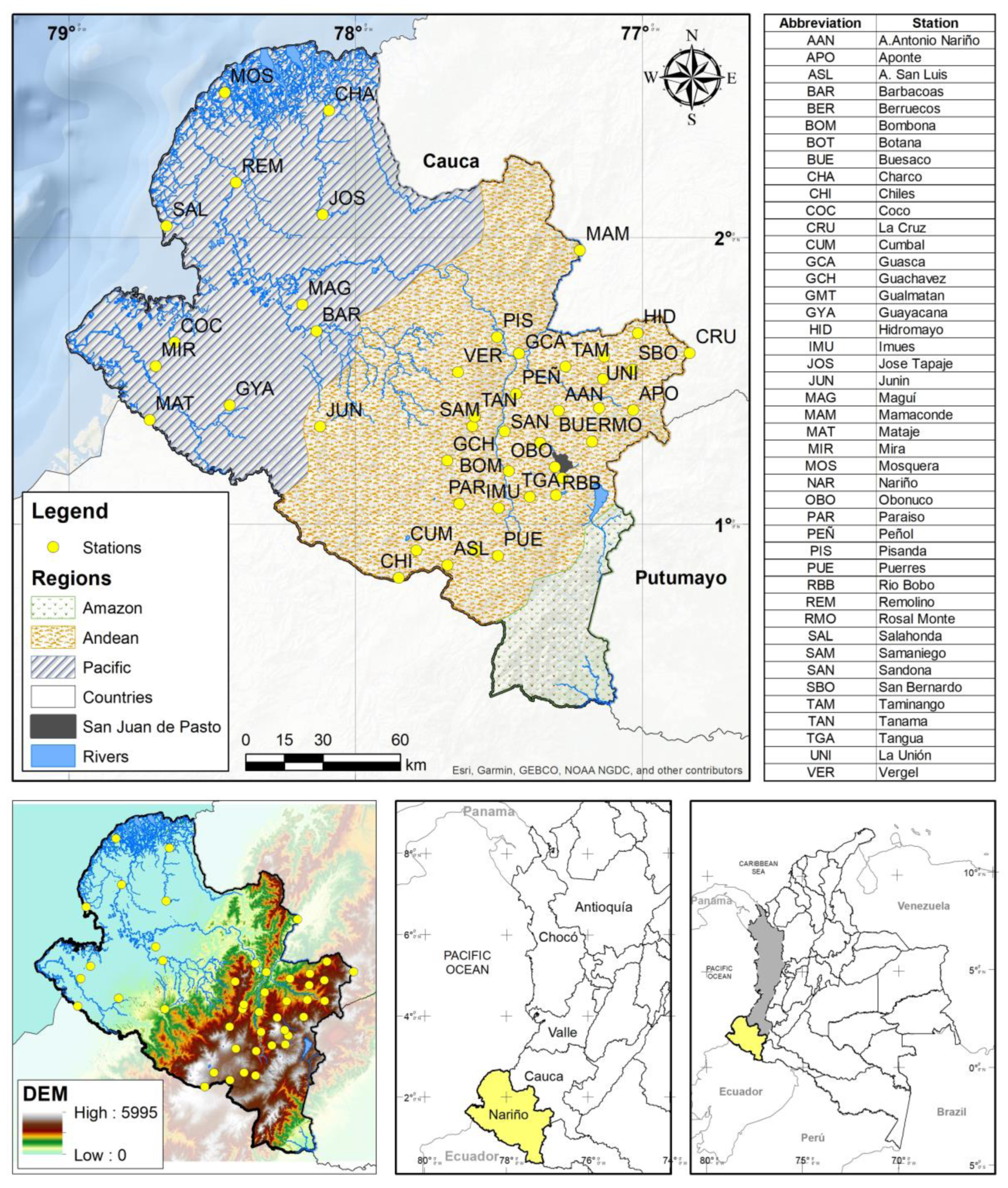
2.1. Study Area
2.2. Rainfall Dataset
2.3. Climate-Oceanographic Indices
2.4. Regionalization of Monthly Rainfall
2.5. Nonlinear Principal Component Analysis
2.6. Teleconnections
3. Results and Discussion
3.1. Missing Data Estimation
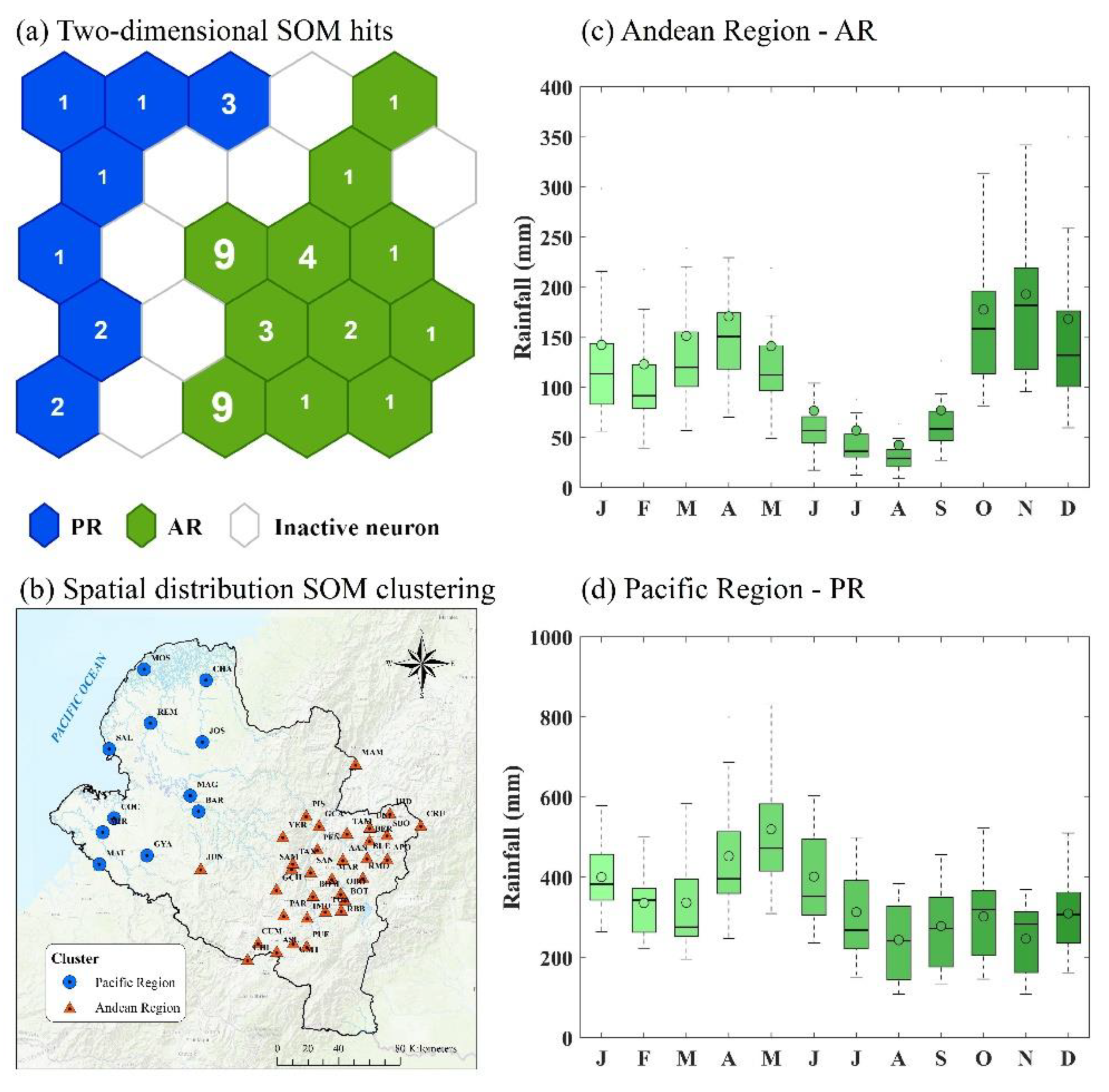
3.2. Regionalization of Monthly Rainfall
3.3. Nonlinear Principal Component Analysis
3.4. Teleconnections
4. Conclusions
- From the NLPCA, we found two main modes of variability in AR and one in PR that explained around 75% and 48% of the variance of the original datasets, respectively. The positive (negative) periods of NLPC1-AR and NLPC2-AR coincided with the LN (EN) events. In contrast, those positive (negative) periods of NLPC1-PR coincided with EN (LN) events, i.e., the variability of monthly rainfall in the Andean region is contrary to the variability of monthly rainfall in the Nariño coastal region. The variability of monthly rainfall in AR is similar to the variability of rainfall in most of the Colombian territory, and the variability of monthly rainfall in PR is similar to the variability of rainfall that is registered in the coastal region of the border country, Ecuador.
- The Pearson’s Correlation between NLPCs of AR and PR and eight climate-oceanographic indices showed that the rainfall in AR has a direct (inverse) relationship with the SOI (ONI, MEI, Niño1 + 2, Niño3, Niño3.4, Niño4, and PDO) indices. Furthermore, the magnitude of the correlations was strongest with Niño3.4 and Niño4, and this influence remained for 10 and eight months, respectively. In this regard, the rainfall in PR showed positive synchronous correlations, but non-statistical significance with Niño1 + 2 and Niño3 indices, and an inverse relationship with Niño3.4 and Niño4 in 8, 9, and 10-lags. Overall, indices that were linked to the ENSO phenomenon showed strong teleconnections with the rainfall in AR, and weak ones in PR. The established results allow us to infer that the variability of rainfall in Southwestern Colombia influences the ENSO’s inter-annual phenomenon its influence is stronger in east Nariño than on the west. These results are especially important for subsequent prediction analyses, given that the climate-oceanographic-indices with high synchronous and lagging correlation could become potential predictors of monthly rainfall in these sub-regions of Southwestern Colombia.
- Wavelet Coherence analysis confirmed the relationships between ENSO indices and rainfall of AR and PR, which showed that the variability of the rain in AR is strongly influenced by the ENSO indices, mainly by the SST in the regions Niño3.4 and Niño4 on the 3–7-year inter-annual scale. Furthermore, this analysis ratified the weak influence of the ENSO phenomenon on PR rainfall. However, we noticed that, in the 1.5–3-year inter-annual scale, there is an influence of the SST in the region Niño3. Overall, the rain in AR is associated to the SST in the east TPO (Niño3.4, Niño4, ONI, and MEI), where the warm (cold) phase of ENSO led to dry (wet) conditions for approximately 5–11 months. Meanwhile, the rainfall of PR is associated to the SST in the center of TPO (Niño3), where the warm (cold) phase of ENSO led to wet (dry) conditions for approximately 1–5 months.
- The main findings of this research study are an understanding of the monthly variability rainfall in AR and PR, in Southwestern Colombia concerning the teleconnections with eight climate indices (when considering the multi-scale relations). This study allowed for us to establish for the first time the contrary relationships between ENSO indices and monthly rainfall in the sub-regions studied, where the EN events lead to a decrease (increase) in the monthly rainfall on AR (PR), while the opposite occurred in the LN events. The ENSO influence on the rainfall of the AR is highly correlated, and it has similar behavior to the impact of ENSO over most of the Colombian territory. In contrast, the findings revealed that the ENSO influence on PR is weak, showing similarities with the ENSO influence over the rainfall in the neighboring country of Ecuador. These results show that future studies need to explore the ocean-atmospheric and regional circulation processes that explain the marked difference in the relationships between ENSO and the region’s rainfall.
Author Contributions
Funding
Conflicts of Interest
References
- Coulibaly, P. Spatial and temporal variability of Canadian seasonal precipitation (1900–2000). Adv. Water Resour. 2006, 29, 1846–1865. [Google Scholar] [CrossRef]
- Min, S.-K.; Zhang, X.; Zwiers, F.W.; Hegerl, G.C. Human contribution to more-intense precipitation extremes. Nature 2011, 470, 378–381. [Google Scholar] [CrossRef]
- Xiao, M.; Zhang, Q.; Singh, V.P. Spatiotemporal variations of extreme precipitation regimes during 1961–2010 and possible teleconnections with climate indices across China. Int. J. Climatol. 2017, 37, 468–479. [Google Scholar] [CrossRef]
- Schulte, J.A.; Najjar, R.G.; Li, M. The influence of climate modes on streamflow in the Mid-Atlantic region of the United States. J. Hydrol. Reg. Stud. 2016, 5, 80–99. [Google Scholar] [CrossRef]
- Kim, T.; Shin, J.-Y.; Kim, S.; Heo, J.-H. Identification of relationships between climate indices and long-term precipitation in South Korea using ensemble empirical mode decomposition. J. Hydrol. 2018, 557, 726–739. [Google Scholar] [CrossRef]
- Cai, W.; McPhaden, M.J.; Grimm, A.M.; Rodrigues, R.R.; Taschetto, A.S.; Garreaud, R.D.; Dewitte, B.; Poveda, G.; Ham, Y.-G.; Santoso, A. Climate impacts of the El Niño–Southern Oscillation on South America. Nat. Rev. Earth Environ. 2020, 1, 215–231. [Google Scholar] [CrossRef]
- Montealegre, E.J.; Pabón, J.D. La variabilidad climática interanual asociada al ciclo El Niño-La Niña-Oscilación del Sur y su efecto en el patrón pluviométrico de Colombia. Meteorol. Colomb. 2000, 2, 7–21. [Google Scholar]
- Poveda, G.; Jaramillo, A.; Gil, M.M.; Quiceno, N.; Mantilla, R.I. Seasonally in ENSO-related precipitation, river discharges, soil moisture, and vegetation index in Colombia. Water Resour. Res. 2001, 37, 2169–2178. [Google Scholar] [CrossRef]
- Ávila; Javier, D.Á.; Carvajal Escobar, Y.; Gutiérrez Serna, S.E. Análisis de la influencia de El Niño y La Niña en la oferta hídrica mensual de la cuenca del río Cali. Tecnura 2013, 18, 120–133. [Google Scholar]
- Poveda, G.; Vélez, J.; Mesa, O.; Hoyos, C.; Mejía, J.F.; Barco, O.J.; Correa, P.L. Influencia de fenómenos macroclimáticos sobre el ciclo anual de la hidrología colombiana: Cuantificación lineal, no lineal y percentiles probabilísticos. Meteorol. Colomb. 2002, 6, 121–130. [Google Scholar]
- Canchala, T.; Loaiza Cerón, W.; Francés, F.; Carvajal-Escobar, Y.; Andreoli, R.V.; Kayano, M.T.; Alfonso-Morales, W.; Caicedo-Bravo, E.; Ferreira de Souza, R.A. Streamflow Variability in Colombian Pacific Basins and Their Teleconnections with Climate Indices. Water 2020, 12, 526. [Google Scholar] [CrossRef]
- Loaiza, W.; Carvajal-Escobar, Y.; Andreoli, R.V.; Kayano, M.T.; Gonzáles, N. Spatio-temporal variability of the droughts in Cali, Colombia and their relationships with the El Niño-Southern Oscillation (ENSO) between 1971 and 2011. Atmósfera 2020, 33, 51–69. [Google Scholar] [CrossRef]
- Jaramillo, L.; Poveda, G.; Mejía, J.F. Mesoscale convective systems and other precipitation features over the tropical Americas and surrounding seas as seen by TRMM. Int. J. Climatol. 2017, 37, 380–397. [Google Scholar] [CrossRef]
- Yepes, J.; Poveda, G.; Mejía, J.F.; Moreno, L.; Rueda, C. CHOCO-JEX: A research experiment focused on the CHOCO low-level jet over the far Eastern Pacific and Western Colombia. Bull. Am. Meteorol. Soc. 2019, 100, 779–796. [Google Scholar] [CrossRef]
- Espinoza, J.C.; Garreaud, R.; Poveda, G.; Arias, P.A.; Molina-Carpio, J.; Masiokas, M.; Viale, M.; Scaff, L. Hydroclimate of the Andes Part I: Main climatic features. Front. Earth Sci. 2020, 8, 64. [Google Scholar] [CrossRef]
- Poveda, G.; Jaramillo, L.; Vallejo, L.F. Seasonal precipitation patterns along pathways of South American low-level jets and aerial rivers. Water Resour. Res. 2014, 50, 98–118. [Google Scholar] [CrossRef]
- Poveda, G.; Mesa, O. La corriente de chorro superficial del Oeste (“del Chocó”) y otras dos corrientes de chorro en Colombia: Climatología y variabilidad durante las fases del ENSO”. Rev. Acad. Colomb. Cienc. 1999, 23, 517–528. [Google Scholar]
- Vuille, M.; Bradley, R.S.; Keimig, F. Interannual climate variability in the Central Andes and its relation to tropical Pacific and Atlantic forcing. J. Geophys. Res. Atmos. 2000, 105, 12447–12460. [Google Scholar] [CrossRef]
- Villacis, M.; Taupin, J.D. Variabilité climatique dans la sierra équatorienne en relation avec le phénomène ENSO. In Proceedings of the International Conference on Hydrology of the Mediterranean and Semi-Arid Regions, Montpellier, France, 1–4 April 2003; p. 202. [Google Scholar]
- Hurtado, A. Estimación de los Campos Mensuales Históricos de Precipitación en el Territorio Colombiano. Master’s Thesis, Universidad Nacional de Colombia, Medellin, Colombia, December 2009. [Google Scholar]
- Poveda, G.; Álvarez, D.M.; Rueda, Ó.A. Hydro-climatic variability over the Andes of Colombia associated with ENSO: A review of climatic processes and their impact on one of the Earth’s most important biodiversity hotspots. Clim. Dyn. 2011, 36, 2233–2249. [Google Scholar] [CrossRef]
- Tootle, G.A.; Piechota, T.C.; Gutiérrez, F. The relationships between Pacific and Atlantic Ocean sea surface temperatures and Colombian streamflow variability. J. Hydrol. 2008, 349, 268–276. [Google Scholar] [CrossRef]
- Rojo, J.D.; Carvajal, L.F. Predicción no lineal de caudales utilizando variables macroclimáticas y análisis espectral singular. Tecnol. Cienc. Agua 2010, 1, 59–73. [Google Scholar]
- Rodríguez-Rubio, E. A multivariate climate index for the western coast of Colombia. Adv. Geosci. 2013, 33, 21–26. [Google Scholar] [CrossRef]
- Córdoba-Machado, S.; Palomino-Lemus, R.; Gámiz-Fortis, S.R.; Castro-Díez, Y.; Esteban-Parra, M.J. Influence of tropical Pacific SST on seasonal precipitation in Colombia: Prediction using El Niño and El Niño Modoki. Clim. Dyn. 2015, 44, 1293–1310. [Google Scholar] [CrossRef]
- Cuadrado, P.B.; Blanco, R.J. Teleconexiones y eventos extremos de sequía en áreas protegidas del norte de Colombia. Rev. Climatol. 2015, 15, 27–38. [Google Scholar]
- Restrepo, J.C.; Higgins, A.; Escobar, J.; Ospino, S.; Hoyos, N. Contribution of low-frequency climatic–oceanic oscillations to streamflow variability in small, coastal rivers of the Sierra Nevada de Santa Marta (Colombia). Hydrol. Earth Syst. Sci. 2019, 23, 2379–2400. [Google Scholar] [CrossRef]
- Canchala, T.; Carvajal-Escobar, Y.; Alfonso-Morales, W.; Loaiza, W.; Caicedo, E. Estimation of missing data of monthly rainfall in southwestern Colombia using artificial neural networks. Data Br. 2019. [Google Scholar] [CrossRef]
- Scholz, M.; Kaplan, F.; Guy, C.L.; Kopka, J.; Selbig, J. Non-linear PCA: A missing data approach. Bioinformatics 2005, 21, 3887–3895. [Google Scholar] [CrossRef]
- Carvajal, Y.; Grisales, C.; Mateus, J. Correlación de variables macroclimáticas del Océano Pacífico con los caudales en los ríos interandinos del Valle del Cauca (Colombia). Rev. Peru. Biol. 1999, 6, 9–17. [Google Scholar] [CrossRef][Green Version]
- Poveda, G. La hidroclimatología de Colombia: Una síntesis desde la escala inter-decadal hasta la escala diurna. Rev. Acad. Colomb. Cienc. 2004, 28, 201–222. [Google Scholar]
- Puertas, O.; Carvajal, Y.E. Incidence of El Niño southern oscillation in the precipitation and the temperature of the air in Colombia, using Climate Explorer. Ing. Desarro. 2008, 23, 104–118. [Google Scholar]
- Wolter, K.; Timlin, M.S. El Niño/Southern Oscillation behaviour since 1871 as diagnosed in an extended multivariate ENSO index (MEI. ext). Int. J. Climatol. 2011, 31, 1074–1087. [Google Scholar] [CrossRef]
- L’Heureux, M.L.; Collins, D.C.; Hu, Z.-Z. Linear trends in sea surface temperature of the tropical Pacific Ocean and implications for the El Niño-Southern Oscillation. Clim. Dyn. 2013, 40, 1223–1236. [Google Scholar] [CrossRef]
- Mantua, N.J.; Hare, S.R.; Zhang, Y.; Wallace, J.M.; Francis, R.C. A Pacific interdecadal climate oscillation with impacts on salmon production. Bull. Am. Meteorol. Soc. 1997, 78, 1069–1080. [Google Scholar] [CrossRef]
- Hsieh, W.W.; Tang, B. Applying neural network models to prediction and data analysis in meteorology and oceanography. Bull. Am. Meteorol. Soc. 1998, 79, 1855–1870. [Google Scholar] [CrossRef]
- Kohonen, T.; Hynninen, J.; Kangas, J.; Laaksonen, J. Som Pak: The Self-Organizing Map Program Package; Report A31; Helsinki University of Technology, Laboratory of Computer and Information Science: Helsinki, Finland, January 1996. [Google Scholar]
- Kohonen, T. Self-Organizing Maps; (Series in Information Sciences); Springer: Berlin/Heidelberg, Germany, 2001; Volume 30, p. 502. [Google Scholar] [CrossRef]
- Kohonen, T. Self-organized formation of topologically correct feature maps. Biol. Cybern. 1982, 43, 59–69. [Google Scholar] [CrossRef]
- Kalteh, A.M.; Hjorth, P.; Berndtsson, R. Review of the self-organizing map (SOM) approach in water resources: Analysis, modelling and application. Environ. Model. Softw. 2008, 23, 835–845. [Google Scholar] [CrossRef]
- Lin, G.-F.; Chen, L.-H. Identification of homogeneous regions for regional frequency analysis using the self-organizing map. J. Hydrol. 2006, 324, 1–9. [Google Scholar] [CrossRef]
- Chen, S.; Mangiameli, P.; West, D. The comparative ability of self-organizing neural networks to define cluster structure. Omega 1995, 23, 271–279. [Google Scholar] [CrossRef]
- Fisher, R.A. The use of multiple measurements in taxonomic problems. Ann. Eugen. 1936, 7, 179–188. [Google Scholar] [CrossRef]
- Pham, Q.B.; Yang, T.-C.; Kuo, C.-M.; Tseng, H.-W.; Yu, P.-S. Combing random forest and least square support vector regression for improving extreme rainfall downscaling. Water 2019, 11, 451. [Google Scholar] [CrossRef]
- Shen, S.S.; Wied, O.; Weithmann, A.; Regele, T.; Bailey, B.A.; Lawrimore, J.H. Six temperature and precipitation regimes of the contiguous United States between 1895 and 2010: A statistical inference study. Theor. Appl. Climatol. 2016, 125, 197–211. [Google Scholar] [CrossRef]
- Raziei, T. A precipitation regionalization and regime for Iran based on multivariate analysis. Theor. Appl. Climatol. 2018, 131, 1429–1448. [Google Scholar] [CrossRef]
- Hsieh, W.W. Nonlinear principal component analysis by neural networks. Tellus A Dyn. Meteorol. Oceanogr. 2001, 53, 599–615. [Google Scholar] [CrossRef]
- Scholz, M. Validation of nonlinear PCA. Neural Process. Lett. 2012, 36, 21–30. [Google Scholar] [CrossRef]
- Kenfack, C.S.; Mkankam, F.K.; Alory, G.; Du Penhoat, Y.; Hounkonnou, M.N.; Vondou, D.A.; Nfor, G.B. Sea surface temperature patterns in the Tropical Atlantic: Principal component analysis and nonlinear principal component analysis. Terr. Atmos. Ocean. Sci. 2017, 28, 395–410. [Google Scholar] [CrossRef]
- Scholz, M.; Vigário, R. Nonlinear PCA: A new hierarchical approach. In Proceedings of the 10th European Symposium on Artificial Neural Networks (ESANN), Bruges, Belgium, 24–26 April 2002; pp. 439–444. [Google Scholar]
- Monahan, A.H. Nonlinear principal component analysis by neural networks: Theory and application to the Lorenz system. J. Clim. 1999, 13, 821–835. [Google Scholar] [CrossRef]
- Monahan, A.H. Nonlinear principal component analysis: Tropical Indo–Pacific sea surface temperature and sea level pressure. J. Clim. 2001, 14, 219–233. [Google Scholar] [CrossRef]
- Miró, J.J.; Caselles, V.; Estrela, M.J. Multiple imputation of rainfall missing data in the Iberian Mediterranean context. Atmos. Res. 2017, 197, 313–330. [Google Scholar] [CrossRef]
- Razavi, T.; Coulibaly, P. An evaluation of regionalization and watershed classification schemes for continuous daily streamflow prediction in ungauged watersheds. Can. W. Res. J./Rev. Can. Ressour. Hydri. 2017, 42, 2–20. [Google Scholar] [CrossRef]
- Rathinasamy, M.; Agarwal, A.; Sivakumar, B.; Marwan, N.; Kurths, J. Wavelet analysis of precipitation extremes over India and teleconnections to climate indices. Stoch. Environ. Res. Risk Assess. 2019, 33, 2053–2069. [Google Scholar] [CrossRef]
- Coulibaly, P.; Burn, D.H. Wavelet analysis of variability in annual Canadian streamflows. Water Resour. Res. 2004, 40. [Google Scholar] [CrossRef]
- Grinsted, A.; Moore, J.C.; Jevrejeva, S. Application of the cross wavelet transform and wavelet coherence to geophysical time series. Nonlinear Process. Geophys. 2004, 11, 561–566. [Google Scholar] [CrossRef]
- Torrence, C.; Compo, G.P. A practical guide to wavelet analysis. Bull. Am. Meteorol. Soc. 1998, 79, 61–78. [Google Scholar] [CrossRef]
- Torrence, C.; Webster, P.J. Interdecadal changes in the ENSO–monsoon system. J. Clim. 1999, 12, 2679–2690. [Google Scholar] [CrossRef]
- Trenberth, K. The Climate Data Guide: Nino SST Indices (Nino 1+ 2, 3, 3.4, 4; ONI and TNI). 2019. Available online: https://climatedataguide.ucar.edu/climate-data/nino-sst-indices-nino-12-3-34-4-oni-and-tni (accessed on 6 September 2019).
- Tedeschi, R.G.; Cavalcanti, I.F.; Grimm, A.M. Influences of two types of ENSO on South American precipitation. Int. J. Clim. 2012, 33, 1382–1400. [Google Scholar] [CrossRef]
- Córdoba-Machado, S.; Palomino-Lemus, R.; Gámiz-Fortis, S.R.; Castro-Díez, Y.; Esteban-Parra, M.J. Assessing the impact of El Niño Modoki on seasonal precipitation in Colombia. Glob. Planet. Chang. 2015, 124, 41–61. [Google Scholar]
- Poveda, G.; Mesa, O.J. Feedbacks between hydrological processes in tropical South America and large-scale ocean–atmospheric phenomena. J. Clim. 1997, 10, 2690–2702. [Google Scholar] [CrossRef]
- Ávila, Á.; Guerrero, F.C.; Escobar, Y.C.; Justino, F. Recent Precipitation Trends and Floods in the Colombian Andes. Water 2019, 11, 379. [Google Scholar] [CrossRef]
- Hoyos, N.; Escobar, J.; Restrepo, J.; Arango, A.; Ortiz, J. Impact of the 2010–2011 La Niña phenomenon in Colombia, South America: The human toll of an extreme weather event. Appl. Geogr. 2013, 39, 16–25. [Google Scholar] [CrossRef]
- IDEAM. Efectos Naturales y Socioeconómicos del Fenómeno El Niño en Colombia; The Institute of Hydrology, Meteorology and Environmental Studies: Bogota, Colombia, 2002; p. 58. [Google Scholar]
- De Guenni, L.B.; García, M.; Munoz, A.G.; Santos, J.L.; Cedeño, A.; Perugachi, C.; Castillo, J. Predicting monthly precipitation along coastal Ecuador: ENSO and transfer function models. Theor. Appl. Climatol. 2017, 129, 1059–1073. [Google Scholar] [CrossRef]
- Quishpe-Vásquez, C.; Gámiz-Fortis, S.R.; García-Valdecasas-Ojeda, M.; Castro-Díez, Y.; Esteban-Parra, M.J. Tropical Pacific sea surface temperature influence on seasonal streamflow variability in Ecuador. Int. J. Climatol. 2019, 39, 3895–3914. [Google Scholar] [CrossRef]
- McPhaden, M.J.; Zebiak, S.E.; Glantz, M.H. ENSO as an integrating concept in earth science. Science 2006, 314, 1740–1745. [Google Scholar] [CrossRef] [PubMed]
- Waylen, P.; Poveda, G. El Niño–Southern Oscillation and aspects of western South American hydro-climatology. Hydrol. Process. 2002, 16, 1247–1260. [Google Scholar] [CrossRef]
- Poveda, G.; Waylen, P.R.; Pulwarty, R.S. Annual and inter-annual variability of the present climate in northern South America and southern Mesoamerica. Palaeogeogr. Palaeoclimatol. Palaeoecol. 2006, 234, 3–27. [Google Scholar] [CrossRef]
- Mera, Y.E.Z.; Vera, J.F.R.; Pérez-Martín, M.Á. Linking El Niño Southern Oscillation for early drought detection in tropical climates: The Ecuadorian coast. Sci. Total Environ. 2018, 643, 193–207. [Google Scholar] [CrossRef]
- Guzmán, D.; Ruíz, J.; Cadena, M. Regionalización de Colombia Según la Estacionalidad de la Precipitación Media Mensual, a Través Análisis de Componentes Principales (acp); Grupo de Modelamiento de Tiempo, Clima y Escenarios de Cambio Climático, Subdirección de Meteorología–IDEAM: Bogota, Colombia, 2014.
- Estupiñan, A.R. Estudio de la Variabilidad Espacio Temporal de la Precipitación en Colombia; Universidad Nacional de Colombia: Medellin, Colombia, 2016. [Google Scholar]
- Montealegre, J. Estudio de la Variabilidad Climática de la Precipitación en Colombia Asociada a Procesos Oceánicos y Atmosféricos de Meso y Gran Escala; IDEAM: Bogota, Colombia, 2009.
- Navarro, E.; Arias, P.A.; Vieira, S.C. El Niño-Oscilación del Sur, fase Modoki, y sus efectos en la variabilidad espacio-temporal de la precipitación en Colombia. Rev. Acad. Colomb. Cienc. Exactas Fís. Nat. 2019, 43, 120–132. [Google Scholar] [CrossRef]
- Navarro, E.; Vieira, C.; Arias, P. Spatiotemporal variability of the precipitation in Colombia during ENSO events. In Proceedings of the XV Seminario Iberoamericano de Redes de Agua y Drenaje, (SEREA), Bogota, Colombia, 27–30 November 2017. [Google Scholar]
- Loaiza Cerón, W.; Andreoli, R.V.; Kayano, M.T.; Ferreira de Souza, R.A.; Jones, C.; Carvalho, L. The Influence of the Atlantic Multidecadal Oscillation on the Choco Low-Level Jet and Precipitation in Colombia. Atmosphere 2020, 11, 174. [Google Scholar] [CrossRef]
- Labat, D. Cross wavelet analyses of annual continental freshwater discharge and selected climate indices. J. Hydrol. 2010, 385, 269–278. [Google Scholar] [CrossRef]
- Shi, P.; Yang, T.; Xu, C.-Y.; Yong, B.; Shao, Q.; Li, Z.; Wang, X.; Zhou, X.; Li, S. How do the multiple large-scale climate oscillations trigger extreme precipitation? Glob. Planet. Chang. 2017, 157, 48–58. [Google Scholar] [CrossRef]
- Kayano, M.T.; Andreoli, R.V. Clima da Região Nordeste do Brasil. In Tempo e Clima no Brasil; Cavalcanti, I., Ferreira, N., Silva, M., Dias, M., Eds.; Oficina de Textos: São Paulo, Brazil, 2009. [Google Scholar]


| Gauge-Station | Cumulative (mm/Year) | Mean (mm/Year) | SD (mm/Year) | CV | Missing (%) |
|---|---|---|---|---|---|
| AAN | 1189 | 98.10 | 71 | 0.73 | 0.00 |
| APO | 1540 | 72.50 | 116 | 0.90 | 0.00 |
| ASL | 873 | 128.60 | 43 | 0.60 | 0.00 |
| BAR | 6430 | 562.80 | 256 | 0.46 | 4.41 |
| BER | 1739 | 145.40 | 111 | 0.76 | 0.74 |
| BOM | 1039 | 86.30 | 61 | 0.71 | 0.25 |
| BOT | 917 | 76.30 | 40 | 0.53 | 0.74 |
| BUE | 1254 | 104.60 | 92 | 0.88 | 1.23 |
| CHA | 3603 | 301.60 | 148 | 0.49 | 6.86 |
| CHI | 1089 | 91.40 | 62 | 0.67 | 0.98 |
| COC | 2648 | 215.50 | 180 | 0.84 | 2.45 |
| CRU | 1330 | 75.20 | 91 | 0.82 | 0.98 |
| CUM | 892 | 138.10 | 48 | 0.64 | 0.00 |
| GCA | 582 | 77.50 | 46 | 0.95 | 0.00 |
| GCH | 1652 | 49.00 | 92 | 0.66 | 0.74 |
| GMT | 939 | 500.20 | 54 | 0.69 | 0.74 |
| GYA | 6006 | 110.30 | 224 | 0.45 | 2.21 |
| HID | 1334 | 83.50 | 88 | 0.80 | 0.49 |
| IMU | 1001 | 399.80 | 60 | 0.72 | 0.25 |
| JOS | 4784 | 726.60 | 222 | 0.56 | 2.70 |
| JUN | 8693 | 112.00 | 271 | 0.37 | 0.49 |
| MAG | 4852 | 164.60 | 237 | 0.58 | 3.43 |
| MAM | 1328 | 404.40 | 94 | 0.87 | 0.98 |
| MAT | 3437 | 107.50 | 197 | 0.68 | 9.07 |
| MIR | 2972 | 289.70 | 159 | 0.64 | 2.21 |
| MON | 3191 | 250.00 | 126 | 0.47 | 4.41 |
| MOS | 3575 | 267.80 | 198 | 0.65 | 3.19 |
| NAR | 1987 | 304.40 | 126 | 0.76 | 0.00 |
| OBO | 812 | 165.50 | 52 | 0.76 | 6.62 |
| PAR | 989 | 68.70 | 52 | 0.64 | 0.49 |
| PEÑ | 1102 | 82.40 | 65 | 0.72 | 0.00 |
| PIS | 1253 | 90.40 | 80 | 0.75 | 0.00 |
| PUE | 1025 | 105.60 | 49 | 0.58 | 0.00 |
| RBB | 1099 | 84.90 | 53 | 0.58 | 0.98 |
| REM | 2823 | 228.60 | 163 | 0.72 | 10.78 |
| RMO | 1346 | 91.70 | 90 | 0.81 | 0.98 |
| SAL | 1455 | 111.90 | 238 | 0.60 | 3.19 |
| SAM | 1455 | 396.50 | 98 | 0.81 | 0.00 |
| SAN | 1144 | 122.10 | 78 | 0.82 | 0.98 |
| SBO | 2007 | 167.00 | 117 | 0.70 | 0.49 |
| TAM | 1732 | 95.20 | 96 | 0.68 | 0.98 |
| TAN | 1342 | 140.90 | 80 | 0.71 | 0.98 |
| TGA | 1002 | 112.90 | 61 | 0.73 | 0.49 |
| UNI | 1983 | 83.80 | 115 | 0.70 | 0.49 |
| VER | 2554 | 214.80 | 145 | 0.68 | 3.68 |
| Region | Topologies | Explained Variance (%) | ||
|---|---|---|---|---|
| NLPC1 | NLPC2 | Total | ||
| AR | 33-30-15-2-15-30-33 | 57.41 | 17.43 | 74.84 |
| 33-25-15-2-15-25-33 | 56.7 | 18.67 | 75.37 | |
| 33-20-15-2-15-20-33 | 54.66 | 17.69 | 72.35 | |
| PR | 11-8-5-1-5-8-11 | 48.08 | 48.08 | |
| 11-7-5-1-5-7-11 | 47.99 | 47.99 | ||
| 11-6-5-1-5-6-11 | 47.88 | 47.88 | ||
© 2020 by the authors. Licensee MDPI, Basel, Switzerland. This article is an open access article distributed under the terms and conditions of the Creative Commons Attribution (CC BY) license (http://creativecommons.org/licenses/by/4.0/).
Share and Cite
Canchala, T.; Alfonso-Morales, W.; Cerón, W.L.; Carvajal-Escobar, Y.; Caicedo-Bravo, E. Teleconnections between Monthly Rainfall Variability and Large-Scale Climate Indices in Southwestern Colombia. Water 2020, 12, 1863. https://doi.org/10.3390/w12071863
Canchala T, Alfonso-Morales W, Cerón WL, Carvajal-Escobar Y, Caicedo-Bravo E. Teleconnections between Monthly Rainfall Variability and Large-Scale Climate Indices in Southwestern Colombia. Water. 2020; 12(7):1863. https://doi.org/10.3390/w12071863
Chicago/Turabian StyleCanchala, Teresita, Wilfredo Alfonso-Morales, Wilmar Loaiza Cerón, Yesid Carvajal-Escobar, and Eduardo Caicedo-Bravo. 2020. "Teleconnections between Monthly Rainfall Variability and Large-Scale Climate Indices in Southwestern Colombia" Water 12, no. 7: 1863. https://doi.org/10.3390/w12071863
APA StyleCanchala, T., Alfonso-Morales, W., Cerón, W. L., Carvajal-Escobar, Y., & Caicedo-Bravo, E. (2020). Teleconnections between Monthly Rainfall Variability and Large-Scale Climate Indices in Southwestern Colombia. Water, 12(7), 1863. https://doi.org/10.3390/w12071863