Forecasting Urban Water Demand Using Cellular Automata

 , and
, and
Abstract
1. Introduction
2. Water Demand Prediction
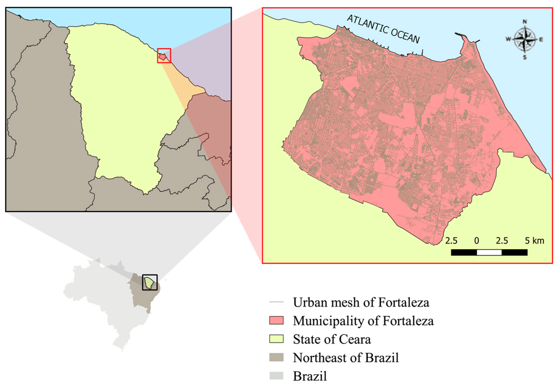
3. Study Area
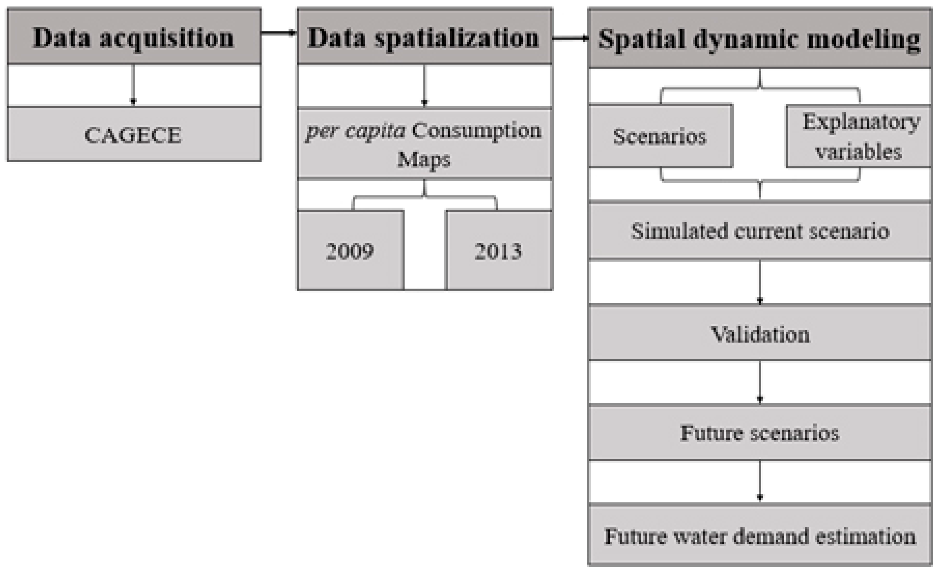
4. Data and Methods
4.1. Input Data for the Simulation Model
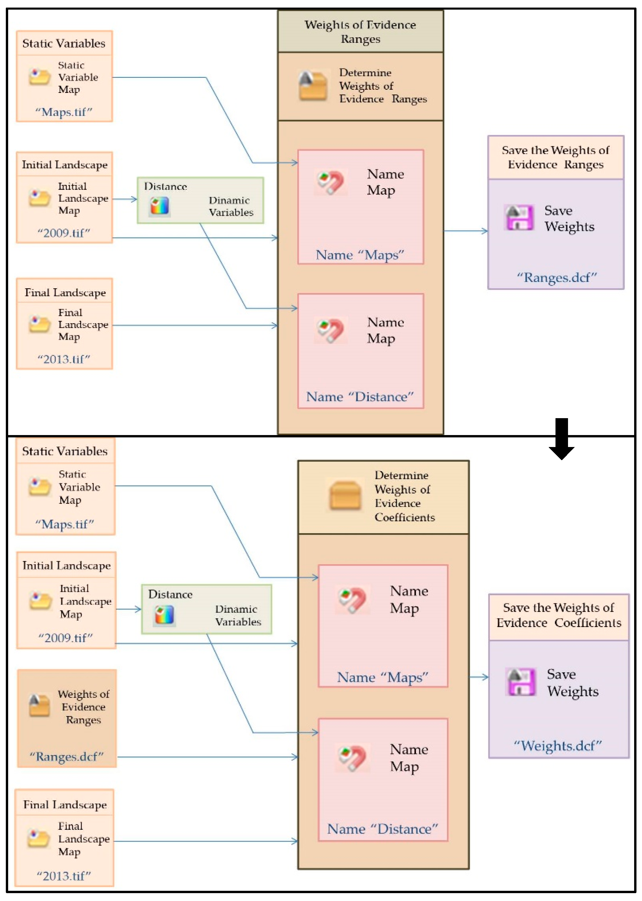
4.2. Model Calibration and Validation
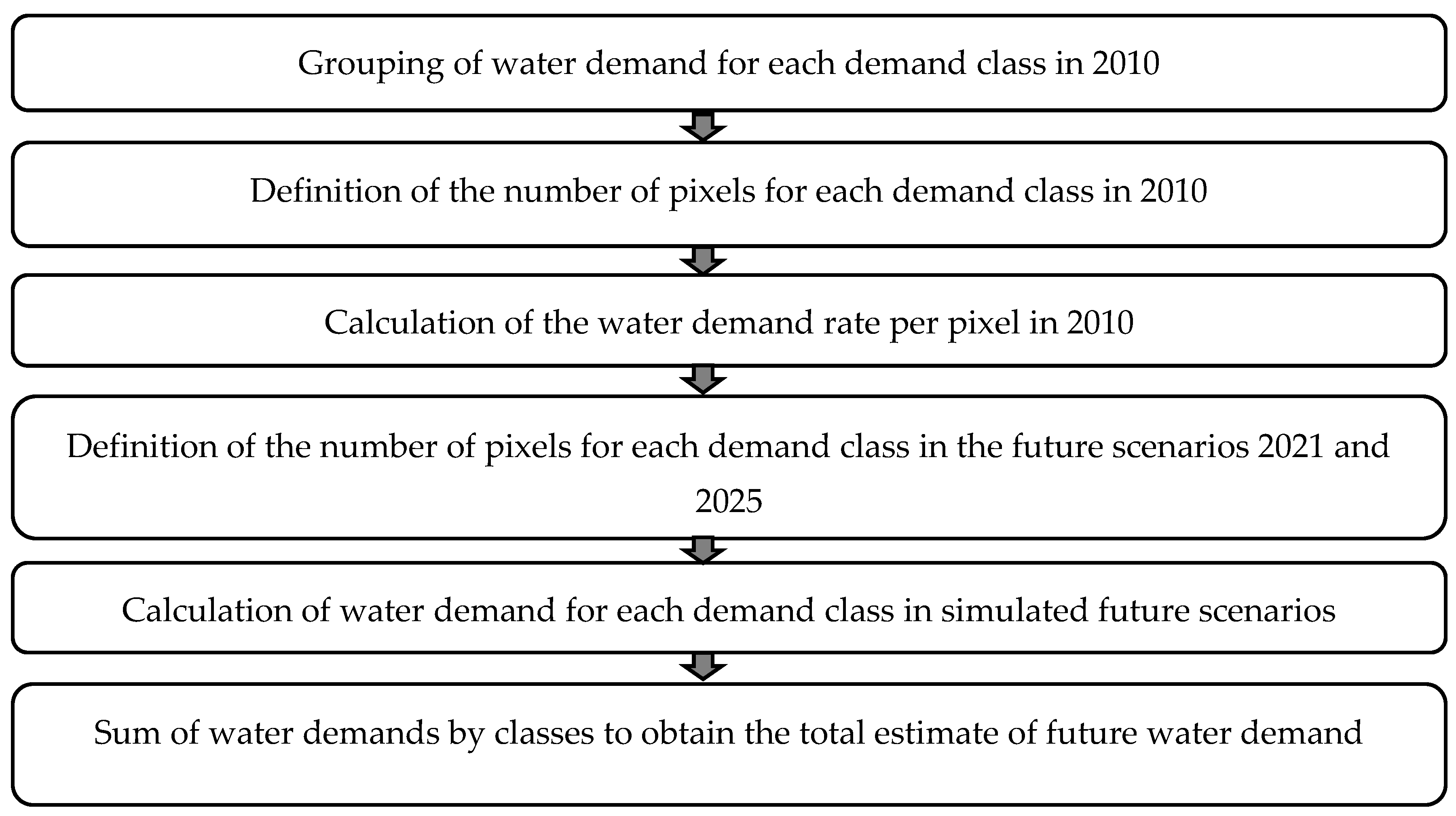
4.3. Estimation and Validation of Future Water Demands
5. Results
6. Conclusions
Author Contributions
Funding
Conflicts of Interest
References
- Sharma, S.K.; Vairavamoorthy, K. Urban water demand management: Prospects and challenges for the developing countries. Water Environ. J. 2009, 23, 210–218. [Google Scholar] [CrossRef]
- Dias, D.M.; Martinez, C.B.; Libânio, M. Avaliação do impacto da variação da renda no consumo domiciliar de água. Eng. Sanit. Ambient. 2010, 15, 155–166. [Google Scholar] [CrossRef]
- Rodrigues, B.R.M.; Garcia, R.A. Avaliação dos principais aspectos associados ao consumo de água nos municípios de Minas Gerais e do Brasil. Cad. Do Leste 2017, 17, 46–59. [Google Scholar]
- Chaib, E.B.D.; Rodrigues, F.C.; Maia, B.H.; Nascimento, N.O. Avaliação do potencial de redução do consumo de água potável por meio da implantação de sistemas de aproveitamento de água de chuva em edificações unifamiliares. Rev. Bras. Recur. Hídr. 2015, 20, 605–614. [Google Scholar] [CrossRef]
- Narchi, H. A demanda doméstica de água. Rev. DAE 1989, 49, 1–7. [Google Scholar]
- Fernandes Neto, M.L. Avaliação de Parâmetros Intervenientes no Consumo per Capita de Água: Estudo Para 96 Municípios do Estado de Minas Gerais. Master’s Thesis, Universidade Federal de Minas Gerais, Belo Horizonte, Brazil, 2003. [Google Scholar]
- Guedes, N.S.; Athayde Júnior, G.B.; Chaves, G.L.R. Avaliação do consumo per capita de água em municípios do Nordeste do Brasil. In Proceedings of the VII Congresso Brasileiro de Gestão Ambiental, Campina Grande, Brazil, 21–24 November 2016. [Google Scholar]
- Dias, D.M. Avaliação do Impacto da Renda Sobre o Consumo Hidrometrado de Água em Domicílios Residenciais Urbanos: Um Estudo de Caso Para Regiões de Belo Horizonte. Master’s Thesis, Universidade Federal de Minas Gerais, Belo Horizonte, Brazil, 2008. [Google Scholar]
- Figueres, C. Urban water management in the Middle East and Central Asia. In Proceedings of the 12th World Water Congress of IWRA, New Delhi, India, 22–25 November 2005. [Google Scholar]
- Rêgo, J.C.; Galvão, C.O.; Vieira, Z.M.C.L.; Ribeiro, M.M.R.; Albuquerque, J.P.T.; Souza, J.A. Atribuições e responsabilidades na gestão dos recursos hídricos—O caso do açude Epitácio Pessoa/ Boqueirão no Cariri paraibano. In Proceedings of the XX Simpósio Brasileiro de Recursos Hídricos, Bento Gonçalves, Rio Grande do Sul, Brazil, 17–22 November 2013. [Google Scholar]
- Meniconi, S.; Brunone, B.; Frisinghelli, M. On the role of minor branches, energy dissipation, and small defects in the transient response of transmission mains. Water 2018, 10, 187. [Google Scholar] [CrossRef]
- Rossetti, L.A.F.S.; Almeida, C.M.; Pinto, S.A.F. Análise de mudanças no uso do solo urbano e rural com aplicação de modelagem dinâmica espacial. In Proceedings of the XVI Simpósio Brasileiro de Sensoriamento Remoto, Foz do Iguaçu, Brazil, 13–18 April 2013. [Google Scholar]
- Granjeiro, E.L.A.; Rufino, I.A.A.; Barros-Filho, M.N. Estimativa e espacialização da demanda de água na cidade de Campina Grande/PB considerando o uso e a ocupação do solo: O caso do bairro do Catolé. In Proceedings of the XXI Simpósio Brasileiro de Recursos Hídricos, Brasília, Brazil, 22–27 November 2015. [Google Scholar]
- Yan, K.; Yang, M.-Z. Water demand forecast model of least squares support vector machine based on particle swarm optimization. MATEC Web Conf. 2018, 246, 9. [Google Scholar] [CrossRef][Green Version]
- Haque, M.M.; Rahman, A.; Hagare, D.; Chowdhury, R.K. A comparative assessment of variable selection methods in urban water demand forecasting. Water 2018, 10, 419. [Google Scholar] [CrossRef]
- Adamowski, J.F. Peak daily water demand forecast modeling using artificial neural networks. J. Water Resour. Plan. Manag. 2008, 134, 119–128. [Google Scholar] [CrossRef]
- Cosgrove, W.J.; Loucks, D.P. Water management: Current and future challenges and research directions. Water Resour. Res. 2015, 51, 4823–4839. [Google Scholar] [CrossRef]
- Suhartono, S.; Isnawati, S.; Salehah, N.A.; Prastyo, D.; Kuswanto, H.; Lee, M.H. Hybrid SSA-TSR-ARIMA for water demand forecasting. Int. J. Adv. Intell. Inform. 2018, 4, 238–250. [Google Scholar] [CrossRef]
- Giacomoni, M.H.; Berglund, E.Z. A complex adaptive simulation framework for evaluating adaptive demand management for urban water resources sustainability. J. Water Resour. Plan. Manag. 2015, 141, 1–12. [Google Scholar] [CrossRef]
- Shah, S.; Ben-Miled, Z.; Schaefer, R.; Berube, S. Differential learning for outliers: A case study of water demand prediction. Appl. Sci. 2018, 8, 2018. [Google Scholar] [CrossRef]
- Oliveira, L.M. Modelagem Dinâmica e Cenários Urbanos de Demanda de Água: Simulações em Campina Grande—PB. Master’s Thesis, Universidade Federal de Campina Grande, Campina Grande, Brazil, 2019. [Google Scholar]
- Votsis, A. Utilizing a cellular automaton model to explore the influence of coastal flood adaptation strategies on Helsinki’s urbanization patterns. Comput. Environ. Urban. Syst. 2017, 64, 344–355. [Google Scholar] [CrossRef]
- IBGE. Available online: https://www.ibge.gov.br/estatisticas-novoportal/sociais/populacao/9662-censo-demografico-2010.html?=&t=o-que-e (accessed on 5 June 2019).
- Secretaria Municipal de Meio Ambiente de Fortaleza. Plano Municipal de Saneamento Básico de Fortaleza Convênio de Cooperação Técnica Entre Companhia de Água e Esgoto do Ceará—CAGECE e Agência Reguladora de Fortaleza—ACFOR. Diagnóstico do Sistema de Esgotamento Sanitário Revisado; Secretaria Municipal de Meio Ambiente de Fortaleza: Fortaleza, Brazil, 2014; 280p.
- Silva, S.M.O.; Souza Filho, F.A.; Cid, D.A.C.; Aquino, S.H.S.; Xavier, L.C.P. Proposta de gestão integrada das águas urbanas como estratégia de promoção da segurança hídrica: O caso de Fortaleza. Eng. Sanit. Ambient. 2019, 24, 239–250. [Google Scholar] [CrossRef]
- Soares-Filho, B.S.; Rodrigues, H.O.; Costa, W.L. Modelagem de Dinâmica Ambiental com Dinamica EGO, 1st ed.; Centro de Sensoriamento Remoto/Universidade Federal de Minas Gerais: Belo Horizonte, Brazil, 2009; 116p. [Google Scholar]
- Soares-Filho, B.S.; Cerqueira, G.C.; Pennachin, C.L. DINAMICA—A stochastic cellular automata model designed to simulate the landscape dynamics in an Amazonian colonization frontier. Ecol. Model. 2002, 154, 217–235. [Google Scholar] [CrossRef]
- Bonham-Carter, G.F. Geographic Information Systems for Geoscientists: Modelling with GIS, 1st ed.; Pergamon: Ontário, ON, Canada, 1994; 398p. [Google Scholar]
- Almeida, C.M.; Gleriani, J.M.; Castejone, F.; Soares-Filho, B.S. Using neural networks and cellular automata for modelling intra-urban land-use dynamics. Int. J. Geogr. Inf. Sci. 2008, 22, 943–963. [Google Scholar] [CrossRef]
- Hagen-Zanker, A. Fuzzy set approach to assessing similarity of categorical maps. Int. J. Geogr. Inf. Sci. 2003, 17, 235–249. [Google Scholar] [CrossRef]
- IPLANFOR. Avaliação da Segurança Hídrica de Fortaleza, Instituto de Planejamento de Fortaleza: Fortaleza, Brazil. Available online: https://fortaleza2040.fortaleza.ce.gov.br/site/fortaleza-2040/publicacoes-do-projeto.2016 (accessed on 17 July 2020).
- Dantas, E.W.C. Programa de desenvolvimento do turismo no nordeste Brasileiro (1995–2005): PRODETUR—NE, o divisor de águas. In Turismo e Imobiliário Nas Metrópoles, 1st ed.; Dantas, E.W.C., Ferreira, A.L., Clementino, M.L.M., Eds.; Letra Capital: Rio de Janeiro, Brazil, 2010; Volume 1, pp. 35–54. [Google Scholar]
- Novaes, M.R.; Almeida, C.M.; Rudorff, B.F.T.; Aguiar, D.A. Cenários prognósticos baseados em modelagem dinâmica espacial para o manejo da colheita da cana-de-açúcar no estado de São Paulo. In Proceedings of the XV Simpósio Brasileiro de Sensoriamento Remoto, Curitiba, Brazil, 30 April–5 May 2011. [Google Scholar]
- Soares-Filho, B.S.; Rodrigues, H.; Follador, M. A hybrid analytical-heuristic method for calibrating land-use change models. Environ. Model. Softw. 2013, 43, 80–87. [Google Scholar] [CrossRef]


| Year | Consumer Category | Total | |||
|---|---|---|---|---|---|
| Residential | Commercial | Industrial | Public | ||
| 2009 | 106,478,863 | 6,835,526 | 3,476,270 | 4,346,633 | 121,137,292 |
| 87.9% | 5.6% | 2.9% | 3.6% | 100.0% | |
| 2010 | 115,284,964 | 7,569,662 | 3,809,749 | 4,731,477 | 131,395,852 |
| 87.7% | 5.8% | 2.9% | 3.6% | 100.0% | |
| 2011 | 113,630,513 | 7,820,580 | 3,905,774 | 4,565,486 | 129,922,353 |
| 87.5% | 6.0% | 3.0% | 3.5% | 100.0% | |
| 2012 | 116,080,193 | 8,304,057 | 4,893,166 | 4,974,884 | 134,252,300 |
| 86.5% | 6.2% | 3.6% | 3.7% | 100.0% | |
| 2013 | 125,176,439 | 9,297,287 | 4,860,388 | 5,061,548 | 144,395,662 |
| 86.7% | 6.4% | 3.4% | 3.5% | 100.0% | |
| 2014 | 119,355,633 | 8,429,656 | 4,401,631 | 5,039,227 | 137,226,147 |
| 87.0% | 6.1% | 3.2% | 3.7% | 100.0% | |
| 2015 | 112,524,506 | 8,039,630 | 4,024,938 | 4,890,770 | 129,479,844 |
| 86.9% | 6.2% | 3.1% | 3.8% | 100.0% | |
| 2016 | 104,562,627 | 7,056,524 | 4,730,244 | 4,573,362 | 120,922,757 |
| 86.5% | 5.8% | 3.9% | 3.8% | 100.0% | |
| 2017 | 90,209,543 | 6,409,223 | 3,954,204 | 5,742,885 | 106,315,855 |
| 84.9% | 6.0% | 3.7% | 5.4% | 100.0% | |
| Demand/Pixel Rate (2010) | |||
|---|---|---|---|
| Water Demand Classes | Number of Pixels | Water Demand (L/day) | Rate (L/day) |
| 1 | 19,061 | 2,284,771 | 119.87 |
| 2 | 283,244 | 245,652,412.1 | 867.28 |
| 3 | 23,023 | 284,515.54 | 1235.79 |
| 4 | 1036 | 155,493.1 | 1500.90 |
| 5 | 0 | 0 | 0 |
| 6 | 37 | 145,776.2 | 3939.90 |
| Class in 2009 | Class in 2013 | Change Percentage |
|---|---|---|
| 1 | 2 | 24.27% |
| 1 | 3 | 0.10% |
| 2 | 1 | 0.23% |
| 2 | 3 | 9.63% |
| 2 | 4 | 0.04% |
| 2 | 6 | 0.70% |
| 3 | 2 | 7.83% |
| 3 | 4 | 14.01% |
| 4 | 3 | 33.14% |
| Water Volume (m3) | Difference | |
|---|---|---|
| 2017 real | 2017 simulated | 2.76% |
| 285,810,829.3 | 293,700,133.9 | |
| Class in 2009 | Class in 2013 | Average Patch Size (ha) | Variance (ha) | Isometry |
|---|---|---|---|---|
| 1 | 2 | 14.64522059 | 23.46246257 | 1.328104457 |
| 1 | 3 | 2.1875 | 0 | 1.354679803 |
| 2 | 1 | 4.629807692 | 4.357588981 | 1.226899778 |
| 2 | 3 | 35.65357143 | 83.71615399 | 1.363150969 |
| 2 | 4 | 4.78125 | 0.044194174 | 1.301474326 |
| 2 | 6 | 45.515625 | 80.89871778 | 1.386848548 |
| 3 | 2 | 6.279411765 | 4.821274349 | 1.257982941 |
| 3 | 4 | 16.95454545 | 37.1232648 | 1.361264205 |
| 4 | 3 | 4.895833333 | 5.091480834 | 1.327692808 |
| Validation for 2015 (m3) | Difference | |
|---|---|---|
| Simulated | Observed | 2.38% |
| 288,422,145.4 | 281,706,099.5 | |
© 2020 by the authors. Licensee MDPI, Basel, Switzerland. This article is an open access article distributed under the terms and conditions of the Creative Commons Attribution (CC BY) license (http://creativecommons.org/licenses/by/4.0/).
Share and Cite
Marques de Oliveira, L.; Maria Oliveira da Silva, S.; de Assis de Souza Filho, F.; Maria Nunes Carvalho, T.; Locarno Frota, R. Forecasting Urban Water Demand Using Cellular Automata. Water 2020, 12, 2038. https://doi.org/10.3390/w12072038
Marques de Oliveira L, Maria Oliveira da Silva S, de Assis de Souza Filho F, Maria Nunes Carvalho T, Locarno Frota R. Forecasting Urban Water Demand Using Cellular Automata. Water. 2020; 12(7):2038. https://doi.org/10.3390/w12072038
Chicago/Turabian StyleMarques de Oliveira, Laís, Samíria Maria Oliveira da Silva, Francisco de Assis de Souza Filho, Taís Maria Nunes Carvalho, and Renata Locarno Frota. 2020. "Forecasting Urban Water Demand Using Cellular Automata" Water 12, no. 7: 2038. https://doi.org/10.3390/w12072038
APA StyleMarques de Oliveira, L., Maria Oliveira da Silva, S., de Assis de Souza Filho, F., Maria Nunes Carvalho, T., & Locarno Frota, R. (2020). Forecasting Urban Water Demand Using Cellular Automata. Water, 12(7), 2038. https://doi.org/10.3390/w12072038