1. Introduction
Precipitation constitutes spatially and temporally the most highly variable atmospheric parameter [
1]. Traditional rain gauges serve a direct way of measuring local precipitation amounts [
2] and yield the longest available quantified records of them [
3]. Rain gauge locations do not typically follow any regular spatial pattern, rather spatial distribution of the gauges on almost any scale is highly inhomogeneous and changes frequently as old gauges are decommissioned or relocated, or new gauges are added [
4]. For water resources studies, local precipitation amounts are rarely sufficient as the water balance of a catchment requires an areal amount obtained from several local measurements, most frequently via different geostatistical [
5,
6,
7,
8] but sometimes even artificial intelligence [
9] or machine learning [
10] methods. New, alternative ways of precipitation observations (i.e., radar and satellite-based) present ever broader coverage and spatiotemporal resolution [
2,
11]; however, they cannot substitute for long-term records (mostly rain gauge-based) of precipitation that are crucial in understanding (and gauging the extent of) the ongoing climate change [
11] with its multifaceted consequences, such as encountered in water resources management (e.g., flood forecasting/protection, water-storage reservoir operations, water supply, drought early warning systems, etc.) [
12]. Precipitation not only forms one of the most important drivers in weather and climate studies [
2] but it does so in hydrological, hydrogeological [
13,
14,
15], hydro-meteorological and water resources investigations as well [
16]. Due to its crucial role in these areas and its pivotal position in the global hydrological cycle in general [
17], any approach that can help with its estimation in the lack of measured values on any spatial and temporal scale must be highly valuable (see the rapid expansion of satellite-based precipitation estimation products in e.g., [
11]), especially so if it can yield the same long-term temporal coverage as rain gauges do.
By the recently witnessed fast improvements in complementary-relationship (CR) based evapotranspiration (ET) estimation methods [
18,
19,
20], it has now become possible to obtain ET rates (on a temporal resolution of daily to monthly and at a typical spatial scale of ~1 km
2 and up) with a high accuracy from a minimal number of generally available atmospheric/radiative data (i.e., air- and dew-point temperature, wind speed, net surface radiation) and in a calibration-free manner [
21,
22,
23,
24].
The current catchment-scale annual precipitation estimation method employs a calibration-free version [
21] of the generalized complementary relationship (from now on GCR17) for obtaining monthly ET rates that subsequently are aggregated into annual values to be used in an inverted simplified water balance equation with the help of annual streamflow discharge values. In recent studies by Ma and Szilagyi [
23] and Ma et al. [
24] the GCR17 outperformed other (altogether eight) global mainstream gridded ET products (all of which also require precipitation to derive their ET rates, making them inadequate for the present purpose) over China and the conterminous United States, making it a natural candidate to perform the proposed water-balance based precipitation estimation. Since GCR17 employs a minimal number of generally available atmospheric/radiation (net surface radiation can be derived from more commonly available solar radiation) data of typically extended temporal coverage in addition to its calibration-free nature, it is able to provide similarly long annual precipitation time series (stream discharge measurements permitting), crucial in climate change studies for the detection of any modifications in tendencies and variability. As the proposed precipitation estimation method employs atmospheric variables with suppressed spatial variability (due to turbulent mixing of water vapor and heat content) in comparison with that in precipitation, plus it works on the watershed scale (the catchment acting as a natural spatial integrator for stream discharge), it may also alleviate (i.e., a representative spatial average of ET by the CR can be obtained from fewer and more widely spaced measurement locations) some of the problems in spatial representativeness of local precipitation measurements.
2. Methods
Considering that the ET estimation method is absolutely crucial for the proposed calibration-free water-balance based precipitation estimation, it is important to describe it in enough detail to be easily applicable by future users. See Szilagyi et al. [
21], Ma and Szilagyi [
23] and Ma et al. [
24] for additional information on the method’s theoretical background and examples of its applications.
The nonlinear GCR of Brutsaert [
18] relates two dimensionless variables,
x =
Ew Ep−1 and
y =
E Ep−1 as
Here E (mm d−1) is the actual and Ep (mm d−1) the potential ET rate, i.e., the evapotranspiration rate of a small wet patch in a drying (i.e., not fully wet) environment, while Ew is the same Ep in a wet environment. In the latter case the small wet patch evaporates at the same rate as its wet environment, i.e., E = Ep = Ew.
Szilagyi et al. [
21] introduced a correction factor in the definition of
x to define
X = (
Epmax −
Ep) (
Epmax −
Ew)
−1x, by which Equation (1) keeps its original nonlinear form, i.e.,
Epmax in the definition of
X is the maximum value that
Ep can, in theory, achieve during a complete dry-out (i.e., when the moisture content of the air is close to zero) of the environment.
Ep is typically specified by the Penman equation [
25] as
where
Δ (hPa °C
−1) is the slope of the saturation vapor pressure curve at air temperature,
T (°C), and
γ the psychrometric constant (hPa °C
−1).
Rn and
G are net surface radiation and soil heat flux into the ground (the latter is typically negligible on a monthly scale) in water equivalent of mm d
−1, respectively.
e* and
e (=
e*(
Td)) are the saturation and actual vapor pressure of the air (hPa),
Td is the dew-point temperature, and
fu is a wind function, formulated [
26] as
where
u2 (m s
−1) is the 2-m horizontal wind speed.
The wet-environment ET rate,
Ew (mm d
−1), observed over a regionally extensive well-watered surface, is specified by the Priestley–Taylor [
27] equation
The dimensionless Priestley–Taylor coefficient,
α, in Equation (5) assumes values typically from the range of 1.1–1.32 [
28]. For large-scale model applications of gridded data, Szilagyi et al. [
21] proposed a novel method of assigning an appropriate value for
α without the need of any calibration.
Note that Equation (5) was derived for completely wet environments by Priestley and Taylor [
27], and therefore,
Δ should be evaluated at the wet-environment air temperature,
Tw (°C), instead of the typical, drying environment
T [
29,
30]. By making use of a mild vertical air temperature gradient [
29,
31,
32] observable in wet environments (as
Rn is consumed predominantly by the latent and not by sensible heat flux),
Tw can be approximated by the wet surface temperature,
Tws (°C). Note that
Tws may still be larger than the drying-environment
T when the air is close to saturation, but not
Tw, due to the cooling effect of evaporation, and in such cases the estimated value of
Tw should be capped by
T [
29,
33]. Szilagyi and Schepers [
34] demonstrated that
Tws is independent of areal extent, thus
Tws can be obtained by iteration from the Bowen ratio (
β), which is the ratio of sensible and latent heat fluxes [
35] of a small wet patch (assuming that available energy for the wet patch is close to that of the drying surface) for which the Penman equation is valid, i.e.,
Epmax can also be defined by the Penman equation considering that
e is negligible now, i.e.,
in which
Tdry (°C) is the dry-environment air temperature. The latter can be estimated from the adiabat of an air layer in contact with the drying surface under constant
Rn − G [
36], i.e.,
where
Twb (°C) is the wet-bulb temperature.
Twb is derived by another iteration of writing out the Bowen ratio for adiabatic changes [
29] as
Ma and Szilagyi [
23] can be referred to for (i) a graphical illustration of the saturation vapor pressure curve, and the different temperatures and related ET rates defined above; (ii) a brief description of how the CR evolved into Equation (2) over the past 50-some years; (iii) plots of selected historical CR functions over sample data, and; (iv) how assigning a value of
α is performed without resorting to any calibration. A sensitivity analysis of the GCR17 ET rates to its drivers are also found in Ma et al. [
24].
GCR17 (i.e., Equation (2)) was applied in a continuous monthly simulation over the 37-year period of 1979–2015 across the conterminous US, employing the 4-km spatial resolution parameter-elevation regressions on independent slopes model (PRISM [
37]) monthly air and dew-point temperature data. The 32-km North Atlantic Regional Reanalysis monthly surface net radiation and 10-m wind data [
38] were linearly interpolated onto the PRISM grid, while also employing a power transformation [
26] of the 10-m wind (
u10) values into
u2 (=
u10(2/10)
1/7), required by Equation (4). The GCR17-derived monthly ET rates were then aggregated into annual sums for application of the catchment water-balance equation.
Annual streamflow rates,
Q, (mm yr
−1) came from the United States Geological Survey (USGS) that divides the country into successively smaller hydrological units with a unique “hydrological unit code” (HUC) [
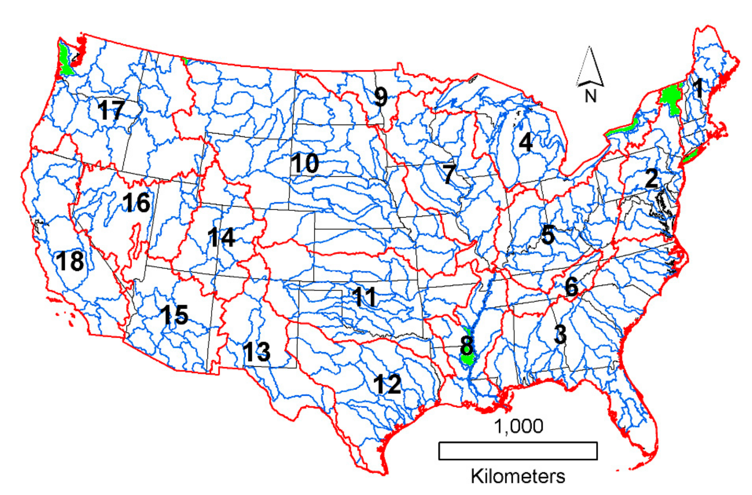
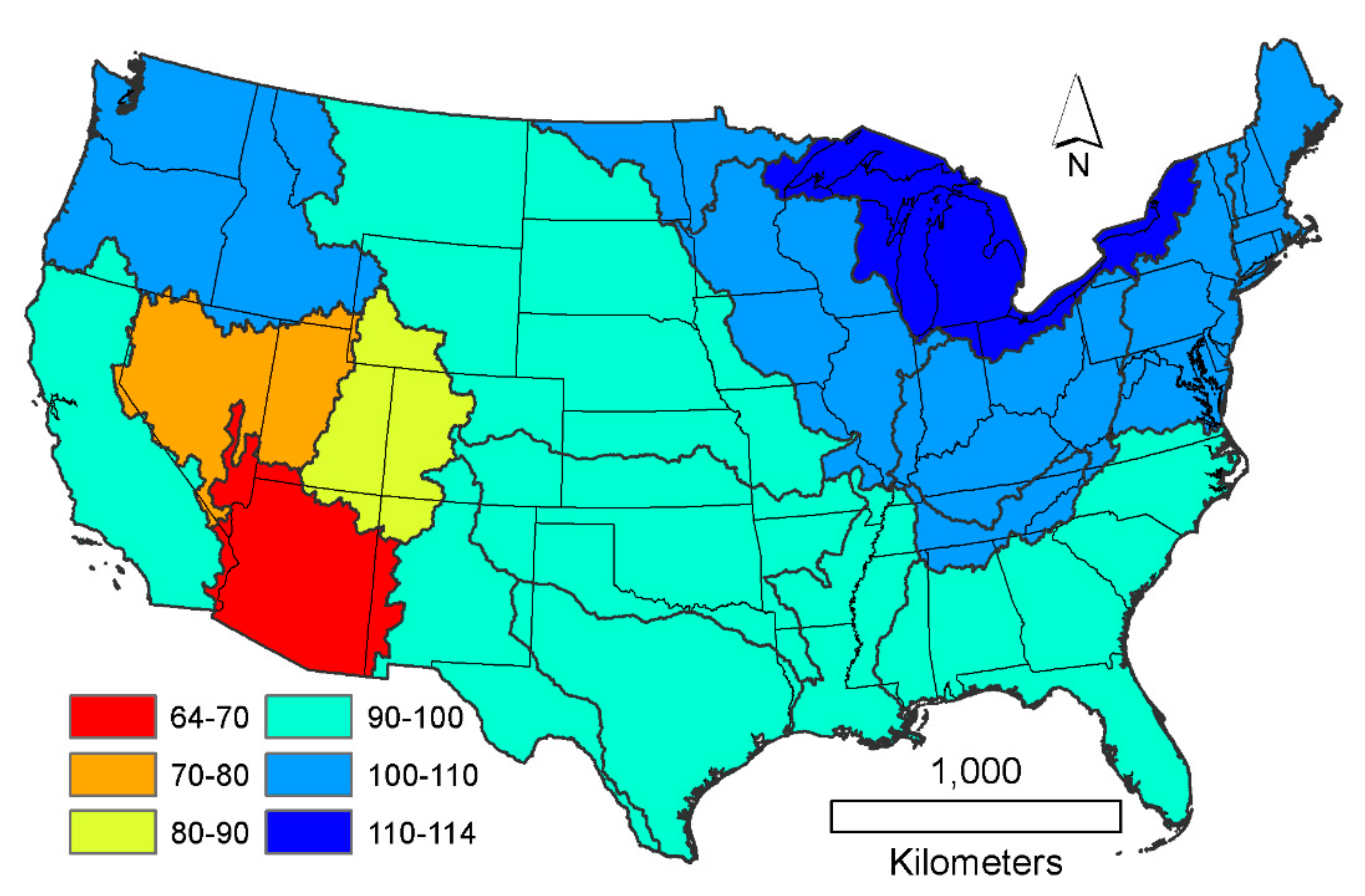
39] identifier. The conterminous US has 18 two-digit (HUC2) and 334 six-digit (HUC6) basins with a median area of about 4 × 10
5 and 2 × 10
4 km
2, respectively (
Figure 1).
Annual watershed or basin-scale ET rates are typically estimated by the lumped water-balance equation as
where
ΔS is the change in water storage over the basin/watershed, usually considered negligible at an annual (or longer) scale [
3] in comparison with the other two fluxes. Since ET (via averaging the PRISM-grid ET rate values of Equation (2) over the basin) and
Q are known, Equation (10) can be inverted for the estimation of annual precipitation over the basin/watershed as
Application of Equation (11) for smaller basins/watersheds may be affected by (i) significant inter-basin water exchanges [
33] and/or; (ii) operation of reservoirs with large (relative to mean streamflow) storage capacity [
40]. Altogether seven HUC6 basins (
Figure 1) were left out of the analysis because of their outlying (a difference in excess of 10% of the surrounding values)
Q and/or
P −
Q values.
While the Gravity Recovery and Climate Experiment (GRACE) data [
41] enables the estimation of basin-scale
ΔS [
42] in Equation (10), its available time-coverage (i.e., 2002–2018) is too short to allow for an improved (due to the typically large inter-annual variability of all the variables involved) estimation of linear tendencies, therefore Equation (11) was chosen to be applied over the entire available 1979–2015 data period. In fact, Ma and Szilagyi [
23] demonstrated that the statistical measures of the multiyear mean annual HUC2 and HUC6 GCR17 ET estimates were practically identical between the 1979–2015 and GRACE periods (for the latter including
ΔS), while those for the trend analysis worsened (Tables 2 and 3 in [
23]). In general, the shorter the data period the less reliable any trend analysis becomes as the weight of an individual observation (or its estimate) to the estimated trend increases. Including the GRACE
ΔS values only for the second part of the 1979–2015 period would make the precipitation estimates inhomogeneous, making the trend evaluations less reliable again.
The PRISM precipitation data was chosen for validation of the precipitation estimates because it was rigorously tested and validated by ground truth measurements [
37]. In a recent validation over a small mountainous research watershed, it yielded precipitation grid-values within 5% of gauging-station-derived data [
43].
3. Results
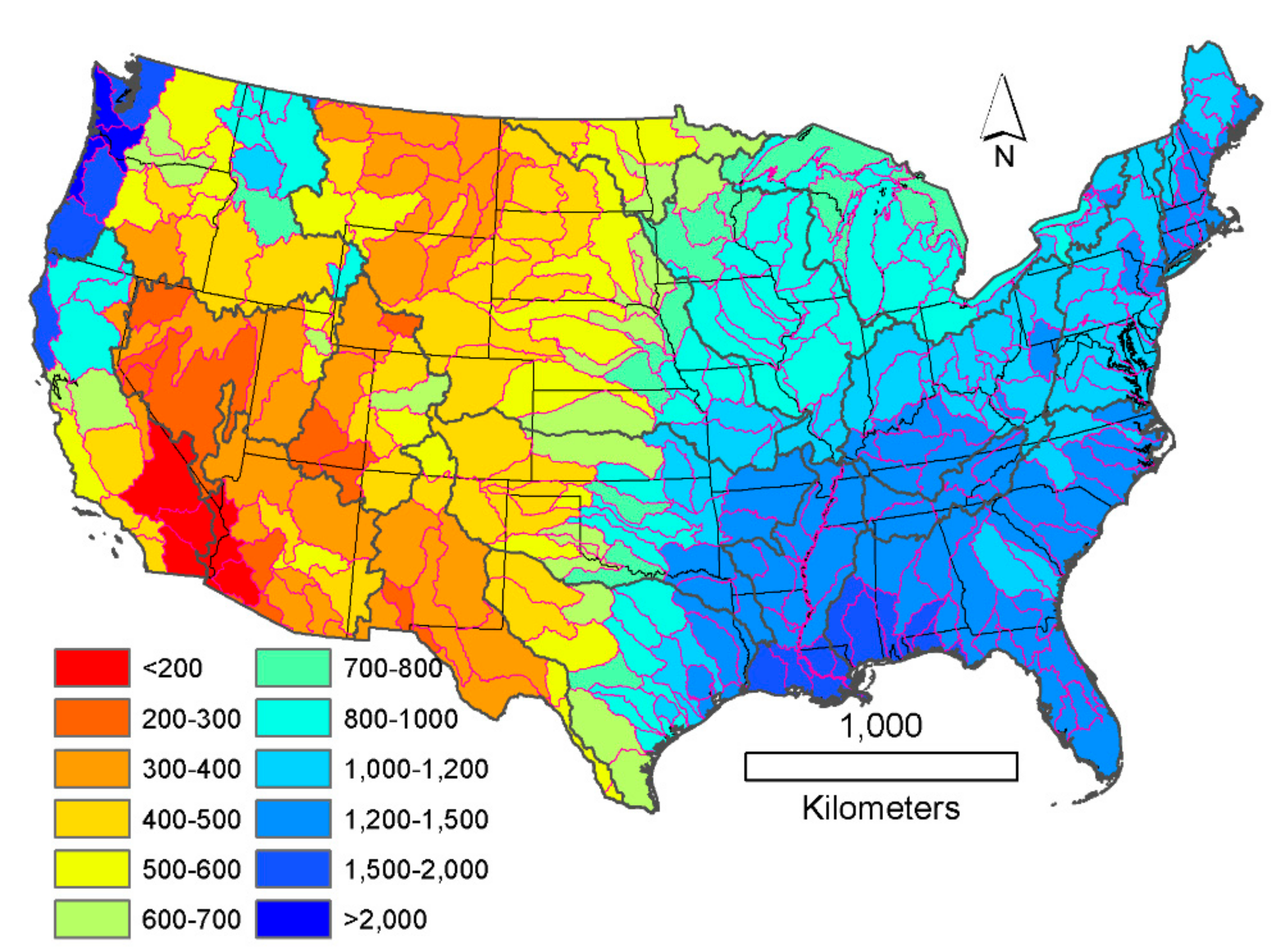
Spatial distribution of the mean annual (1979–2015) HUC6-averaged PRISM precipitation (
Figure 2) demonstrates the magnitude-wide range (i.e., below 200 to above 2000 mm yr
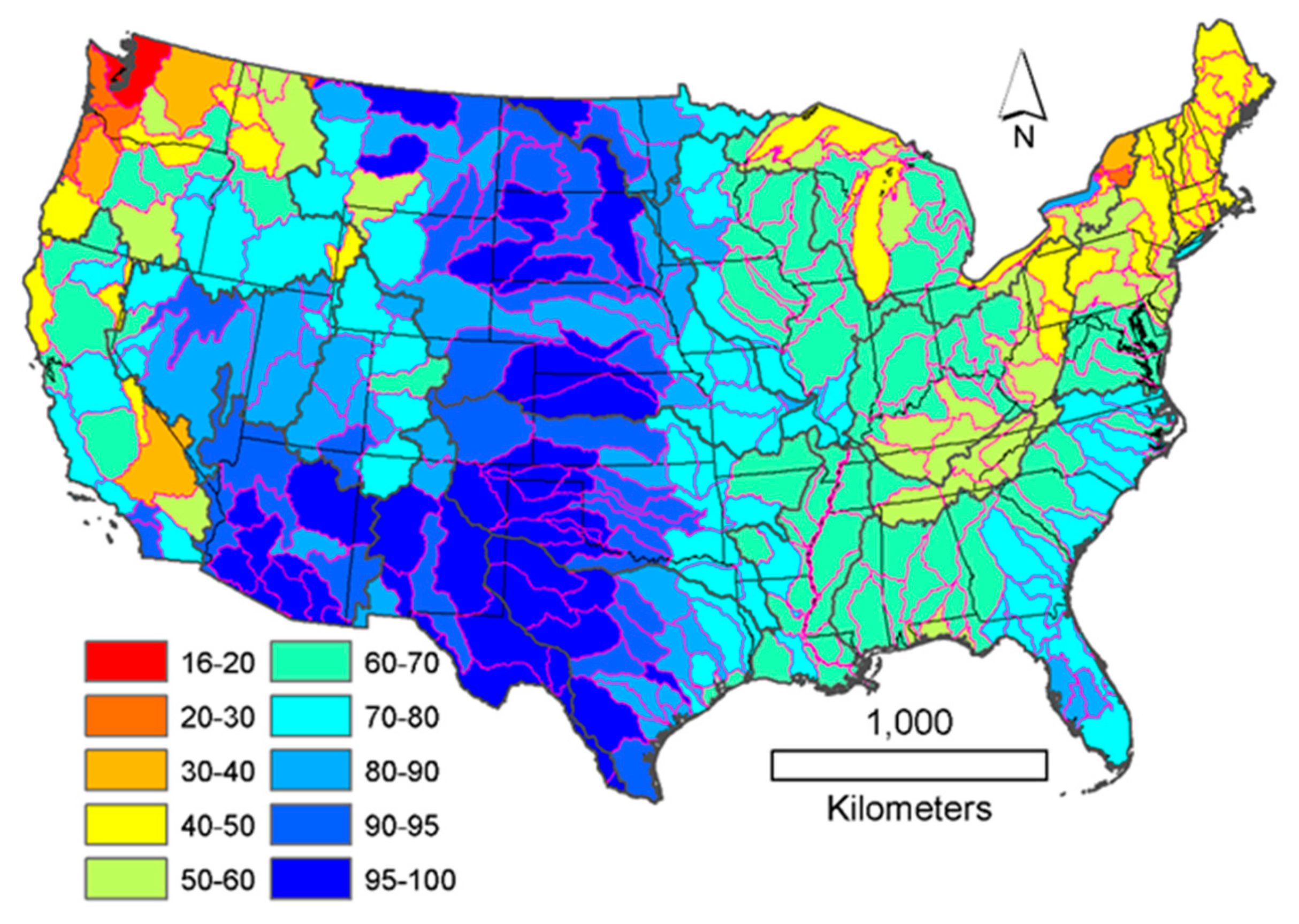
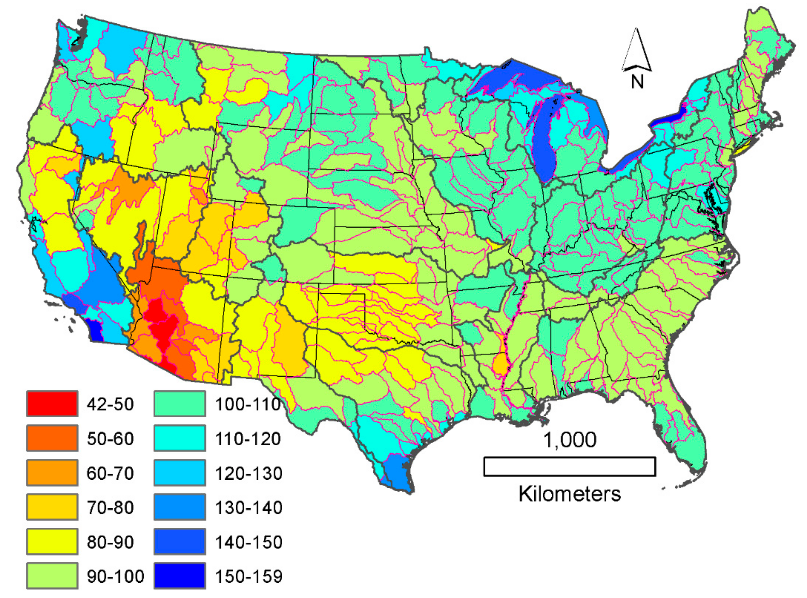
−1) found over the conterminous US, making it a perfect choice for testing the annual precipitation estimation method. Some irregularities—beside the above mentioned outliers in streamflow rates—further exist, visible in the spatial distribution of the ratio of water-balance ET and precipitation (ET ratio) values (
Figure 3). As a general rule, described by the Budyko curve [
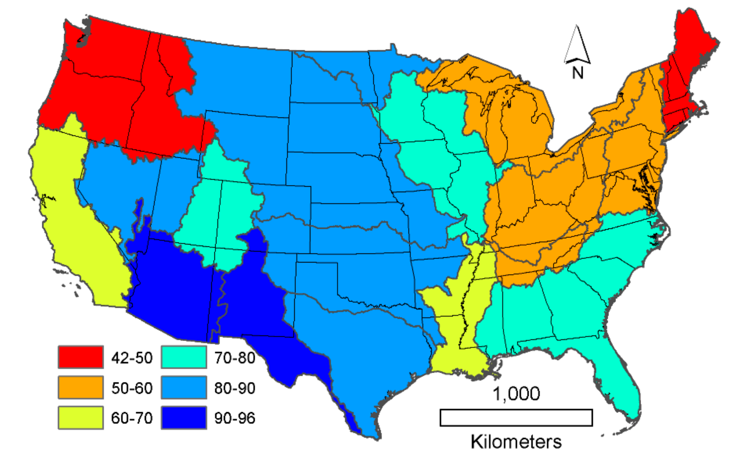
44], a larger proportion of the precipitation is expected to form ET in hot and arid regions compared to colder and humid ones. Yet, in southern California (within HUC2 #18), three HUC6 basins display unexpectedly low ET ratios (seen in yellow, orange and green colors). The cause may be either overestimation of the streamflow rate or underestimation of precipitation (or both). The irregularities, however, smooth out on the HUC2 scale (
Figure 4), confirming that accuracy of the water-balance equation (i.e., Equation (11)) generally improves with increasing spatial scales (at the simultaneous cost of reduced spatial/temporal variability among/within the HUC2 basins).
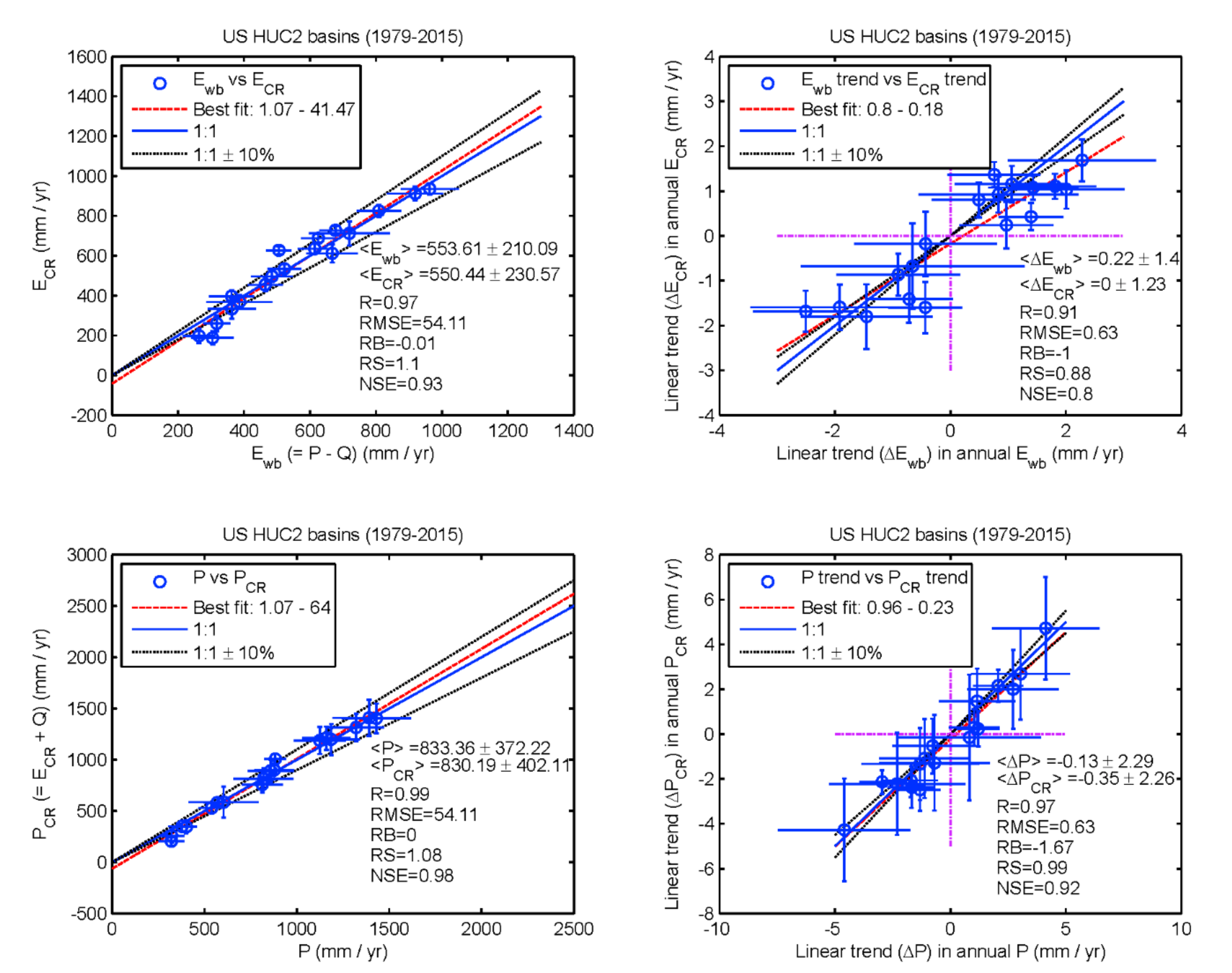
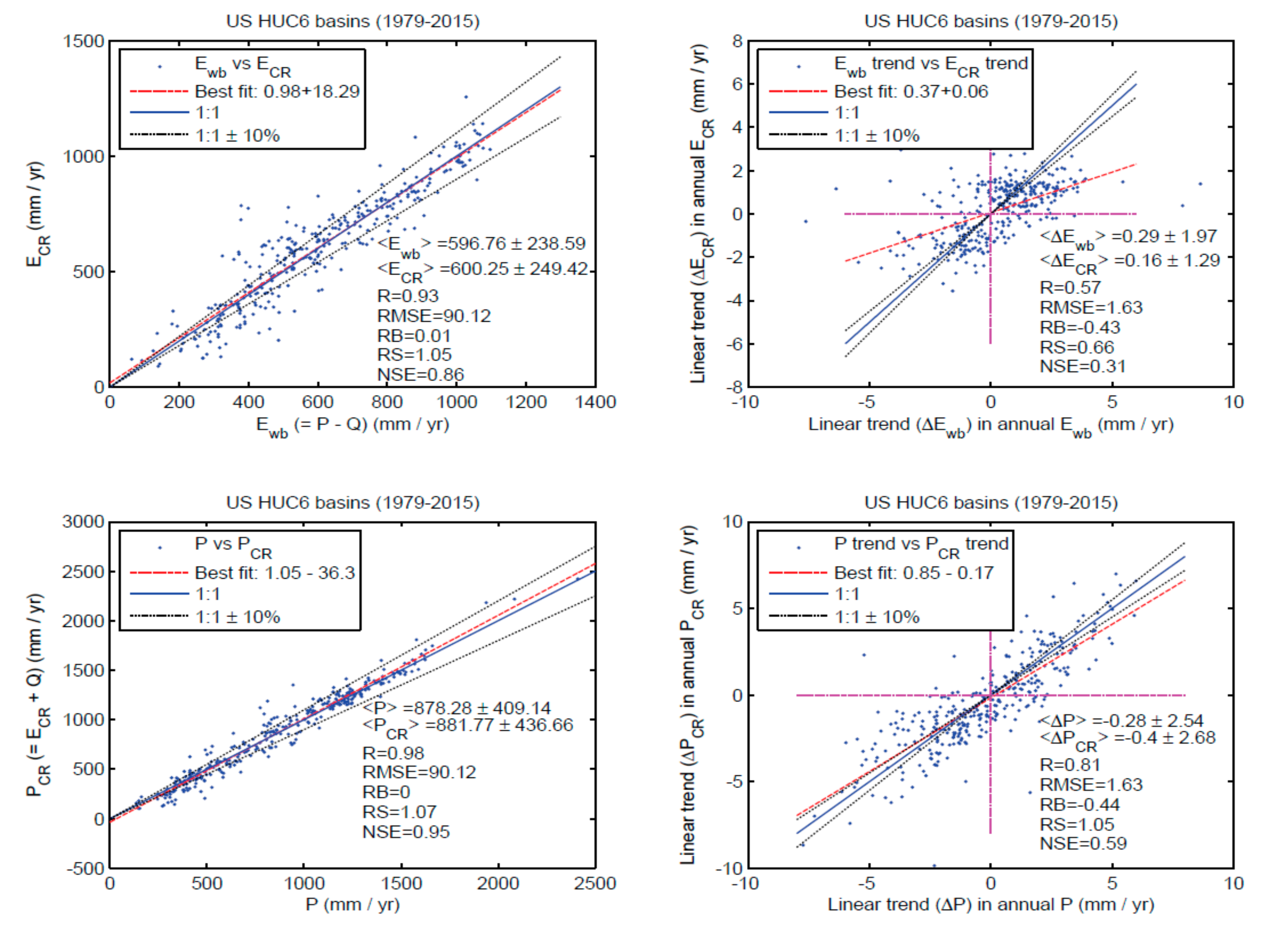
As the current water-balance based estimation of the annual precipitation rates depends so heavily on the ET estimates themselves, several statistical measures (also applied for
P) were employed to gauge that accuracy. At both HUC levels, first the arithmetic means (plus standard deviation) of the water-balance-derived and GCR17-estimated (a) mean (1979–2015) annual ET rates, as well as; (b) least-squares fitted linear tendencies in the annual ET values are obtained. Then the Pearson linear correlation coefficient (R), root-mean-squared-error (RMSE), relative bias (RB), ratio of the standard deviations (RS), and the Nash–Sutcliffe efficiency (NSE) are calculated for both (mean annual and linear tendency) values (see within the top panels of
Figure 5 and
Figure 6 and
Table 1). On top of these measures, linear regression plots for the mean annual ET rates and for the linear tendencies in annual values are also created (top panels in
Figure 5 and
Figure 6), including the best-fit line and a 10% error-band around the identity (1:1) line. In the HUC2 case, whiskers are also included in the regression plots (for HUC6 the large number of data points prevented it) depicting the standard deviation in the annual values for the long-term means and the standard error in the linear-tendency estimates.
The GCR17-derived ET rates yield unbiased estimates and strong linear correlations (R = 0.97 and 0.93 for the HUC2 and HUC6 cases, respectively) with the water-balance mean annual values, a similarly strong correlation with the water-balance linear tendencies (ΔE) on the HUC2 scale (R = 0.91), and a moderate one (R = 0.57) on the HUC6 level (both tendencies being underestimated but well within the error bounds). Except for HUC6 tendencies, the range of the estimated values are similar (RS is close to unity) and model efficiency is high (NSE ≥ 0.8). In general, GCR17 produces better mean annual ET and linear tendency estimates on the HUC2 level, at least partly due to the more accurate water-balance-derived values for reasons discussed above. Another reason is that on the smaller scale, surface properties vary to a larger degree between basins, not leaving enough distance (especially for elongated catchments perpendicular for the prevailing wind) for the atmosphere to fully adjust itself to those, sometimes abrupt (e.g., from dry-land to irrigated crops), changes and thus, not fully meeting the conditions required by the CR.
4. Discussions
Application of Equation (11) yielded surprisingly accurate, unbiased mean annual precipitation rates (sample mean, <
P >, of 830 ± 402 mm yr
−1 for HUC2 and 882 ± 437 mm yr
−1 for HUC6), well within 1% of the water-balance derived values (bottom panels of
Figure 5 and
Figure 6). Note that the two values differ because the basin means were not weighted by basin area. The basin-area-weighted long-term (1979–2015) precipitation average over the HUC2 basins is 790 ± 318 mm yr
−1 from PRISM values (mean annual cell values averaged over the HUC2 basins) and 789 ± 345 mm yr
−1 from Equation (11). In comparison, the arithmetic average (i.e., without previous averaging over the HUC2 basins) of the PRISM mean annual precipitation cell-values is 792 ± 451 mm yr
−1. The correlation coefficient values are very high (0.99 and 0.98 for HUC2 and HUC6, respectively) for the mean annual values, and remain similarly high (0.97) for the HUC2 trends (
ΔP) and somewhat weaker (0.81) for the HUC6 ones. These
R values mean that Equation (11) explains (i.e., the
R2 values equal the following numbers specified in percentages) 98, 96, 94, and 66% of the variance found among the basin-averaged (HUC2 and HUC6) mean annual precipitation rates (first two values) or among the relevant linear tendencies of the annual values (last two values). Note that the GCR17 ET rates alone can only explain 83, 72, 55, 24%, while streamflow rates explain 77, 70, 63, 45% of the variation found among the basin (HUC2 and HUC6) mean annual precipitation rates and among the linear tendencies.
The range of the estimated (mean and slope) values remain close (i.e., RS is within 0.99–1.08) to those found in the PRISM
P values. Model efficiency stays very high (NSE is within 0.92–0.98) for the means of both HUC levels and for the HUC2 trends, the latter slides somewhat (to 0.59) for HUC6 ones. In comparison with the ET case, the precipitation estimates either have the same accuracy in statistics (for RB and RMSE) or improved ones (R, RS, NSE) (see
Figure 5 and
Figure 6). This is possible due to the larger mean and standard deviation values found for
P in comparison with those for ET. The mean annual precipitation values can be estimated with about a 7% accuracy (RMSE/<
P >) on the HUC2 and with about a 10% one on the HUC6 level. Note that accuracy of the ET estimates is about 50% worse, i.e., 10% for HUC2 and 15% for HUC6.
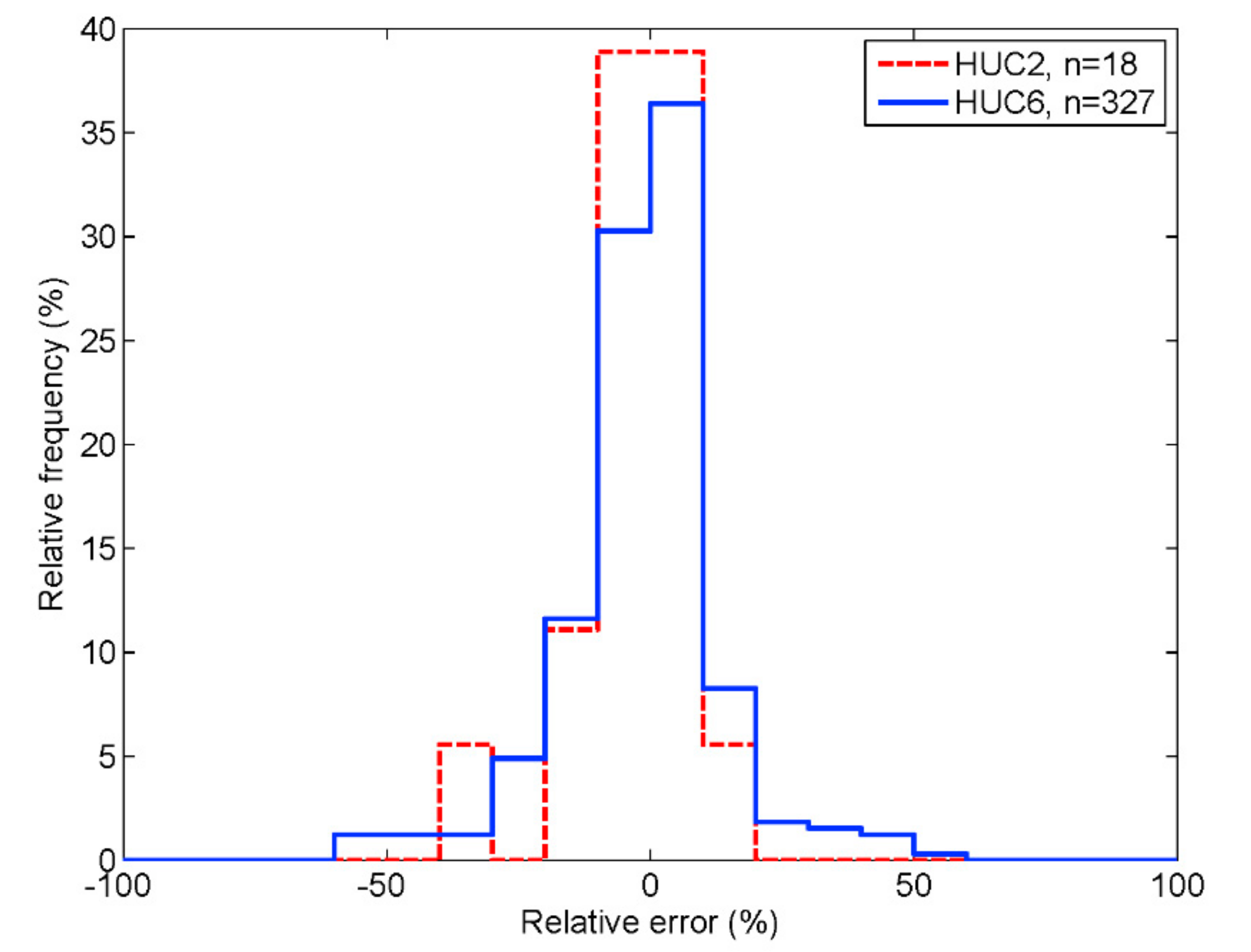
While the Equation (11)-derived mean annual precipitation rates are within 10% of the PRISM values (
Figure 7 and
Figure 8) in 15 out of 18 (=76%) HUC2 basins (the same ratio is 66% for HUC6), a relatively large (−36%) underestimation is found (
Figure 8) in the driest basin (Lower Colorado), resulting in a large negative
NSE value for the annual precipitation estimates. On the more detailed HUC6 level, the underestimation is obvious in the HUC6 basins (
Figure 9) of the Lower Colorado, but the exact opposite is observable in the California HUC2 basin. As such, a sharp switch from under- to overestimation over such a short distance cannot be found anywhere else within the conterminous US, and it is suspected that there may be a problem with the water-balance terms (i.e., precipitation and streamflow rate) in this south-western region. For example, Hanak et al. [
45] estimates that about 5.43 km
3 of water is being transferred from the Colorado River to California each year (which translates into an extra 13 mm of water when spread evenly over the area of California, and into about 18 mm missing from Arizona, both values proportionally larger as the affected area shrinks), which is then mostly used for crop irrigation in Southern California. This inter-state water transfer can reduce streamflow rates of the Lower Colorado basin, thus partially explaining—around 20% of—the precipitation undershoot by Equation (11) for the Lower-Colorado HUC2 basin. The irrigation-enhanced ET rates in Southern California will also boost the precipitation estimates of Equation (11) for the HUC6 basins there.
The Great Basin and the Upper Colorado HUC2 basins also display a significant underestimation of the mean annual precipitation rates in
Figure 8 and
Figure 10 due to similar underestimation of the ET rates [
21]. In these dry basins, local ET rates may vary significantly depending on elevation, slope aspect, and proximity to streams and/or shallow ground water. It is suspected that the CR cannot adequately respond to high-ET land patches due to fast mixing of the moisture-laden air of such dispersed areas with the surrounding drier air.
In the Great Lakes basin, the large overestimation is due to the fact that #4 of the HUC2 basins includes large parts of the Great Lakes (
Figure 1), which naturally enhance basin-wide ET rates via open water evaporation, significantly raising water vapor levels, which the CR picks up. The Great Lakes are also fed by other rivers from Canada, so the water balance is far from being closed in this case.
Probably the best feature of the precipitation estimates is that they can yield fairly reliable estimates for the sign (whether positive (increasing) or negative (decreasing)) of the linear trend. For the HUC2 basins, there is only one single basin with an incorrect sign (
Figure 5), and even then the water-balance tendency is small (8 ± 31 mm dec
−1), while its estimated value (−1.5 ± 28 mm dec
−1) is practically zero. For the HUC6 basins, the sign of trend estimate is correct in about 90% of the 327 basins considered (
Figure 6). As was shown before, the streamflow-rate trend only explains 63 (HUC2) and 45% of the trend variations found in basin precipitation, thus one cannot predict precipitation tendencies from observed streamflow tendencies alone.
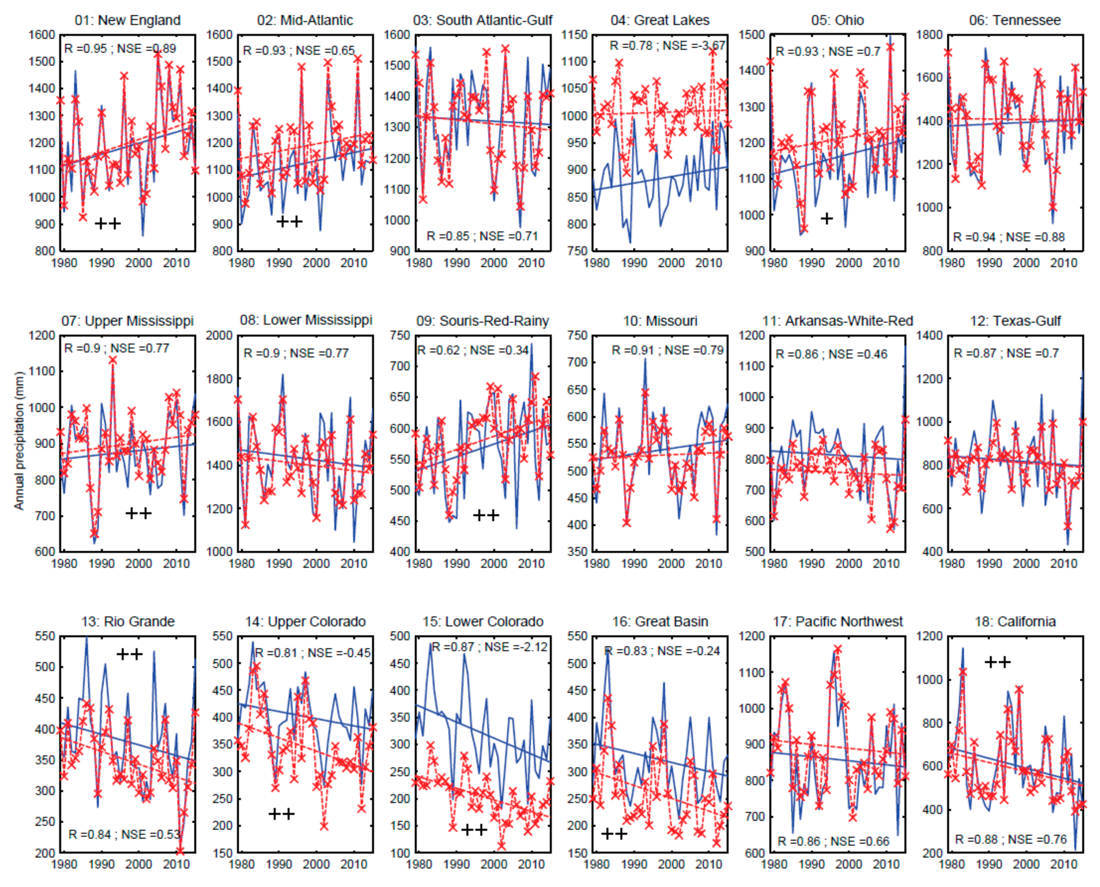
A graphical comparison of the annual PRISM and Equation (11)-derived precipitation and their trend values are seen in
Figure 10 for the 18 HUC2 basins. As seen, the water-balance estimates were able to capture significant trends 90% of the times without any false positives. The chosen 20% significance level made sure the test identified a trend when it was also obvious by the naked eye. The usual 5% significance level identifies only four trend cases (HUC2# 1, 5, 7, 15) for precipitation, which appears to be a substantial underestimation upon visual inspection of the graphs.
The R values of the practically unbiased (sample mean, <RB>, is a mere −3%) annual HUC2 precipitation estimates are typically over 0.8 (<R> = 0.86, which means that 74% of the PRISM
P inter-annual variability is explained by the estimates) with <RMSE> = 76.8 mm yr
−1 (i.e., the annual values in general are estimated with an accuracy better than 10%, as <
P> = 833 mm yr
−1), <RS> = 0.83, and median NSE value of 0.68. For NSE, the median is calculated rather than the mean due to the large (i.e., much larger than unity in absolute value) possible negative values (while NSE is limited by unity from above) when the difference in the means (in cases of significant over or underestimation) are large. The same measures for the HUC6 basins (
Table 1) are <R> = 0.82 (i.e., Equation (11) explains 2/3 of the precipitation inter-annual variability), <RB> = −1%, <RMSE> = 115.3 mm yr
−1, <RS> = 0.82, and the median of NSE is 0.47. These mean that the still unbiased annual precipitation estimates worsen on the HUC6 scale and precipitation can only be estimated with a 13% accuracy in general, and that the range of the annual estimates now is only 82% of that of the PRISM values. A general feature of the graphs in
Figure 10 is that even when the annual precipitation values are over- or underestimated, the trend-lines remain largely parallel on the HUC2 scale.
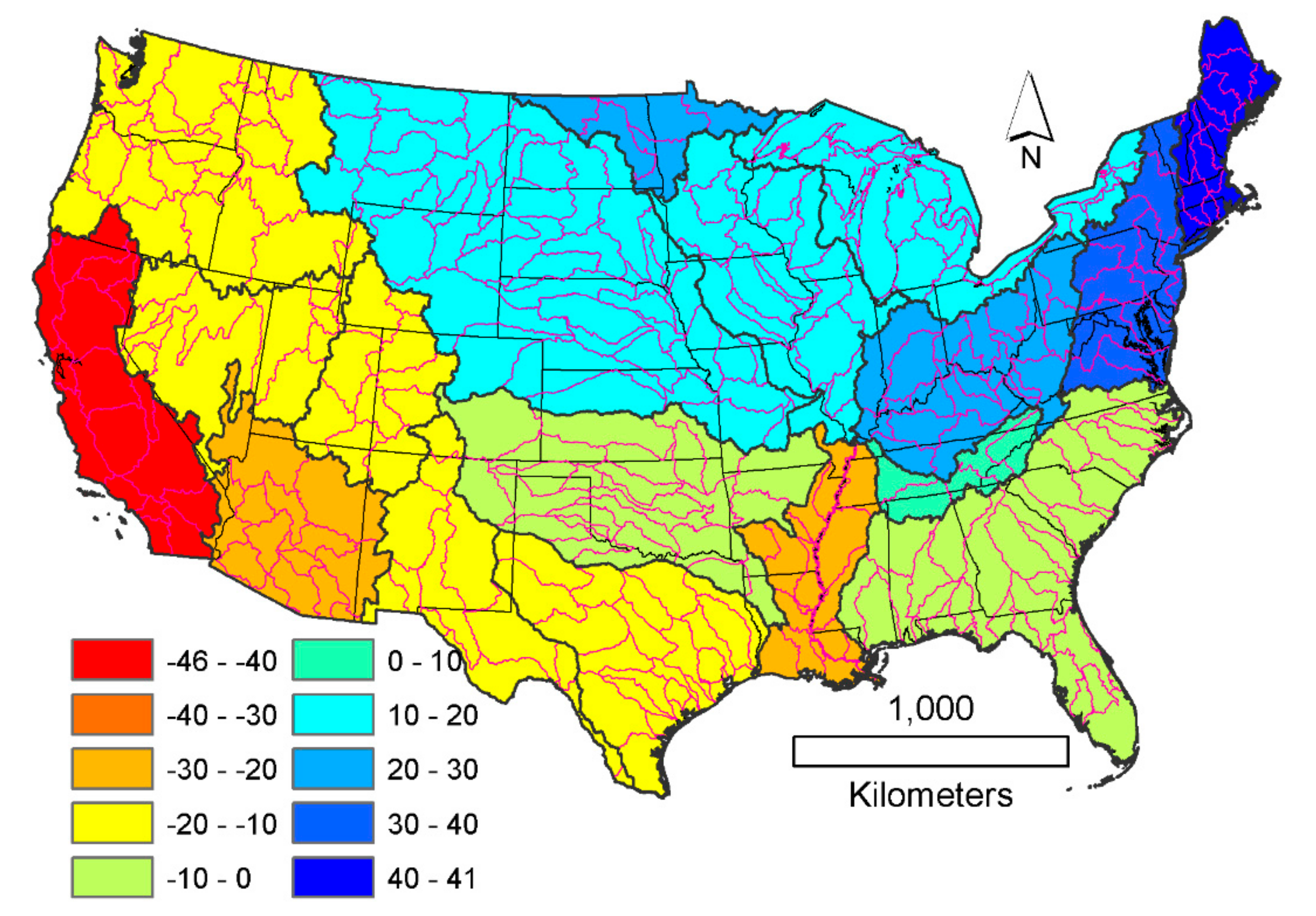
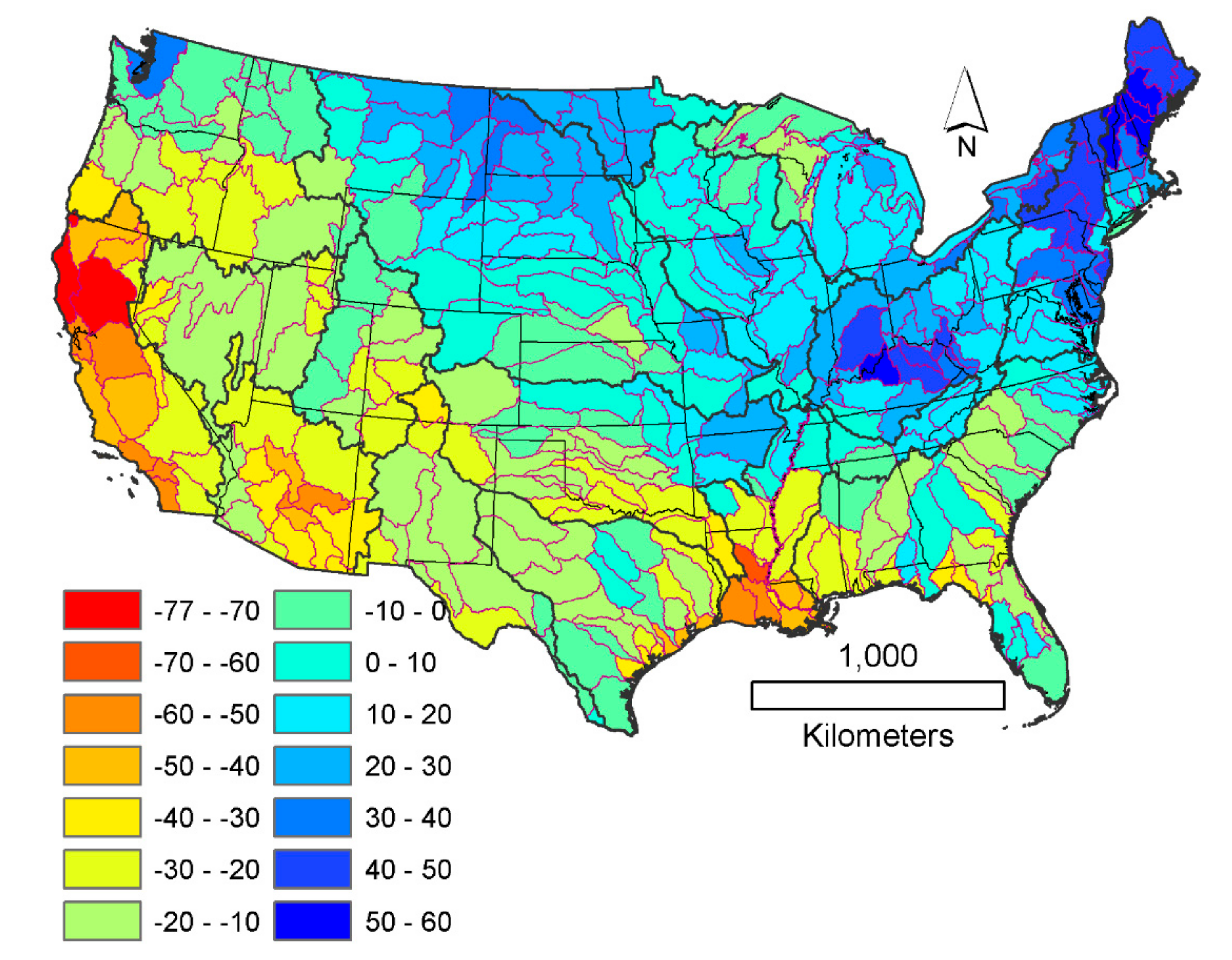
Figure 11 and
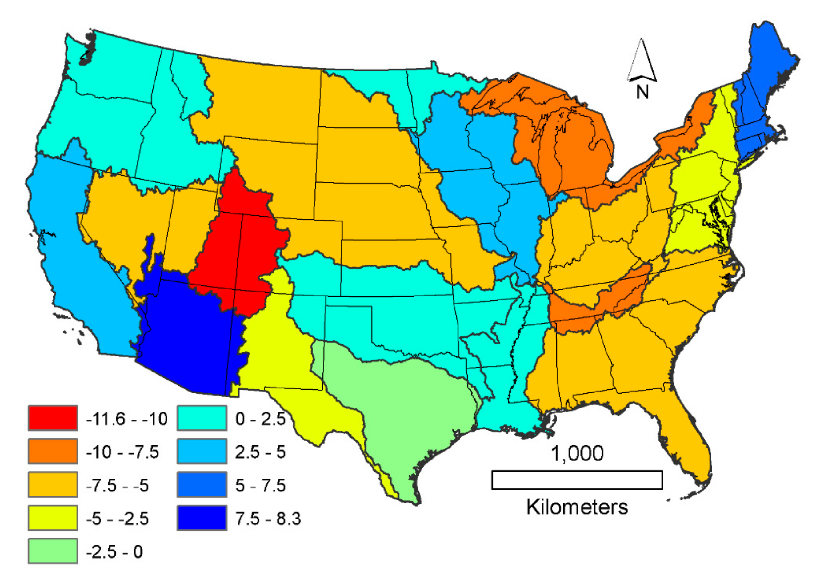
Figure 12 display the spatial distribution of the linear tendencies in PRISM annual (1979–2015) precipitation rates averaged over the HUC2 and HUC6 basins, respectively. The North-Central and North-Eastern US (about 40% of the total area of the conterminous US) exhibit increasing, while the rest, decreasing linear tendencies. The two extremes in trend on the HUC2 scale take place at the opposite ends of the country, i.e., in New England (41 mm dec
−1) and in California (−46 mm dec
−1), the latter a consequence of the mega-drought (
Figure 10) that took place between 2012 and 2015 [
33].
The Equation (11)-estimated linear tendencies are within ±10 mm dec
−1 of the PRISM
P tendency values in 17 HUC2 basins (i.e., 94%) out of the available 18 (
Figure 13 and
Figure 14). Note that for trends a relative error/bias, similar to the mean annual value estimation, cannot be correctly defined because such a value would approach infinity when the PRISM
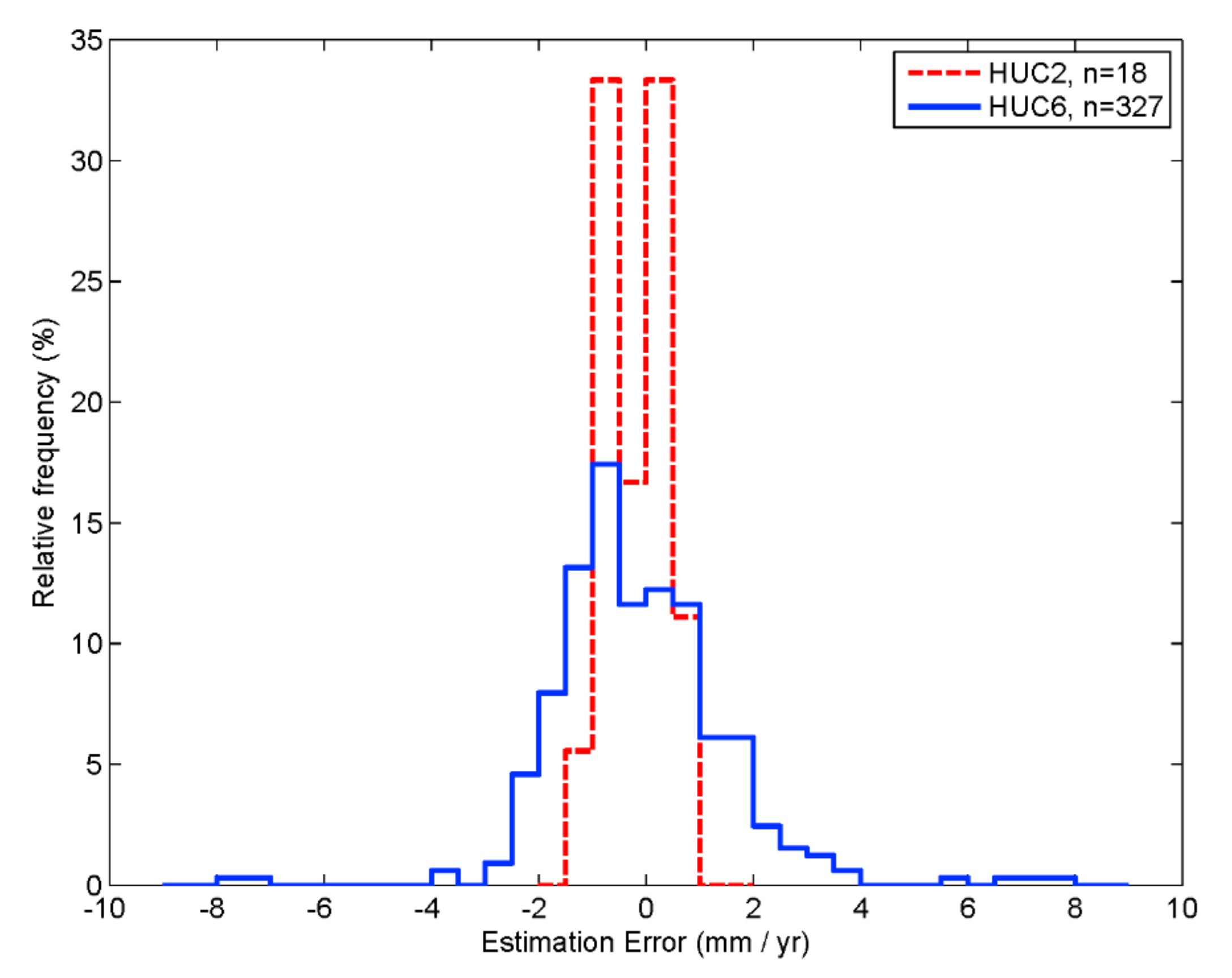
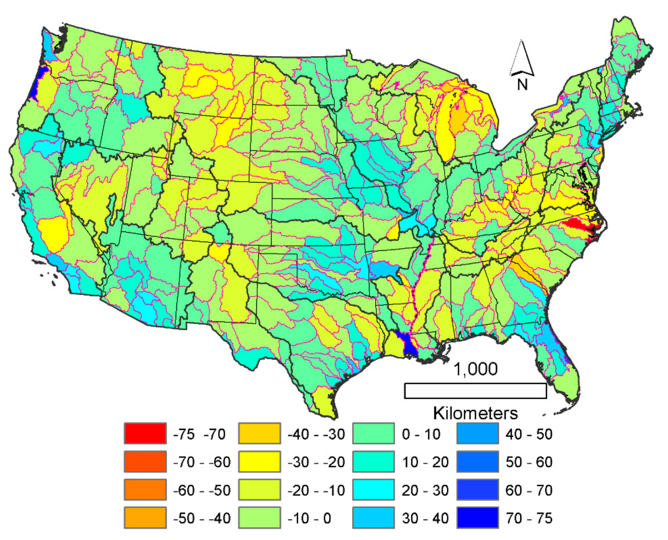
P trend approaches zero. On the HUC6 scale, accuracy drops with the observed significant range-increase (from about 20 in
Figure 14 to 150 mm dec
−1 in
Figure 15), and only 53% of the HUC6 basins are within the same limits (
Figure 13 and
Figure 15). Note that when the estimation error is opposite (happens in less than 10% of the basins for HUC6 and 6% for HUC2, see above) to—and its range is larger than—the observed trend, then there is a trend-change between predicted and observed values. Such cases, however, are rare.
5. Conclusions
In summary, it can be stated that annual precipitation rates can be estimated at least with an acceptable (see
Table 1 for the summary statistics) accuracy (sample means of R = 86 ± 8 (82 ± 10)%, RB = −3 ± 11 (−1 ± 15)% , RMSE = 77 ± 24 (115 ± 59) mm yr
−1, RS = 83 ± 14 (82 ± 20)%, and median NSE = 0.68 ± 1.2 (0.47 ± 2) for HUC2 (and HUC6 in parentheses) basins) for large (i.e., drainage area is larger than 10,000 km
2) watersheds with the help of a simplified water-balance equation in which monthly ET rates are estimated by the calibration-free generalized complementary relationship of Szilagyi et al. [
21]. The method yields improved estimates of the long-term (i.e., 30-year plus) mean annual watershed-scale precipitation rate (R ≥ 98%, RB = 0, RMSE ≤ 90 mm yr
−1, RS ≤ 108%, NSE ≥ 0.95) and the linear tendency of the annual values (R ≥ 81%, RMSE ≤ 1.63 mm yr
−1, RS ≤ 105%, NSE ≥ 0.59). Note that for trend values the relative bias (RB) is ill-defined (see above) and was left out from the evaluation summary.
The precipitation estimates improve with scale (
Table 1) partly because the requirements of the complementary relationship are more fully met on larger scales and partly because the simplified water balance equation itself improves with scale as inter-basin water transfers and inter-annual reservoir storage effects also diminish.
The unique advantage of the method is that annual precipitation rates can be estimated from few standard atmospheric/radiation (excluding precipitation) and stream discharge measurements in a calibration free manner, this latter meaning that it can be successfully applied even in cases when absolutely no information whatsoever exists about precipitation rates. The slight disadvantage of the method, however, is that setting the value of the Priestley–Taylor parameter requires gridded atmospheric/radiation data of a substantial spatial extent so that it would include at least periodically wet large surface areas. In cases when only the long-term precipitation trends are sought for, this impediment does not exist, since estimation of the linear tendency is not sensitive to the accuracy of the precipitation estimates (seen in
Figure 10), thus an assigned value of the Priestley–Taylor parameter from the typical range of 1.1–1.3 would be expected to work.
Performance of the method in this study was assessed using gridded input values, involving medium to large catchments. Further independent evaluations are needed on smaller watersheds and/or with scattered, ground-station input measurements. The method may especially be suited for applications over catchments where stream discharge and gridded input data are available but ground measurement of precipitation (for verification of the gridded precipitation) is missing or vastly hindered (by the limited number of gaging stations and/or varied topography) in its spatial representativeness.
