Article

Estimating Rainfall Design Values for the City of Oslo, Norway—Comparison of Methods and Quantification of Uncertainty

The Norwegian Meteorological Institute (MET Norway), Henrik Mohns plass 1, 0313 Oslo, Norway
*
Author to whom correspondence should be addressed.
Water 2020, 12(6), 1735; https://doi.org/10.3390/w12061735
Submission received: 30 April 2020 / Revised: 12 June 2020 / Accepted: 12 June 2020 / Published: 17 June 2020

Abstract

:
Due to its location, its old sewage system, and the channelling of rivers, Oslo is highly exposed to urban flooding. Thus, it is crucial to provide relevant and reliable information on extreme precipitation in the planning and design of infrastructure. Intensity-Duration-Frequency (IDF) curves are a frequently used tool for that purpose. However, the computational method for IDF curves in Norway was established over 45 years ago, and has not been further developed since. In our study, we show that the current method of fitting a Gumbel distribution to the highest precipitation events is not able to reflect the return values for the long return periods. Instead, we introduce the fitting of a Generalised Extreme Value (GEV) distribution for annual maximum precipitation in two different ways, using (a) a modified Maximum Likelihood estimation and (b) Bayesian inference. The comparison of the two methods for 14 stations in and around Oslo reveals that the estimated median return values are very similar, but the Bayesian method provides upper credible interval boundaries that are considerably higher. Two different goodness-of-fit tests favour the Bayesian method; thus, we suggest using the Bayesian inference for estimating IDF curves for the Oslo area.

1. Introduction

Around midnight on 4 August 2019, an intense thunderstorm surprised the forecasters at the Norwegian MET office (MET Norway) and the population of Oslo city. The thunderstorm divided the city into two, with dry conditions in the west and intense rainfall in the east. The return values for the shortest durations were estimated to exceed the 200-year level, resulting in urban flooding and a large amount of damage to property and infrastructure. Such events have become quite common in the southern part of Norway, partly due to an increase in the frequency and intensity of short-duration rainfall [1], and partly due to urbanisation and vulnerable infrastructure.
Norway has a complex topography, with a long coastline to the west. The encounter between cold Arctic air masses and warm humid air from the South gives rise to large frontal systems. The location at the end of the North Atlantic extratropical cyclones track (e.g., [2,3]) brings large and frequent storms, particularly during fall and winter, resulting in extreme rainfall and consequent flooding. Precipitation is further enhanced through orographic lifting as storms move inland and hit the mountains. Along the coast in the South, convective rainfall during summer can become quite intense, leading to flash floods in urban areas, as during the event on 4 August 2019. The different precipitation processes create large heterogeneities in extremes for different durations in different parts of Norway [1,4,5], and statistics will consequently be representative only for small regions.
Extreme precipitation and flooding can also trigger slides and avalanches, particularly affecting transport infrastructure and small communities near mountains (e.g., [6]). Costs associated with these natural hazards are large and are expected to increase with a changing climate [7]. In a green paper from the Norwegian government [8], the cost of damage caused by urban stormwater in Norway was estimated to be between 130 and 300 million euros per year. The same green paper reports that 60% of Norwegian municipalities had inadequate stormwater capacity for projected future precipitation, and lacked local competence, tools, and procedures for sustainable management of urban stormwater. The importance of high-quality and local precipitation statistics for proper infrastructure design and climate adaptation is therefore obvious.
Oslo, the capital of Norway, is situated at the northern end of Oslofjord, surrounded by hills and mountains. A combination of orography, a relatively large degree of urbanisation, old pipes, and natural river systems being closed in pipes back in time, makes Oslo highly exposed to urban flooding. Urban flooding events, often as a result of intense rainfall associated with convective conditions during summer, can close down traffic and cause damage to cellars and infrastructure [9].
Intensity-Duration-Frequency (IDF) curves [10] present short-duration precipitation statistics for different durations and frequencies (often in terms of return periods in years). IDF curves are a common tool in the planning and design of infrastructure, such as roads and railways and sustainable drainage systems. The computation of IDF values and their practical use differs quite a lot between different countries. The most frequently used methods include fitting the Generalised Extreme Value (GEV) [11] distribution to block maxima—usually annual maximum precipitation—or fitting the Generalised Pareto distribution [12] to Peak-Over-Threshold events. Olsson et al. [13] applied both methods in a regionalisation of short-duration extreme rainfall over Sweden. They proposed four regional IDF curves, using the station-year method to combine time series from all stations within each cluster. In Belgium and the Netherlands, the relatively flat terrain allows for the use of radar data in the estimation of spatially continuous IDF values (e.g., [14]). In Switzerland, the Federal Office of Meteorology and Climatology (MeteoSwiss) uses a Bayesian framework to fit the GEV distribution to annual maximum precipitation [15]. The results are presented in a web portal (http://climate-extremes.ch) where so-called intensity diagrams are shown, along with further results and information. In [16], IDF curves were computed for the province of Québec in Canada using the standard parameter estimation methods and the Bayesian approach for the GEV distribution. They suggest working with the Bayesian approach as it implicitly includes an uncertainty estimation.
Although none of the methods clearly outperform all the others, the literature suggests that the availability of precipitation data strongly guides the choice of method for estimating IDF values. Here, we focus on the GEV distribution, which is described by the three parameters: location ( μ ) , scale ( σ ) , and shape ( ξ ) . The shape parameter describes the tail of the distribution and influences, to a large degree, the estimates for long return periods [17]. It is also particularly hard to estimate, and has been scrutinised and discussed in the literature. Depending on ξ , the fitted distribution converges to one of three types (defined according to the convention used in [17]): Type I/Gumbel/EV1 ( ξ = 0 ) , Type II/Fréchet/EV2 ( ξ > 0 ) , and Type III/Weibull/EV3 ( ξ < 0 ) . Analysing a large global data set of 15,127 station series, Papalexiou and Koutsoyiannis [18] set out to answer which of the three cases of the GEV distribution annual maximum daily precipitation belongs to. They concluded that daily annual maxima follow a Type II distribution ( ξ > 0 ) worldwide, but the geographical location may affect ξ , and long time series are needed for reliable estimates. Koutsoyiannis [19,20], amongst others, found that the Gumbel distribution ( ξ = 0 ) most likely underestimates the largest precipitation extremes. For Norway, Dyrrdal et al. [5] found that ξ is largely positive in the eastern part of Southern Norway, while negative values dominate in the western part. They suggest a dependence on dominating precipitation systems and orographic enhancement. This was supported by [21], who found evidence that ξ differed between Norway and other parts of the world, and that ξ decreased with elevation.
In this study, we seek to advance the estimation of IDF values, or design rainfall, in Norway using the case of Oslo city. The current Norwegian method for IDF estimation was developed about 45 years ago, fitting a Gumbel distribution to the N-highest measurements (N being the time-series length in years) (see [22,23,24,25]). As mentioned above, the Gumbel distribution most likely underestimates the largest extremes. Additionally, the increase in extreme hydrological events strengthens the importance of updating the methodology, as also shown for other locations (e.g., [26,27]). We therefore propose to abandon the Gumbel distribution, and introduce two methods of fitting the GEV distribution to annual maxima: a modified Maximum Likelihood (ML) estimation [28] and Bayesian inference (e.g., [16,29,30]). Following the findings of [5,21], and the fact that time series of sub-daily precipitation are mostly short, we introduce a prior distribution to constrain the ξ parameter of the GEV distribution. The two methods are evaluated by different scores to indicate a new national methodology for IDF estimations. Since the shape parameter, ξ , is particularly hard to estimate, we give extra attention to the estimates of this parameter. We further quantify the uncertainty of the new IDF estimates, which, until now, has been a shortcoming in Norway.
A secondary aim of our paper is to facilitate the harmonisation of station and gridded IDF values. In [4], a Bayesian hierarchical model was proposed for the estimation of return values for hourly rainfall on a 1 km2 × 1 km2 grid covering the Norwegian mainland. This method has later been used to compute return values for other durations (down to 10 min) to form IDF curves. These are presented along with IDF curves from station data (https://klimaservicesenter.no/faces/desktop/idf.xhtml), but are currently not recommended for use in planning and design.
The manuscript is structured as follows: In Section 2 we introduce the Norwegian measurements of sub-daily precipitation and describe the current and the two experimental methods for estimating IDF values in Norway. Further, we explain the steps of the analysis. Section 3 presents results from comparing the three methods and IDF values for different meteorological stations in Oslo, and we discuss these results in Section 4. Ultimately, we summarise and conclude in Section 5.

2. Materials and Methods

2.1. Data

2.1.1. Measurements

Measurements of rainfall intensity with tipping bucket pluviographs in Norway started in the late 1960s. In the years 1967 to 1985, stations were set up in and around Oslo, operated by the Norwegian Water Resources and Energy Directorate (NVE) or the respective municipalities, Oslo and Bærum, in cooperation with MET Norway. MET Norway supervised the installation of the pluviographs and ensured they were installed according to recommendations from the World Meteorological Organisation (WMO), and also performed quality control and stored all data. The Norwegian-produced pluviograph Plumatic, manufactured by Kongsberg Våpenfabrikk A/S, was initially the preferred instrument. The Plumatic had a measuring range of 0.2 m m precipitation and a time resolution of one minute. Since it had no heating, it operated only in the extended summer months, from mid-April to mid-October. In the late 1990s and the early 2000s, the Plumatic pluviographs were successively replaced by the Lambrecht 1518H3 tipping bucket pluviometer (Lambrecht meteo GmbH, Göttingen, Germany) at all locations. Today, all the stations referred to hereunder operate with a Lambrecht 1518H3 pluviometer. The Lambrecht has a measuring range of 0.1 m m precipitation and a time resolution of one minute. The accuracy is given at ± 2 % , with intensity correction to account for the loss of rain due to the time required for the bucket to tip.
We consider time series of 10 years to be an absolute minimum for calculating IDF values. In the general Oslo area, there are 14 tipping bucket pluviometers with time series exceeding 10 years. Twelve of these are located within the municipality of Oslo and two in Bærum, the closest municipality to the West. See Figure 1 for a map of the stations, including the station ID and height above sea level.
The period of operation and time-series length varies from station to station (see Table 1). Two sets of precipitation series were extracted from each station, using different data availability requirements depending on the IDF estimation method. Series of the highest N values serve as input to the current method (Section 2.2.1), N being the number of years each station has been operative without requirements on the completeness of the season, while series of annual maxima serve as input to the two experimental methods with requirements on season completeness, as described in Section 2.2.2. Thus, the number of seasons in Table 1 refers to the length of the two data sets. Of the 14 tipping bucket gauge stations, seven stations have been operated continuously since the startup date. The other seven have been out of operation for short or long periods. As an example, station 19510, Øvrevoll started measuring in 1967 and is still in operation (53 whole years), but due to frequent downtime, the actual number of seasons in operation is 38. None of the stations has been relocated.

2.1.2. Series of Annual Maximum Precipitation

For input to the GEV methods (see Section 2.2.2 below), we have extracted sliding annual maximum (AM) values for each station and all durations. Values for any given year are used if at least 80% of data in the period May through September is available and of good quality. During these months, Oslo experiences the highest occurrence of short-duration, high-intensity precipitation events. This is shown in Figure 2, where we analyse monthly maximum precipitation for the durations 1, 2, and 3 h from two Geonor weight gauges. Data from weight gauges were chosen to exclude the possibility that there were higher intensities during solid precipitation events in winter than during the extended summer months. Although the Lambrecht gauge is heated, snowcaps or ice-slush obstructions tend to induce errors on intensity measurements in a tipping bucket gauge during a solid precipitation event. The weight gauges are located at the stations 18700 Oslo-Blindern and 18950 Tryvannshøgda (black dots in Figure 1).

2.2. Methods for Design Value Estimation

All methods described below fit some version of the GEV distribution to precipitation data. The theory behind the GEV distribution (e.g., [11,17]) describes how the distribution of block maxima, such as annual maxima, converges to a GEV distribution G ( x ) as the record length approaches infinity. The three-parameter GEV distribution is of the form
G ( x ) = exp 1 + ξ x μ σ 1 / ξ for 1 + ξ x μ σ > 0 ,
where μ R is the location parameter, σ > 0 is the scale parameter, and ξ R is the shape parameter.

2.2.1. Method of Reduced Variate

The current method for computing design values in terms of IDF curves at MET Norway was established in 1975 and utilises the Gumbel distribution with Reduced Variate estimation, here referred to as Gumbel-RV. We use the current design values estimated with Gumbel-RV for comparative purposes and to assess the implications of the new methodology. Current IDF curves are comprised of design values for the durations 1, 2, 3, 5, 10, 15, 20, 30, 45, 60, 90, 120, 180, 360, 720, and 1440 minutes and for return periods of 2, 5, 10, 20, 25, 50, 100, and 200 years. No curve-fitting is used for consistency between durations, but some durations have been removed to ensure strictly increasing values. The method is discrete, utilising the reduced variate method, following [22,23,24,25].
Gumbel-RV is given by
X T = X ¯ + K σ x ,
where X T is the return value for a given return period T, σ x is the standard deviation of the time series, and X ¯ is the mean value of the time series. K is the frequency factor, as described in [25], given by
K = Y t Y n ¯ S n ,
where Y t is the reduced variate given by
Y t = ln ( ln T T 1 ) .
The values of Y n ¯ , the expected mean, and S n , the expected standard deviation, were selected from Gumbel’s extreme value distribution table. The values depend on the sample size, that is, the number N of years each station has been in operation. Y t , the reduced variate, and thus K, the frequency factor, vary with the return period T. The return value X T is computed with Equation (2).

2.2.2. Testing New Methods

A considerable amount of work has been carried out at MET Norway prior to the work in this paper. Among other things, we tested the three-parameter GEV distribution with ordinary Maximum Likelihood (ML) estimation and L-moments estimation [31] of the parameters. Both methods resulted in unrealistically high return values due to high shape parameter estimates, and the correspondent confidence intervals did not converge. A modified ML estimation and Bayesian inference (see below) showed more promising results, and were therefore selected for further testing.

Modified Maximum Likelihood Estimation

This method fits the three-parameter GEV distribution to annual maxima, where GEV parameters are estimated through modified ML estimation. The method is hereby referred to as GEV-mML (GEV distribution, modified ML). The likelihood function L is defined as
L ( x | μ , σ , ξ ) = i = 1 n f ( x i | μ , σ , ξ ) ,
where x i is the sample of observations and f ( x | μ , σ , ξ ) is the GEV probability density function. L is thus the probability that all observations x i occur together, given the GEV parameters ( μ , σ , ξ ) . The modification involves a penalty function in form of a beta distribution on the GEV ξ parameter, as described by [32], restricting ξ to the interval [ 0.5 , 0.5 ] . This is important to ensure realistic ξ values, because the short time-series of short-duration precipitation introduces large uncertainties when estimating ξ  [5,19,20]. The complex topography and climate in Norway also introduces inhomogeneities, and a mixture of precipitation processes further complicates the estimation of ξ .
We assessed uncertainty using a parametric resampling (bootstrap) method to compute the 95% confidence interval. Parametric resampling randomly generates samples from a parametric model (distribution) fitted to the data, and is the preferred bootstrap method for extreme value analysis [33,34]. The advantage of parametric resampling is that data can be generated beyond the values already observed, and the method is rather computationally undemanding; however, it only considers the uncertainty associated with the estimation of the GEV parameters and sampling errors [35].

Bayesian Approach

This method, hereby referred to as GEV-Bay, uses the Bayesian inference to estimate an entire probability distribution of the parameter set θ that contains the three GEV parameters: θ = ( μ , σ , ξ ) . In contrast, GEV-mML estimates the θ of the GEV distribution that is most likely to generate the observations.
The Bayesian inference is based on the Bayes’ Theorem [36] which states that the probability of an event is dependent on prior knowledge of conditions that are related to the event. Mathematically, we can formulate our case as follows
P ( θ | x ) = L ( x | θ ) P ( θ ) P ( x ) ,
where P ( θ | x ) is the probability density function of θ , given the observations x. It is called the posterior probability. L ( x | θ ) is the likelihood function, and P ( θ ) is the prior probability of θ , that is, the GEV parameters. Since P ( x ) is a constant, P ( θ | x ) is ultimately sampled as the product of likelihood and prior probability
P ( θ | x ) L ( x | θ ) P ( θ ) ,
using the Markov Chain Monte Carlo (MCMC, [37]) method. We carried out 50,000 iterations, but used only the last 3000 to have stability in the simulated parameters and to make the goodness-of-fit analysis (see Section 2.3.1) comparable to GEV-mML. The MCMC method (specifically, the Metropolis-Hastings sampling [38] used in this case) generates samples of θ , following a Gaussian random walk chain; at each step, a new candidate for θ * is picked from Gaussian distributions centred at θ . If the right-hand side of Equation (7) is larger for θ * than for θ , θ * is accepted and replaces θ . Otherwise, θ is accepted only if the ratio between the right-hand side for θ * and θ is larger than a uniformly drawn random number between zero and one.
After some tests regarding the prior probability of the shape parameter ξ , we use the same beta distribution as for GEV-mML: B ( p = 6 , q = 9 ) defined on the interval [ 0.5 , 0.5 ] (see also [32]). For location and scale, we use uninformative distributions as prior since we have no prior knowledge about these parameters.
In the Bayesian framework quantiles can be directly derived from the posterior distribution P ( θ | x ) . In this study, we used the 95% credible interval, that is, the range between the 2.5 % and the 97.5 % quantiles.
GEV-mML and GEV-Bay have been implemented in R [39] using the gevXgpd [40] and extRemes [41] packages, respectively.

2.3. Analysis

For the design of urban infrastructure and culverts under roads and railways, return periods of 10, 20, or 200 years and rainfall durations of 10–180 min are frequently used. We consequently focus on these return periods and durations when comparing return value estimates obtained through the three methods described above.
In Oslo, IDF values from the station Oslo-Blindern are often recommended, having the longest and most complete time series of 48 years. Therefore, we use this station as a reference through some of the analyses, attempting to answer the question on whether there are realistic differences in the short-duration rainfall climate within Oslo.

Goodness-of-Fit Test Scores

To quantify the performance of the different fitting methods, we apply two goodness-of-fit tests to our results. The outcomes of these tests show whether the empirical and estimated distributions differ significantly.
To assess both the general distribution statistics and the extremes, we calculate the more general Kolmogorov–Smirnov statistic and a score that focuses on the right tail of the distributions (right-tail Anderson–Darling statistic). Details on the goodness-of-fit tests can be found in [42]. The computational form of the test scores is presented in Table 2. For both tests, the null hypothesis H 0 states that the empirical and estimated distribution are the same. Thus, if the estimated distribution deviates significantly from the empirical distribution, the null hypothesis is rejected.
Since in our case, the parameters of the theoretical distribution are not known and have been estimated using the same sample that is being tested, the critical values from classical goodness-of-fit tests are invalid [43,44]. We thus carry out the goodness-of-fit tests following Section 6.3 “Posterior predictive checking” of [45], which provides solutions for both the classical and the Bayesian approach. The basic concept was already proposed in [43], and the method has been used in several studies (e.g., [15,46,47]).
To obtain the significance values for the GEV-mML method, we use parametric resampling: first, we draw a set of 3000 samples of the same length as the observed sample from the estimated distribution. Then, we fit a GEV to each of these pseudo-observation samples and calculate the test statistic.
In the case of GEV-Bay, we can use the large ensemble of θ created by Bayesian inference. For each θ , we first calculate the test scores for the observations. Then, taking this θ , we draw a pseudo-observation sample of the same length as the actual observations, and compute the test scores for this random sample.
For both methods, the p-value corresponds to the fraction where the test score from the pseudo-observation lies above the test score of the observation sample.

3. Results

3.1. Comparison of Methods

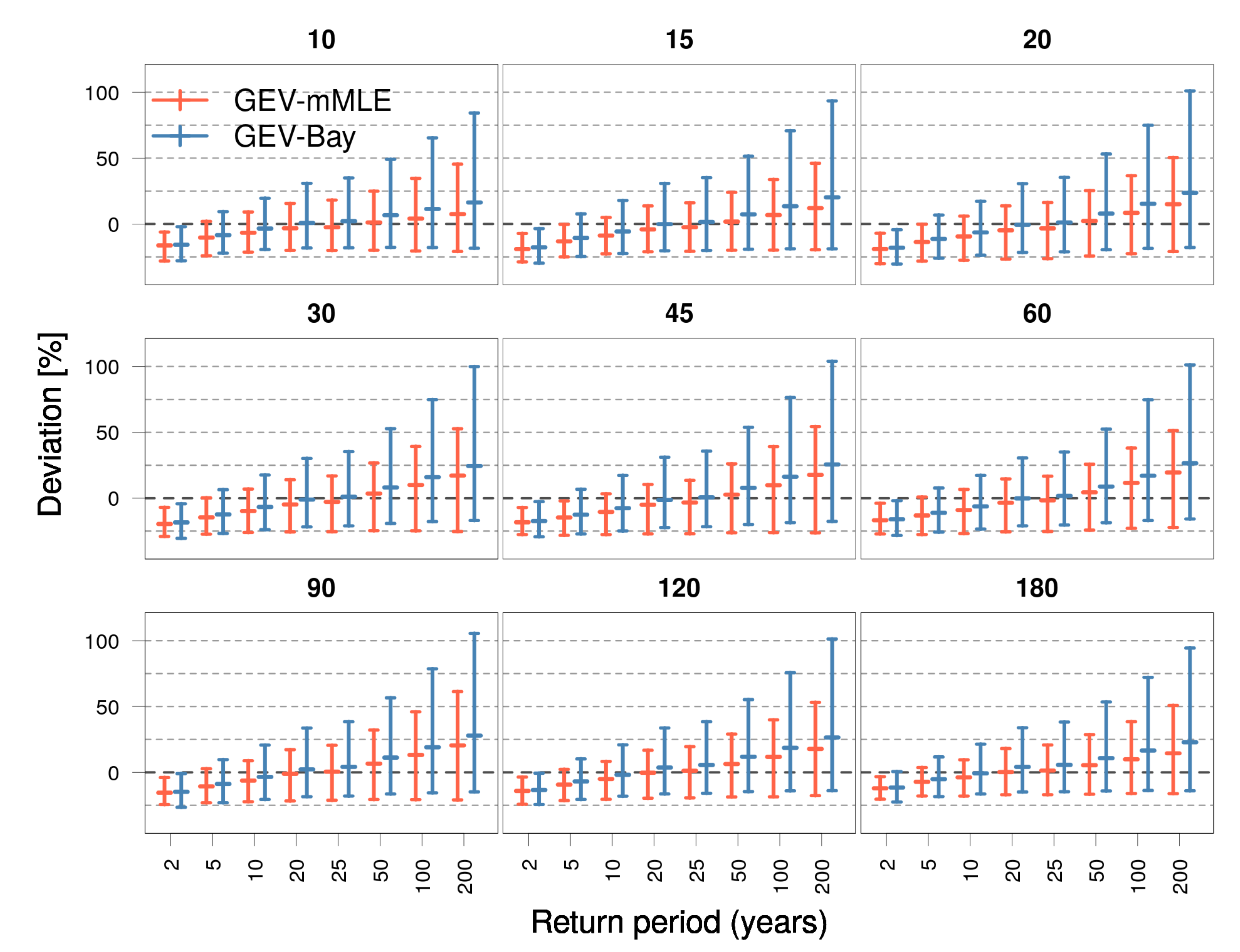
Figure 3 compares the estimated return values from the three methods for durations 10–180 min and 2- to 200-year return periods at station 18701 Oslo-Blindern. Both the GEV-mML and GEV-Bay estimates are lower than Gumbel-RV for short return periods, similar to return periods from about 20 to 50 years, and slightly higher for the longest return periods. This means that the 10- and 20-year return values that are amongst the most-used return periods (see Section 2.3) do not deviate much between the methods, while the 200-year return values increase significantly, especially with GEV-Bay.
With the exception of the 2-year return period, Gumbel-RV lies within the 95% confidence interval of GEV-mML and the 95% credible interval of GEV-Bay at Oslo-Blindern station. The confidence interval and the credible interval for longer return periods are highly different between the two GEV methods, particularly the upper limit, being much higher for GEV-Bay.
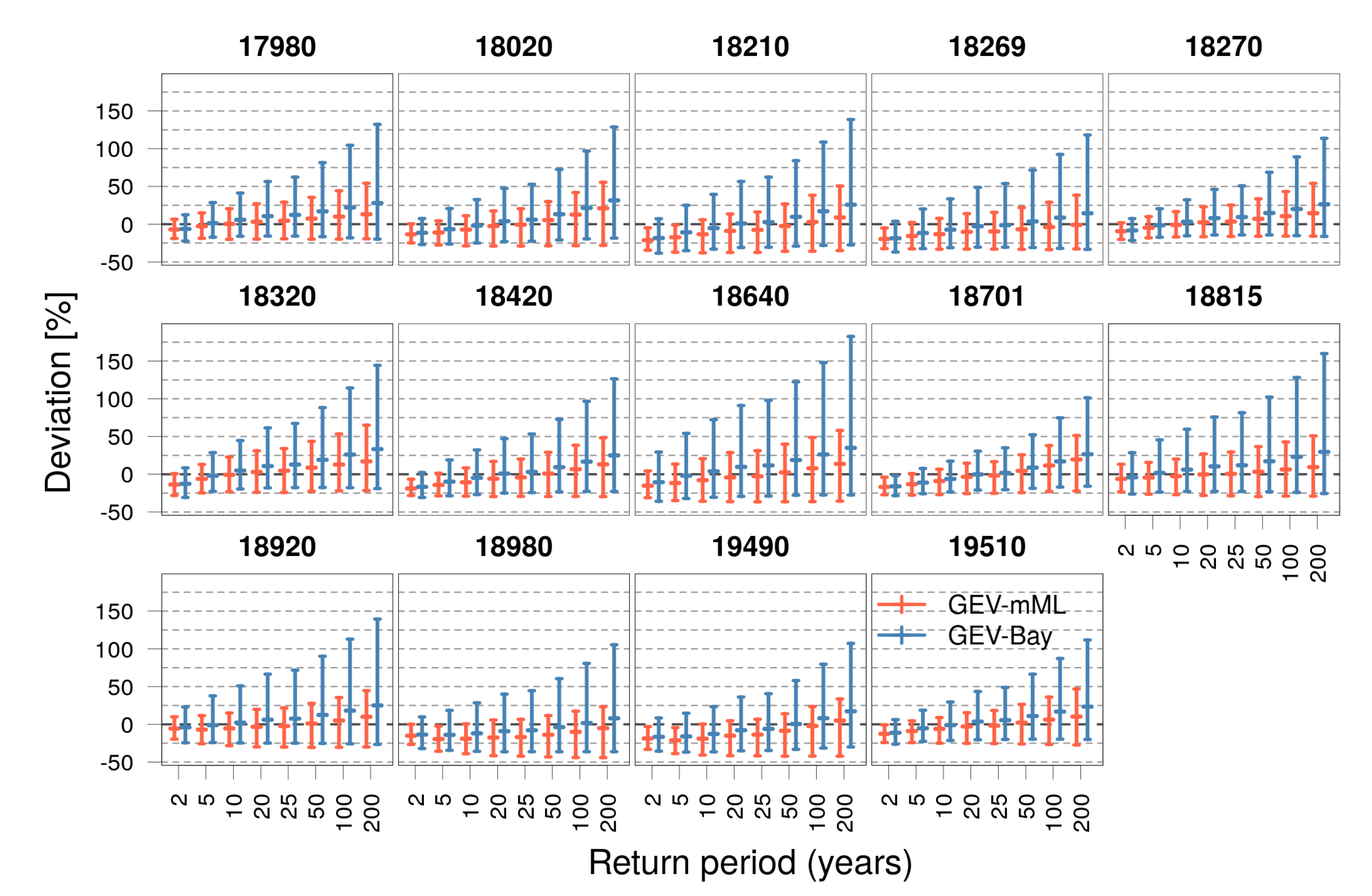
Similar results are shown in Figure 4, where we do the same comparison for all 14 stations, focusing on the 60 min duration. Note that we focus on this duration to show the difference for all stations in one figure, but the results are similar for all durations (not shown). The relatively low GEV-mML estimates are, however, even lower compared to GEV-Bay at several stations. This is particularly true for station 18980, where GEV-mML estimates are also lower than Gumbel-RV for all return periods. However, this station has only 13 years of data, which results in very uncertain IDF values. Again, the 10- and 20-year return values do not deviate much between the methods, except at station 18980, as mentioned above. The 200-year value increases with GEV-Bay at all stations, while GEV-mML only slightly overestimates at most stations compared to Gumbel-RV. Station 18640, having a short AM time series of 13 years covering the period 1974–1998, has the widest credible interval of all stations for GEV-Bay.
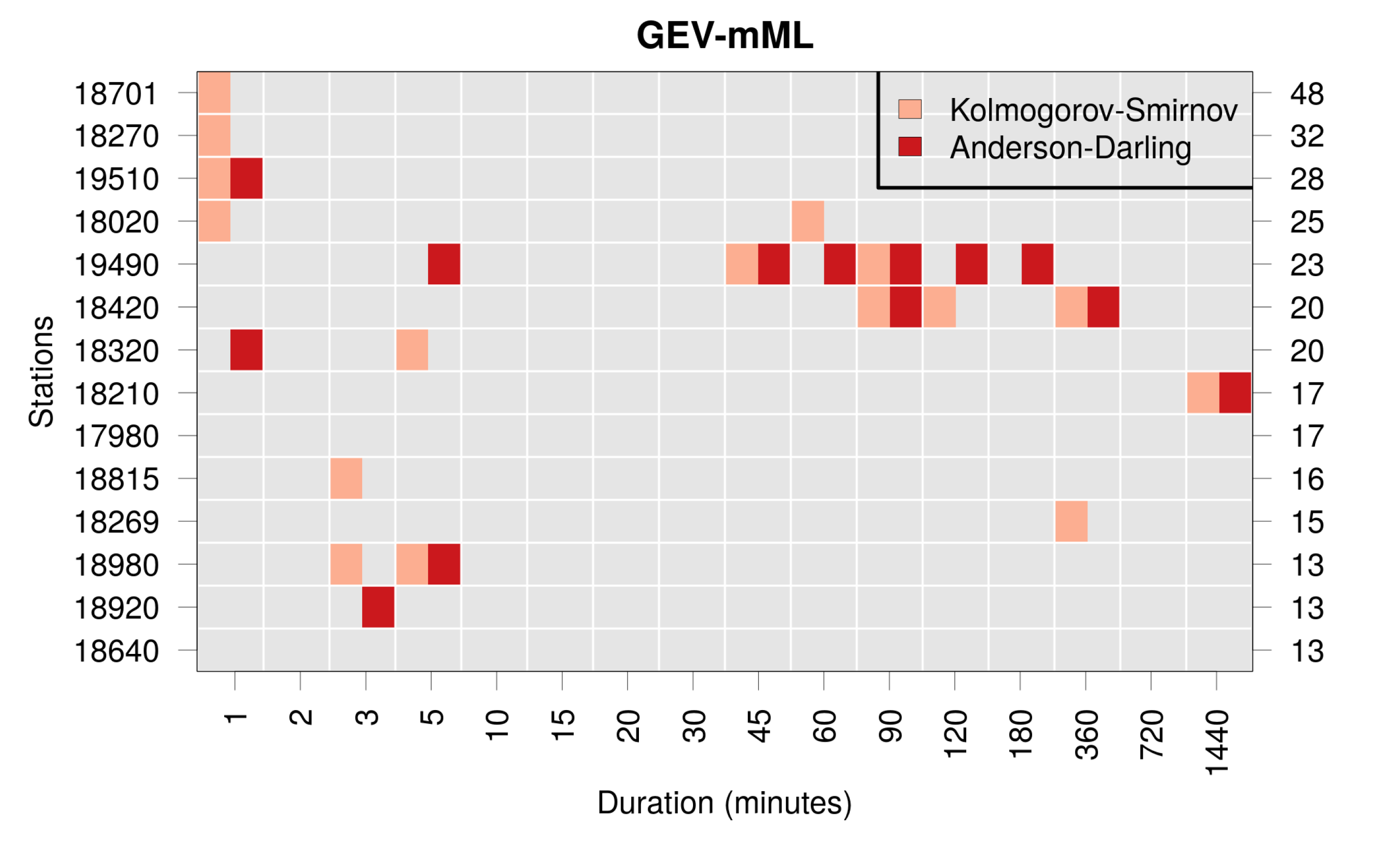
Figure 5 shows the results from the goodness-of-fit tests for GEV-mML. It can be seen that the null hypothesis ( H 0 ) is rejected several times at the 5% level. For GEV-Bay, the results are not shown as H 0 is not rejected at all at the 5% level. Note that the Kolmogorov–Smirnov test focuses on the general statistics, while the right-tailed Anderson–Darling test focuses on the longer return periods. The scores for GEV-mML indicate that the fit for station 19490 is poor: H 0 is rejected for several durations, especially for long return periods. GEV-mML features two stations (17980 and 18640) with no rejection of H 0 for any duration. On the whole, the test scores clearly favour the GEV-Bay method.

3.2. The Shape Parameter

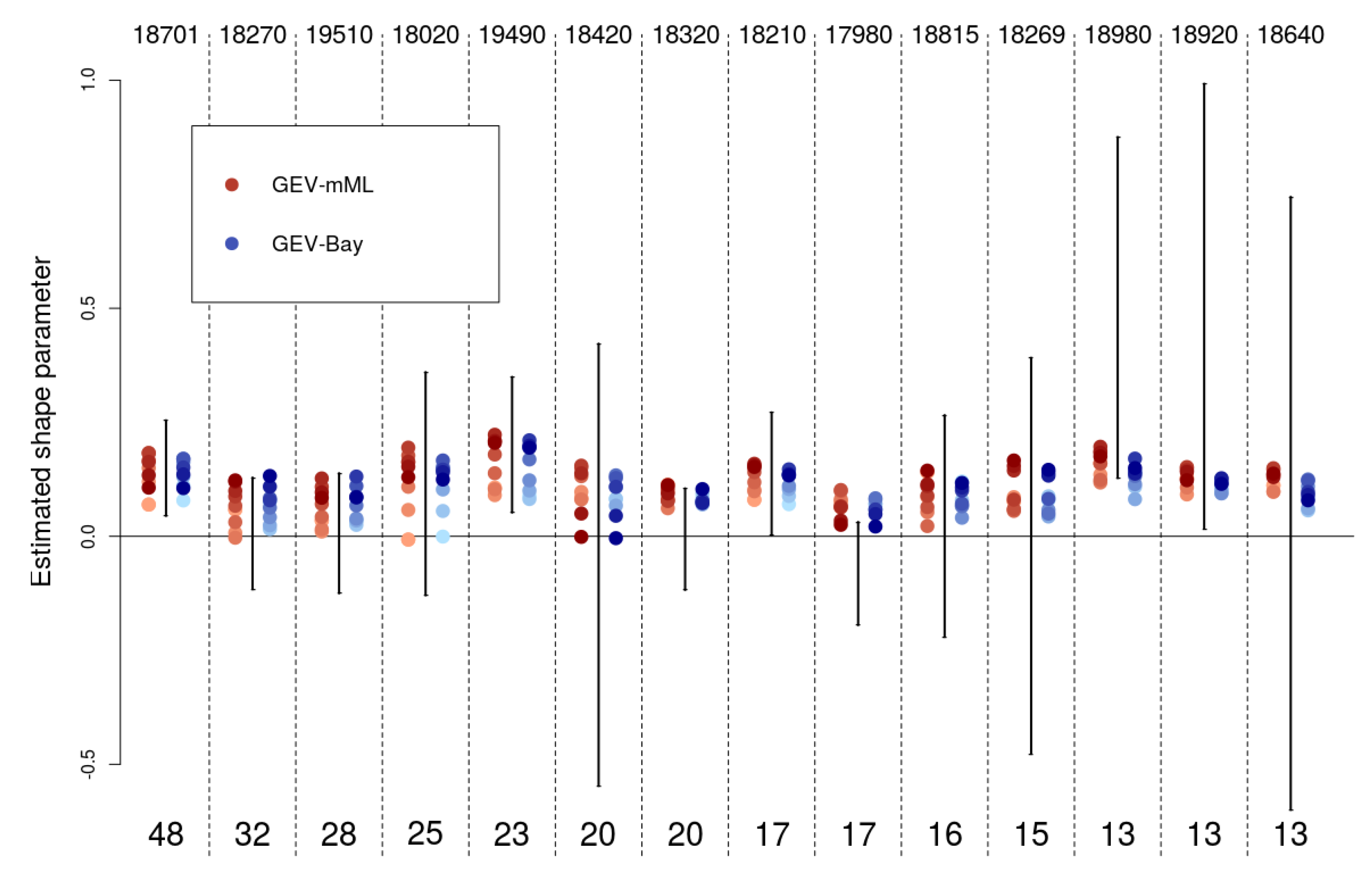
In Figure 6, we compare the shape parameter, ξ , estimated from GEV-mML, GEV-Bay, and from ordinary ML estimation, without restriction on ξ . As GEV-mML and GEV-Bay apply the same prior on ξ , their estimates are very similar. At all stations (sorted by time-series length from left to right) and all durations, ξ values are predominantly positive and vary within a narrow range. There is a slight tendency to higher values with longer durations (darker colours). Ordinary ML estimates are, on the other hand, much more variable between stations, and cover a larger range, including negative values. The largest range, that is, the most uncertain estimates with ordinary ML, is seen at station 18640. This station has a short time-series (13 years) that covers a period quite far back in time (1974–1998). Generally, stations with longer time series (>20 years) exhibit relatively small variability and are very similar to estimates from GEV-mML and GEV-Bay, indicating the effect of long time series on ξ , as shown in [5,18], for example. This also increases our confidence of the ξ estimates at, for instance, station 18701 with a time series of 48 years. Still, the lower bound of the 95% credible interval of ξ , computed with GEV-Bay, is negative for most stations and durations (not shown). Consequently, we cannot entirely rule out the possibility of Gumbel being the correct distribution, although our results show a higher likelihood for the Fréchet distribution ( ξ > 0 ) .

3.3. Assessment of Uncertainty

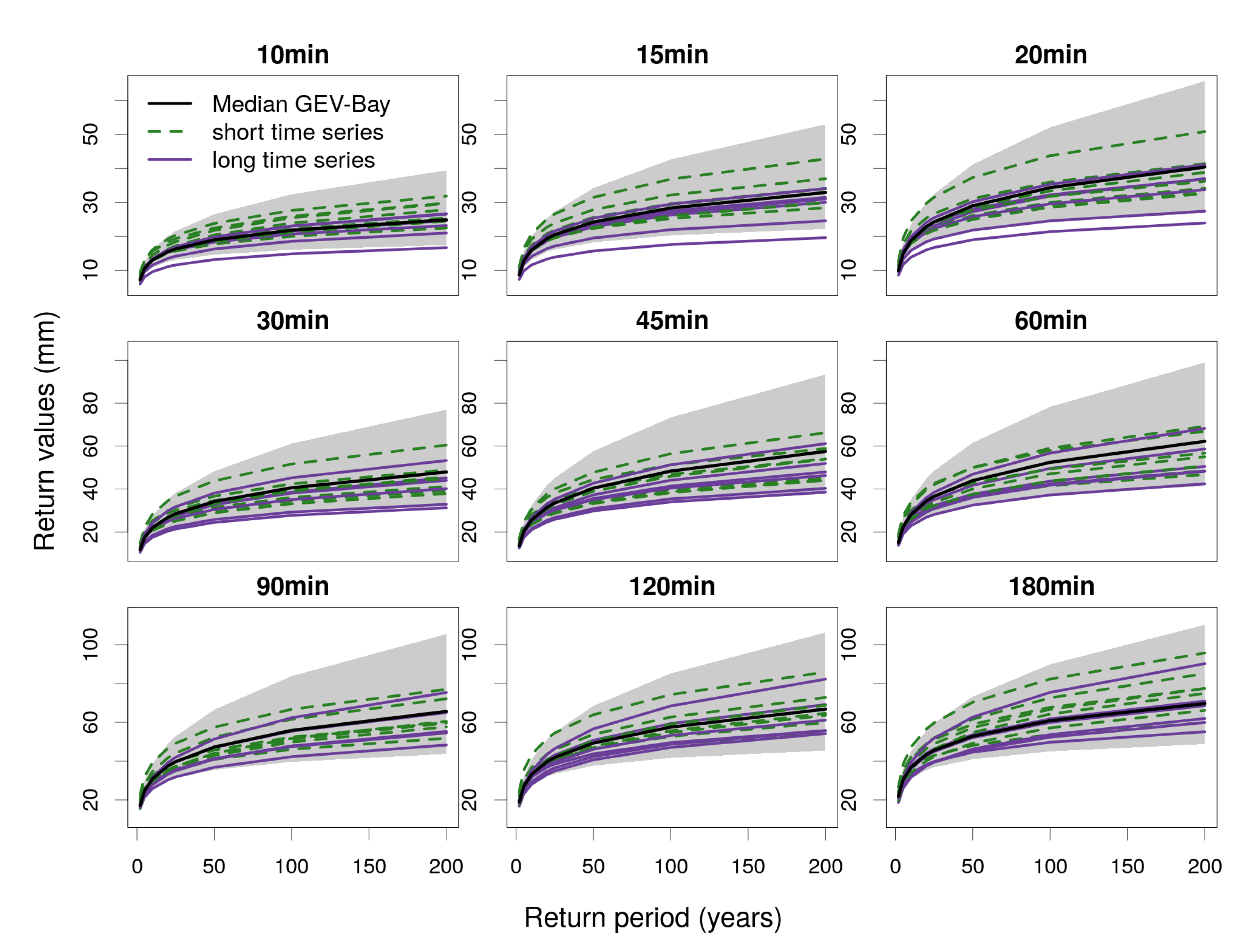
In Figure 7 and Figure 8, confidence intervals (GEV-mML and GEV-Bay, respectively) for station 18701 Oslo-Blindern are illustrated, along with median estimates of return values for all stations, divided in time series that are longer or shorter than 20 years. For both methods, we see that most stations with long time-series (>20 years) have lower estimates than Oslo-Blindern. Generally, the estimated medians at stations with short time-series are higher than at stations with longer time series. Most medians lie within the 95% confidence interval of Oslo-Blindern. Exceptions include two stations (19510 and 18270) at the shortest durations of GEV-mML, where their estimates lie below the lower confidence bound, and one station (18815) lying above the upper confidence bound at long durations and short return periods. For GEV-Bay and short-durations, station 19510 again lies below the credible interval of Oslo-Blindern.
We have also tested classifying stations according to elevation, geographical zones, or closeness to the sea, but no clear pattern was detected (not shown).

4. Discussion

Comparing GEV-mML and GEV-Bay, we see that the median estimates are quite similar, but there are partly large differences in the upper confidence bounds. As pointed out by several studies (e.g., [16,29,48]), the Bayesian framework provides a natural uncertainty assessment for model parameters and predictions, because it is presented explicitly as a posterior distribution. In contrast, the confidence intervals for GEV-mML are computed with parametric resampling, giving more narrow distributions for the shape, location, and scale parameters. These narrow distributions lead to narrow confidence intervals. In the case of the Bayesian inference on short time-series, the posterior distribution of the shape, location, and scale parameters approximates the prior distribution (for many MCMC iterations, it basically corresponds to the prior distribution). This means that the observations contain only little information that can change the prior. The resulting distributions are broader than those from GEV-mML (the prior being broad as well), resulting in broader credible intervals. Here, short time-series refer to most of the stations studied. Several tests show that only for considerably longer time periods (e.g., 100 years) the distributions for the fitting parameters from GEV-mML and GEV-Bay approximate each other, thus leading to confidence intervals that are very close (not shown).
The use of AM series instead of N-highest series leads to partially lower return values for short return periods due to generally lower precipitation amounts in the AM series. For longer return periods, the return values estimated by GEV methods are higher than values estimated by Gumbel-RV, because the positive shape parameter for the GEV distribution results in higher values. Moving from N-highest series to AM series, and from the two-parameter Gumbel ( ξ = 0 ) to the three-parameter GEV ( ξ 0 ) distribution will thus have partly large implications on the official IDF curves in Norway. This is, however, a necessary step as Gumbel-RV tends to underestimate the largest extremes. Besides, fitting Gumbel to N-highest series (as in Gumbel-RV) contradicts the theory that block maxima follow a GEV/Gumbel distribution (e.g., [17]). It is important to note that these deviances are only valid for the stations studied here, while for other parts of the country, implications may be different. Preliminary results of comparing GEV-mML and Gumbel-RV for all IDF stations in Norway (not shown here) reveal the same tendencies; generally, there are lower IDF values for short return periods (up to 50 years, approximately) and higher IDF values for long return periods, but with some exceptions in the western part of the country. In the preliminary analysis, we found slightly negative shape values at some stations in the western part, resulting in lower IDF values for long durations and long return periods compared to Gumbel-RV. These stations need special attention before the operationalising of the GEV-Bay method.
The extrapolation far beyond time-series lengths introduces large uncertainties in estimated IDF values. Uncertainty also results from other sources, namely, measurement errors, the potential mixture of extreme distributions, and the choice of distribution and method. As shown here, the choice of method for confidence interval estimation introduces additional uncertainty. The answer to how uncertainty information should be brought into the design of infrastructure can only be obtained through continuous dialogue and collaboration between us as scientists and practitioners. Probabilistic risk assessment is becoming a frequently used tool, and would be natural to introduce also in infrastructure design. Doorn and Hansson [49] found four arguments in the literature that support the use of probabilistic approaches to design over deterministic ones, such as safety factors: (1) their output can be used as an input into economic optimisation; (2) probabilistic analysis is able to provide a more precise description of the design parameters; (3) their presumed ability to provide a more integrated assessment of the safety of the full system; and (4) being more compatible with the organisational division between risk assessment and risk management. However, they also point out the one-sided focus that probabilistic risk assessment has on the elements that can be assigned probabilities, leaving out potential dangers that cannot be quantified.
Although we state in the Introduction (see Section 1) that extreme precipitation statistics in Norway are representative only for small regions, we believe that within the very small region studied here, most of the variability in IDF values is a consequence of short time-series and the high degree of coincidence associated with convective events. Nevertheless, there are rather large differences in estimated values between stations that suggest that we cannot rule out a real climatic variability. Many practitioners in Oslo use the IDF curve from station 18701 Oslo-Blindern as the default, due to its long and relatively complete time series. We have seen here that estimated confidence intervals are relatively narrow at this station, and that the ξ estimates are very similar between GEV-mML, GEV-Bay, and ordinary ML, increasing the confidence in the estimates. Goodness-of-fit tests show that the GEV-Bay estimates for Oslo-Blindern are well-fitted for the durations and return periods we have studied here. Most of the GEV-Bay median estimates for the stations in the Oslo area fall within the 95% credible interval of the 18701 Oslo-Blindern estimates for these durations and return periods.
As return values are estimated for each duration separately, inconsistencies in IDF curves may occur. Many countries use some sort of curve-fitting method to account for this (e.g., [13,50]), and obtain realistic relationships between the different durations. In a four-year project (ClimDesign) funded by the Norwegian Research council, such a curve-fitting method will be developed. In addition, methods dealing with any non-stationarity will be explored.

5. Conclusions

In this paper, we have presented an extreme value analysis of sub-daily precipitation in and close to Oslo, Norway, comparing three methods for IDF estimation. We have shown that fitting the GEV distribution to annual maximum precipitation generally gives lower estimates for short return periods and larger estimates for longer return periods compared to current methodology (Gumbel-RV). This is true for both GEV parameter estimation methods tested: (a) the modified Maximum Likelihood estimation (GEV-mML) and (b) Bayesian inference (GEV-Bay). We have also demonstrated that the GEV ξ parameter is most likely positive at all stations and for all durations, and that there is a need to restrict ξ , particularly when the time series are short. Although median estimates from GEV-mML and GEV-Bay are mostly similar, GEV-Bay outperformed GEV-mML at all stations and all durations studied. Based on these results, and given that the higher upper credible interval boundaries of GEV-Bay implies a lower risk, we recommend to proceed using GEV-Bay to estimate IDF values in Norway, and equally importantly, to provide a measure of uncertainty in terms of credible intervals. However, some important tasks remain. We need to assess how well GEV-Bay performs in other parts of Norway, and quantify the change from old to new IDF estimates. As mentioned in Section 4, a curve-fitting method is necessary to ensure consistency between durations in the individual IDF curves. We also recommend initiating dialogue with users on how to best communicate uncertainty, and how to use this information in practise.
In addition to the tasks above, there is a need for classification of IDF curves according to their quality. Criteria for classification include time-series length, a period of good-quality observations, goodness-of-fit scores, and the uncertainty in terms of credible intervals.
With its long time-series of 48 years, good GEV fit according to goodness-of-fit tests considered here, and the fact that most stations lie within the 95% confidence interval of Oslo-Blindern, we tentatively say that we find it acceptable to use estimates for this station as the default for Oslo, as long as the credible intervals are provided, understood, and considered by practitioners. However, if the median estimates for the closest station to the engineering site are higher than the median estimates for Oslo-Blindern, this must be communicated and taken into consideration.

6. Data Availability

In accordance with MET Norway’s data policy, MET Norway’s official data sources and products are freely available to the public for use, dissemination, and further processing. Measurements are available from https://frost.met.no/index.html.

Author Contributions

Conceptualization, J.L., A.V.D. and L.G.; Data curation, L.G.; Formal analysis, J.L., A.V.D. and L.G.; Funding acquisition, A.V.D. and L.G.; Investigation, J.L., A.V.D. and L.G.; Methodology, J.L., A.V.D. and L.G.; Project administration, A.V.D.; Resources, J.L., A.V.D. and L.G.; Software, J.L., A.V.D. and L.G.; Supervision, A.V.D.; Validation, J.L., A.V.D. and L.G.; Visualization, J.L., A.V.D. and L.G.; Writing—original draft, J.L., A.V.D. and L.G.; Writing—review & editing, J.L., A.V.D. and L.G. All authors have read and agreed to the published version of the manuscript.

Funding

This research was funded by the Norwegian Research council project named SURF (NFR-281022).

Acknowledgments

We thank Per-Ove Kjensli and Åse Moen Vidal at MET Norway, for their contribution to ensure data quality.

Conflicts of Interest

The authors declare no conflict of interest.

References

  1. Sorteberg, A.; Lawrence, D.; Dyrrdal, A.V.; Mayer, S.; Engeland, K. Climatic Changes in short-duration Extreme Precipitation and Rapid Onset Flooding—Implications for Design Values; Technical Report 1; Norwegian Centre for Climate Services: Oslo, Norway, 2018. [Google Scholar]
  2. Hodges, K.I.; Lee, R.W.; Bengtsson, L. A comparison of extratropical cyclones in recent reanalyses ERA-Interim, NASA MERRA, NCEP CFSR, and JRA-25. J. Clim. 2011, 24, 4888–4906. [Google Scholar] [CrossRef]
  3. Azad, R.; Sorteberg, A. Extreme daily precipitation in coastal western Norway and the link to atmospheric rivers. J. Geophys. Res. Atmos. 2017, 122, 2080–2095. [Google Scholar] [CrossRef]
  4. Dyrrdal, A.V.; Lenkoski, A.; Thorarinsdottir, T.L.; Stordal, F. Bayesian hierarchical modeling of extreme hourly precipitation in Norway. Environmetrics 2015, 26, 89–106. [Google Scholar] [CrossRef] [Green Version]
  5. Dyrrdal, A.V.; Skaugen, T.; Stordal, F.; Førland, E.J. Estimating extreme areal precipitation in Norway from a gridded dataset. Hydrol. Sci. J. 2016, 61, 483–494. [Google Scholar] [CrossRef] [Green Version]
  6. Frauenfelder, R.; Solheim, A.; Isaksen, K.; Romstad, B.; Dyrrdal, A.V.; Ekseth, K.H.; Harbitz, A.; Harbitz, C.B.; Haugen, J.E.; Hygen, O.; et al. Impacts of extreme weather events on transport infrastructure in Norway. Nat. Hazards Earth Syst. Sci. Discuss. 2017, 1–24. [Google Scholar] [CrossRef]
  7. Handmer, J.; Honda, Y.; Kundzewicz, Z.W.; Arnell, N.; Benito, G.; Hatfield, J.; Mohamed, I.F.; Peduzzi, P.; Wu, S.; Sherstyukov, B.; et al. Changes in impacts of climate extremes: Human systems and ecosystems. In Managing the Risks of Extreme Events and Disasters to Advance Climate Change Adaptation. A Special Report of Working Groups I and II of the Intergovernmental Panel on Climate Change (IPCC); Cambridge University Press: Cambridge, UK; New York, NY, USA, 2012; pp. 231–290. [Google Scholar]
  8. NOU. Overvann i byer og tettsteder—Som problem og ressurs. In English: Stormwater In Cities and Towns—As A Problem and Resource; Technical Report 16; Official Norwegian Reports; Norwegian Government Security and Service Organisation: Oslo, Norway, 2015. [Google Scholar]
  9. Li, H.; Gao, H.; Zhou, Y.; Xu, C.Y.; Ortega M., R.Z.; Sælthun, N.R. Usage of SIMWE model to model urban overland flood: A case study in Oslo. Hydrol. Res. 2020, 51, 366–380. [Google Scholar] [CrossRef]
  10. Bernard, M.M. Formulas for rainfall intensities of long duration. Trans. Am. Soc. Civ. Eng. 1932, 96, 592–606. [Google Scholar]
  11. Jenkinson, A.F. The frequency distribution of the annual maximum (or minimum) values of meteorological elements. Q. J. R. Meteorol. Soc. 1955, 81, 158–171. [Google Scholar] [CrossRef]
  12. Hosking, J.R.; Wallis, J.R. Parameter and quantile estimation for the generalized Pareto distribution. Technometrics 1987, 29, 339–349. [Google Scholar] [CrossRef]
  13. Olsson, J.; Södling, J.; Berg, P.; Wern, L.; Eronn, A. Short-duration rainfall extremes in Sweden: A regional analysis. Hydrol. Res. 2019, 50, 945–960. [Google Scholar] [CrossRef]
  14. Goudenhoofdt, E.; Delobbe, L.; Willems, P. Regional frequency analysis of extreme rainfall in Belgium based on radar estimates. Hydrol. Earth Syst. Sci. 2017, 21, 5385. [Google Scholar] [CrossRef] [Green Version]
  15. Fukutome, S.; Schindler, A.C.A. Meteoswiss Extreme Value Analyses: User Manual and Documentation, 3rd ed.; Technical Report 255; Meteo Swiss: Zurich, Switzerland, 2018; p. 80. [Google Scholar]
  16. Huard, D.; Mailhot, A.; Duchesne, S. Bayesian estimation of intensity–duration–frequency curves and of the return period associated to a given rainfall event. Stoch. Environ. Res. Risk Assess. 2010, 24, 337–347. [Google Scholar] [CrossRef]
  17. Coles, S. An Introduction to Statistical Modeling of Extreme Values; Springer: London, UK, 2001. [Google Scholar]
  18. Papalexiou, S.M.; Koutsoyiannis, D. Battle of extreme value distributions: A global survey on extreme daily rainfall. Water Resour. Res. 2013, 49, 187–201. [Google Scholar] [CrossRef]
  19. Koutsoyiannis, D. Statistics of extremes and estimation of extreme rainfall: I. Theoretical investigation/Statistiques de valeurs extrêmes et estimation de précipitations extrêmes: I. Recherche théorique. Hydrol. Sci. J. 2004, 49, 590. [Google Scholar] [CrossRef] [Green Version]
  20. Koutsoyiannis, D. Statistics of extremes and estimation of extreme rainfall: II. Empirical investigation of long rainfall records/Statistiques de valeurs extrêmes et estimation de précipitations extrêmes: II. Recherche empirique sur de longues séries de précipitations. Hydrol. Sci. J. 2004, 49, 610. [Google Scholar] [CrossRef]
  21. Ragulina, G.; Reitan, T. Generalized extreme value shape parameter and its nature for extreme precipitation using long time series and the Bayesian approach. Hydrol. Sci. J. 2017, 62, 863–879. [Google Scholar] [CrossRef]
  22. Gumbel, E.; Lieblein, J. Statistical Theory of Extreme Values and Some Practical Applications: A Series of Lectures; U.S. Government Printing Office: Washington, DC, USA, 1954; Volume 33, p. 51.
  23. Gumbel, E.J. Statistics of Extremes; Dover Publications: New York, NY, USA, 2004; Unabridged Republication of the Edition Published by Columbia University Press: New York, NY, USA, 1958. [Google Scholar]
  24. Němec, J. Engineering Hydrology; McGraw-Hill Publishing Company Limited: London, UK, 1972. [Google Scholar]
  25. Chow, V.T.; Maidment, D.R.; Mays, L.W. Applied Hydrology; McGraw-Hill Book Company: Singapore, 1988. [Google Scholar]
  26. Madsen, H.; Arnbjerg-Nielsen, K.; Mikkelsen, P.S. Update of regional intensity–duration–frequency curves in Denmark: Tendency towards increased storm intensities. Atmos. Res. 2009, 92, 343–349. [Google Scholar] [CrossRef]
  27. Fusek, M.; Hellebrand, R.; Michálek, J. Modelling precipitation extremes in the Czech Republic: Update of intensity-duration-frequency curves. Est. J. Earth Sci. 2016, 65, 234–247. [Google Scholar] [CrossRef]
  28. Prescott, P.; Walden, A. Maximum likelihood estimation of the parameters of the generalized extreme-value distribution. Biometrika 1980, 67, 723–724. [Google Scholar] [CrossRef]
  29. Van de Vyver, H. Bayesian estimation of rainfall intensity–duration–frequency relationships. J. Hydrol. 2015, 529, 1451–1463. [Google Scholar] [CrossRef]
  30. Coles, S.; Pericchi, L.R.; Sisson, S. A fully probabilistic approach to extreme rainfall modeling. J. Hydrol. 2003, 273, 35–50. [Google Scholar] [CrossRef]
  31. Hosking, J.R.M. L-Moments: Analysis and Estimation of Distributions Using Linear Combinations of Order Statistics, JR Statist. J. R. Stat. Society. Ser. B (Methodol.) 1990, 52, 105–124. [Google Scholar] [CrossRef]
  32. Martins, E.S.; Stedinger, J.R. Generalized maximum-likelihood generalized extreme-value quantile estimators for hydrologic data. Water Resour. Res. 2000, 36, 737–744. [Google Scholar] [CrossRef]
  33. Davison, A.C.; Hinkley, D.V. Bootstrap Methods and Their Application; Cambridge University Press: Cambridge, UK, 1997. [Google Scholar]
  34. Kyselỳ, J. A cautionary note on the use of nonparametric bootstrap for estimating uncertainties in extreme-value models. J. Appl. Meteorol. Climatol. 2008, 47, 3236–3251. [Google Scholar] [CrossRef]
  35. Holešovskỳ, J.; Fusek, M.; Blachut, V.; Michálek, J. Comparison of precipitation extremes estimation using parametric and nonparametric methods. Hydrol. Sci. J. 2016, 61, 2376–2386. [Google Scholar] [CrossRef]
  36. Bayes, T. LII. An essay towards solving a problem in the doctrine of chances. By the late Rev. Mr. Bayes, FRS communicated by Mr. Price, in a letter to John Canton, AMFR S. Philos. Trans. Royal Soc. Lond. 1763, 53, 370–418. [Google Scholar]
  37. Richey, M. The Evolution of Markov Chain Monte Carlo Methods. Am. Math. Mon. 2010, 117, 383–413. [Google Scholar] [CrossRef] [Green Version]
  38. Hastings, W.K. Monte Carlo sampling methods using Markov chains and their applications. Biometrika 1970, 57, 97–109. [Google Scholar] [CrossRef]
  39. R Core Team. R: A Language and Environment for Statistical Computing; R Foundation for Statistical Computing: Vienna, Austria, 2020. [Google Scholar]
  40. Frei, C.; Fukutome, S. gevXgpd: Extreme Value Analysis, R package version 1.4.2; GitHub: Zurich, Switzerland, 2014. [Google Scholar]
  41. Gilleland, E.; Katz, R.W. extRemes 2.0: An Extreme Value Analysis Package in R. J. Stat. Softw. 2016, 72, 1–39. [Google Scholar] [CrossRef] [Green Version]
  42. Luceño, A. Fitting the generalized Pareto distribution to data using maximum goodness-of-fit estimators. Comput. Stat. Data Anal. 2006, 51, 904–917. [Google Scholar] [CrossRef]
  43. Lilliefors, H.W. On the Kolmogorov–Smirnov test for normality with mean and variance unknown. J. Am. Stat. Assoc. 1967, 62, 399–402. [Google Scholar] [CrossRef]
  44. Laio, F. Cramer–von Mises and Anderson-Darling goodness of fit tests for extreme value distributions with unknown parameters. Water Resour. Res. 2004, 40. [Google Scholar] [CrossRef]
  45. Gelman, A.; Carlin, J.B.; Stern, H.S.; Dunson, D.B.; Vehtari, A.; Rubin, D.B. Bayesian Data Analysis; CRC Press: Boca Raton, FL, USA, 2013. [Google Scholar]
  46. Berkhof, J.; Van Mechelen, I.; Hoijtink, H. Posterior predictive checks: Principles and discussion. Comput. Stat. 2000, 15, 337–354. [Google Scholar] [CrossRef]
  47. Van de Schoot, R.; Kaplan, D.; Denissen, J.; Asendorpf, J.B.; Neyer, F.J.; Van Aken, M.A. A gentle introduction to Bayesian analysis: Applications to developmental research. Child Dev. 2014, 85, 842–860. [Google Scholar] [CrossRef]
  48. Reich, B.J.; Shaby, B.A. A hierarchical max-stable spatial model for extreme precipitation. Ann. Appl. Stat. 2012, 6, 1430. [Google Scholar] [CrossRef]
  49. Doorn, N.; Hansson, S.O. Should probabilistic design replace safety factors? Philos. Technol. 2011, 24, 151–168. [Google Scholar] [CrossRef] [Green Version]
  50. Di Baldassarre, G.; Brath, A.; Montanari, A. Reliability of different depth-duration-frequency equations for estimating short-duration design storms. Water Resour. Res. 2006, 42, 151–168. [Google Scholar] [CrossRef]
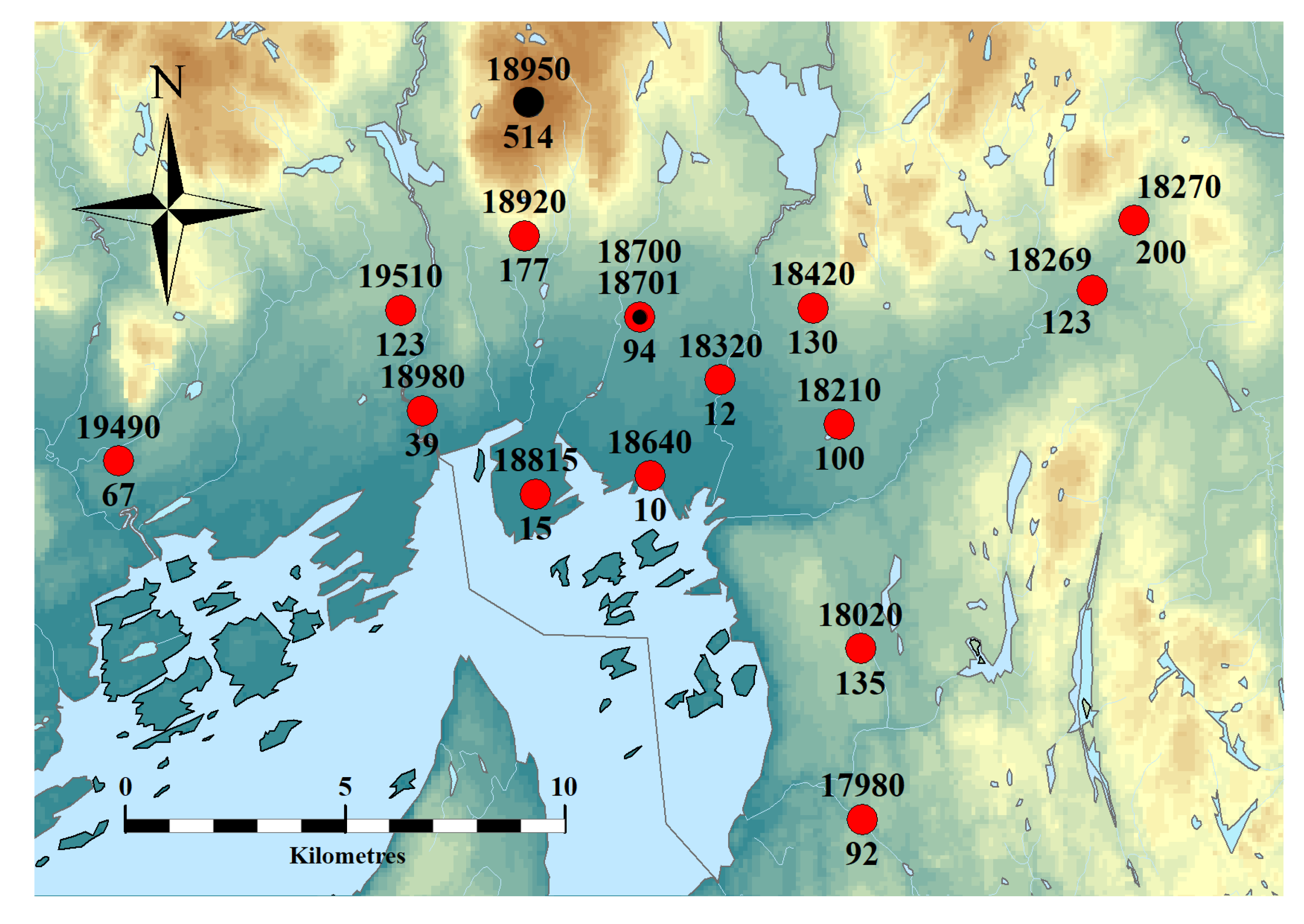
Figure 1. Map of tipping bucket pluviometer stations (red dots) in the general Oslo area. Numbers above the dots indicate the station ID, and numbers below the dots indicate the height above sea level in meters. Black dots (18700 and 18950) show weight gauges used for analysing monthly maximum precipitation (see Section 2.1.2). The reference pluviometer at MET Norway is 18701 Oslo-Blindern.
Water 12 01735 g001
Figure 2. Annual maximum of 1, 2, and 3 h precipitation by month at the stations 18700 Oslo-Blindern and 18950 Tryvannshøgda. See Figure 1 for station location.
Water 12 01735 g002
Figure 3. Relative difference to return levels from Gumbel-RV for GEV-mML (red) and GEV-Bay (blue) at station 18701 Oslo-Blindern for the durations of 10–180 min and all return periods. The bars indicate the 95% confidence or credible interval.
Water 12 01735 g003
Figure 4. Relative difference to return levels from Gumbel-RV for GEV-mML (red) and GEV-Bay (blue) for all stations and all return periods. Only the 60 min precipitation is shown. The bars indicate the 95% confidence or credible interval.
Water 12 01735 g004
Figure 5. Test scores for GEV-mML for all stations (y-axis) and all durations (x-axis). The reddish colours indicate stations and durations where the null hypothesis H 0 is rejected at α = 5 % . H 0 states that the empirical and estimated distribution are the same. Stations are sorted by time-series length (indicated on the right) from bottom to top.
Water 12 01735 g005
Figure 6. The GEV shape parameter estimated with GEV-mML (red) and GEV-Bay (blue) for all durations (vertically) and stations (horizontally). The black lines show the minimum and the maximum shape parameter estimated by ordinary ML. The different shades indicate the duration, from light (short-duration) to dark (long duration). Stations are sorted by time-series length (number on the bottom) from left to right. Station numbers are indicated on the top.
Water 12 01735 g006
Figure 7. Confidence interval (grey) and median (black) of return values for Oslo-Blindern station (18701), estimated with GEV-mML. Median values for the other stations are shown as green dashed lines if the observed time series is shorter than 20 years, and as purple solid lines if observations are longer than 20 years.
Water 12 01735 g007
Figure 8. As in Figure 7, but for GEV-Bay.
Water 12 01735 g008
Table 1. Station IDs, station names, and the time period in operation. N-highest: N-highest measurements for each duration, N being the number of years; AM: annual maxima for each duration.
IDStation NameOperational PeriodNumber of Seasons
FromToN-HighestAM
17980Oslo-Ljabruveien1 January 2000-2017
18020Oslo-Lambertseter15 May 1985-3525
18210Oslo-Hovin15 January 1999-2017
18269Oslo-Haugenstua1 January 2000-1615
18270Oslo-Vestli18 April 1974-3732
18320Oslo-Hausmannsgate21 June 19844 November 20132920
18420Oslo-Disen2 June 1998-2120
18640Oslo-Vestre Vika22 May 19743 October 19981513
18701Oslo-Blindern plu16 April 1968-5248
18815Oslo-Bygdøy1 January 2000-1816
18920Oslo-Besserud29 September 1998-1713
18980Oslo-Lilleaker1 January 2000-1413
19490Gjettum1 July 1970-3423
19510Øvrevoll19 May 1967-3828
Table 2. Goodness-of-fit test scores used in this study and their computational form. Note that z i = F ( x i ) , where F ( x ) is the theoretical cumulative distribution function and x = { x 1 , , x n } is the observed sample.
Test ScoreComputational Form
Kolmogorov–Smirnov statistic 1 2 n + max 1 i n | z i i 1 / 2 n |
Right-tail Anderson–Darling statistic n 2 2 i = 1 n z i 1 n i = 1 n ( 2 i 1 ) ln ( 1 z n + 1 i )