Evaluating Maize Drought and Wet Stress in a Converted Japanese Paddy Field Using a SWAP Model

Abstract

Japanese government recommend farmers to cultivate upland crops in paddy fields (“converted fields”) to suppress the overproduction of rice. Converted fields are subject to excessively wet and dry conditions that reduce the yield of non-rice crops. Drought and wet stresses are critical to crop growth within specific growth periods. To provide data for use in mitigating crop yield reduction, we evaluated drought and wet stresses in maize (Zea mays L.). A SWAP (soil–water–atmosphere–plant) model was applied to a converted maize field. Observations were carried out in 2019 and 2018 for model calibration and validation. Thereafter, we evaluated the water stress of maize in 2019 (actual conditions) and at a tillage depth 11 cm deeper (scenario conditions). We found that (1) drought and wet stresses occurred within the relevant critical growth periods under actual conditions; (2) in the critical periods, the drought and wet stresses under scenario conditions were 33%–75% and 10%–82%, respectively, of those under actual conditions; (3) water stress at depths of 10 and 20 cm was lower under the scenario conditions than under the actual conditions. These results indicate that deeper tillage may mitigate both drought and wet stresses and can be used to reduce water stress damage in converted fields.

1. Introduction

In order to regulate rice production in relation to demand for it and other agricultural products, maize and other “upland” crops are cultivated in temporarily drained paddy fields, known as “converted fields”, in Japan [1]. The drainage in paddy fields is poor, mainly due to hardpans that exist at approximately 20 cm below the soil surface. Converted fields are therefore at risk of waterlogging. Moreover, we must consider the interaction of weather conditions during the cultivation period. This period in Japan often includes the rainy season (from mid-June to mid-July, after mid-September), the dry season (from mid-July to beginning of September). Therefore, both drought and wet stresses often reduce upland crop yields, including those from converted fields [2].

Maize (Zea mays L.) cultivation for feed has been attempted in converted fields in southwestern Japan. Previous studies have shown that drought and wet stresses must be considered in relation to specific growth periods for maize cultivation. Çakir [3] demonstrated that drought stress at the beginning of the vegetative or tasselling growth stages reduced crop height; irrigation conducted approximately 40–65 days after emergence of maize could eliminate this effect (tasselling is the stage at which stamens appear, following maximum growth). Moreover, Kanwar et al. [4] showed that maize yield was most significantly affected by wet stress at the flowering stage: 60–80 days after planting.

To quantify drought and wet stresses on the crop separately, we used a SWAP (soil–water–atmosphere–plant) model [5,6] in this study. This model quantifies those stresses using crops’ critical pressure heads and has been applied in several studies. Anan et al. [7] evaluated the stresses in potato plants from precipitation and continuous drought in a reclaimed crop field, and Yuge et al. [8] conducted a scenario analysis to suggest an optimal irrigation regime in a reclaimed field with sorghum and potato. We hypothesized that we would be able to develop strategies to reduce water-related stress damage to crops by applying the SWAP model. This study focused on a converted maize field to evaluate (1) the water stress under actual field conditions and (2) the effect of tillage depth on water stress—we assumed this is one of the stress reduction strategies. We mainly evaluated draught and wet stresses in their critical growth periods [3,4].

2. Materials and Methods

2.1. SWAP Model Description

2.1.1. Soil Water Movement

A SWAP model is a vertical one-dimensional model which uses Richards’ equation to describe soil water movement:

$$\frac{\partial \theta }{\partial t}=\frac{\partial \left[K\left(h\right)\left(\frac{\partial h}{\partial z}+1\right)\right]}{\partial z}-S_a\left(z,h\right),$$

(1)

where θ is the volumetric water content (cm³ cm⁻³), t is time (d), K(h) is the unsaturated hydraulic conductivity (cm d⁻¹), h is the matric potential head (−cm), z is the vertical coordinate (cm), and S_a(z,h) is the soil water extraction rate by plant roots (cm³ cm⁻³ d⁻¹). The SWAP model can function with a time-step varying from 10⁻⁶ to 0.2 days to obtain calculation convergence.

To describe unsaturated hydraulic conductivity K(h), the SWAP model uses the Mualem–van Genuchten model [9,10]. The analytical θ(h) is described by the following equation:

$$\theta \left(h\right)={\theta }_{res}+\left({\theta }_{sat}-{\theta }_{res}\right){\left(1+{\left|\alpha h\right|}^n\right)}^{-m},$$

(2)

where θ_sat is the saturated water content (cm³ cm⁻³), θ_res is the residual water content (cm³ cm⁻³), α (cm⁻¹), n, and m (−) are empirical shape factors; and m is 1−1/n. K(h) is calculated using the following equations:

$$K\left(h\right)=K_{sat}{S}_e^{\lambda }{\left[1-{\left(1-S_e^{\frac{1}{m}}\right)}^m\right]}^2,$$

(3)

$$S_e=\frac{\theta \left(h\right)-{\theta }_{res}}{{\theta }_{sat}-{\theta }_{res}},$$

(4)

where K_sat is the saturated hydraulic conductivity (cm d⁻¹) and λ is a shape parameter (=0.5).

2.1.2. Boundary Conditions

The Penman–Monteith direct method was applied as a top boundary [11,12]:

$$T_p=\frac{\left(1-W_{frac}\right)\left(V_c\frac{{\Delta }_v}{L_w}\left(R_n-G\right)+\frac{p_1{\rho }_a{C}_a}{L_w}\left(\frac{e_{sat}-e_a}{r_{a, can}}\right)\right)}{{\Delta }_v+{\gamma }_a\left(1+\frac{r_{s, min}}{r_{a, can}LA{I}_{eff}}\right)},$$

(5)

$$E_p=\frac{\left(1-V_c\right)\frac{{\Delta }_v}{L_w}\left(R_n-G\right)+\frac{p_1{\rho }_a{C}_a}{L_w}\left(\frac{e_{sat}-e_a}{r_{a, soil}}\right)}{{\Delta }_v+{\gamma }_a\left(1+\frac{r_{soil}}{r_{a, soil}}\right)},$$

(6)

where T_p is the potential transpiration of a dry canopy (mm d⁻¹), W_frac is the fraction of the day in which the canopy is wet (−), V_c is the vegetation cover (−), ∆_v is the slope of the vapor pressure curve (kPa C⁻¹), L_w is the latent heat of vaporization (J kg⁻¹), R_n is the net radiation flux at the canopy surface (J m⁻² d⁻¹), G is the soil heat flux (J m⁻² d⁻¹), p₁ accounts for unit conversion (=86,400 s d⁻¹), ρ_a is the air density (kg m⁻³), C_a is the heat capacity of moist air (J kg⁻¹ C⁻¹), e_sat is the saturation vapor pressure (kPa), e_a is the actual vapor pressure (kPa), r_a,can is the aerodynamic resistance of the crop (s m⁻¹), γ_a is the psychrometric constant (kPa C⁻¹), r_s,min is the minimal stomatal resistance (s m⁻¹), LAI_eff is the effective leaf area index (−), E_p is the potential evaporation (mm d⁻¹), r_soil is the soil resistance of wet soil (s m⁻¹), and r_a,soil is the aerodynamic resistance of the soil surface (s m⁻¹). On a daily basis, the soil heat flux G is assumed to be negligible. The vegetation cover V_c is obtained by the following equation:

$$V_c=1-e^{-{\kappa }_{dir}{\kappa }_{dif}LAI},$$

(7)

where κ_dir and κ_dif are the extinction coefficients for direct (0.80) and diffuse (0.72) solar light, respectively, and LAI is the actual leaf area index (−). LAI_eff is derived from LAI:

$$LA{I}_{eff}=\frac{LAI}{0.3LAI+1.2},$$

(8)

The aerodynamic resistance of the crop r_a,can is determined using the resistance for uniform crop r_a,can,0:

$$r_{a, can}=\frac{r_{a, can,0}}{V_c},$$

(9)

$$r_{a,can,0}=\frac{\ln \left(\frac{z_m-d}{z_{om}}\right)·\ln \left(\frac{z_h-d}{z_{oh}}\right)}{{\kappa }_{vk}^2·u},$$

(10)

where z_m is the height of wind speed measurements (m), z_h is the height of temperature and humidity measurements (m), d is the zero plane displacement of wind profile (m), z_om is the roughness parameter for momentum (m), z_oh is the roughness parameter for heat and vapor (m), κ_vk is the von Karman constant (0.41), and u is the wind speed measurement at z_m (m s⁻¹). The parameters d, z_om, and z_oh are defined as:

$$d=\frac{2}{3}{h}_{crop},$$

(11)

$$z_{om}=0.123h_{crop},$$

(12)

$$z_{oh}=0.1z_{om}$$

(13)

where h_crop is the crop height (cm).

The SWAP model has several options for its bottom boundary condition, such as a prescribed groundwater level, a prescribed bottom flux, a bottom flux of zero, or a free drainage of soil profile. In this study, we decided to use a prescribed groundwater level, because relatively high groundwater levels were present during the field observations.

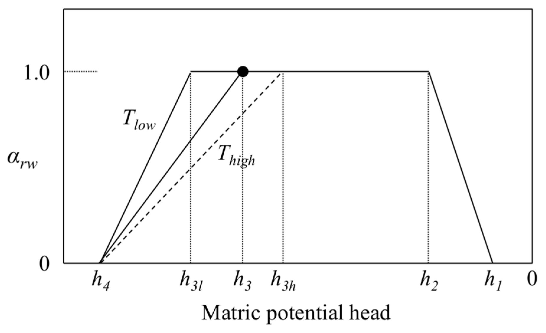
2.1.3. Crop Water Stress

The maximum possible root water extraction rate per day at a certain depth S_p(z) is calculated by the following equation using the potential transpiration T_p (cm d⁻¹):

$$S_p\left(z\right)=\frac{l_{root}\left(z\right)}{{{\displaystyle \int }}_{-D_{root}}^0{l}_{root}\left(z\right)dz}{T}_p,$$

(14)

where l_root(z) is the root length density at a certain depth (cm cm⁻³) and D_root is the root layer thickness (cm).

The root water extraction rate is reduced due to suboptimal soil conditions, namely excessively wet and dry conditions; the soil water extraction rate by plant roots S_a(z,h) is calculated considering the water stress described by the function proposed by Feddes et al. [13]:

$$S_a\left(z,h\right)={\alpha }_{rw}{S}_p\left(z\right),$$

(15)

where α_rw is the reduction factor for excessive wet and dry conditions (−). The reduction factor α_rw changes from 0 to 1.0 depending on the critical pressure heads h₁, h₂, h₃, and h₄ (Figure 1). Root water extraction is optimal between h₂ and h₃; the reduction under wet conditions occurs when wetter than h₂; under dry conditions, the reduction occurs when drier than h₃. The value of h₃ depends on the water demand of the atmosphere and varies with T_p; it is expressed by following equations:

$$h_3=h_{3l},\mathrm{for}{T}_p\le T_{low}$$

(16)

$$h_3=h_{3h}+\frac{T_{high}-T_p}{T_{high}-T_{low}}\left(h_{3l}-h_{3h}\right),\mathrm{for}{T}_{low}<T_p<T_{high}$$

(17)

$$h_3=h_{3h},\mathrm{for}{T}_p>T_{high}$$

(18)

where h_3l and h_3h are the critical pressure heads for low and high transpiration rates, T_low and T_high, respectively (−cm). We used the default values for T_low and T_high: 0.1 and 0.5 cm d⁻¹.

The actual transpiration rate T_a (cm d⁻¹) is yielded by integrating S_a(z,h) over the root layer. Drought and wet stresses are evaluated by subtracting T_a from T_p.

2.2. Field Experiment

Field observations were conducted in 2018 and 2019 at a converted field (100 × 43 m) in Okayama, Japan (37°34′53.4″ N; 113°54′11.8″ E). The soil in the field was lowland paddy soil according to the Japan soil inventory, NARO (http://soil-inventory.dc.affrc.go.jp/) [14]. The field was divided into two plots for other research purposes; for our purposes, we defined these as calibration and validation plots (Figure 2 and Figure 3). Rotary tillage was carried out to a depth of 12 cm in both plots before sowing maize for whole crop silage.

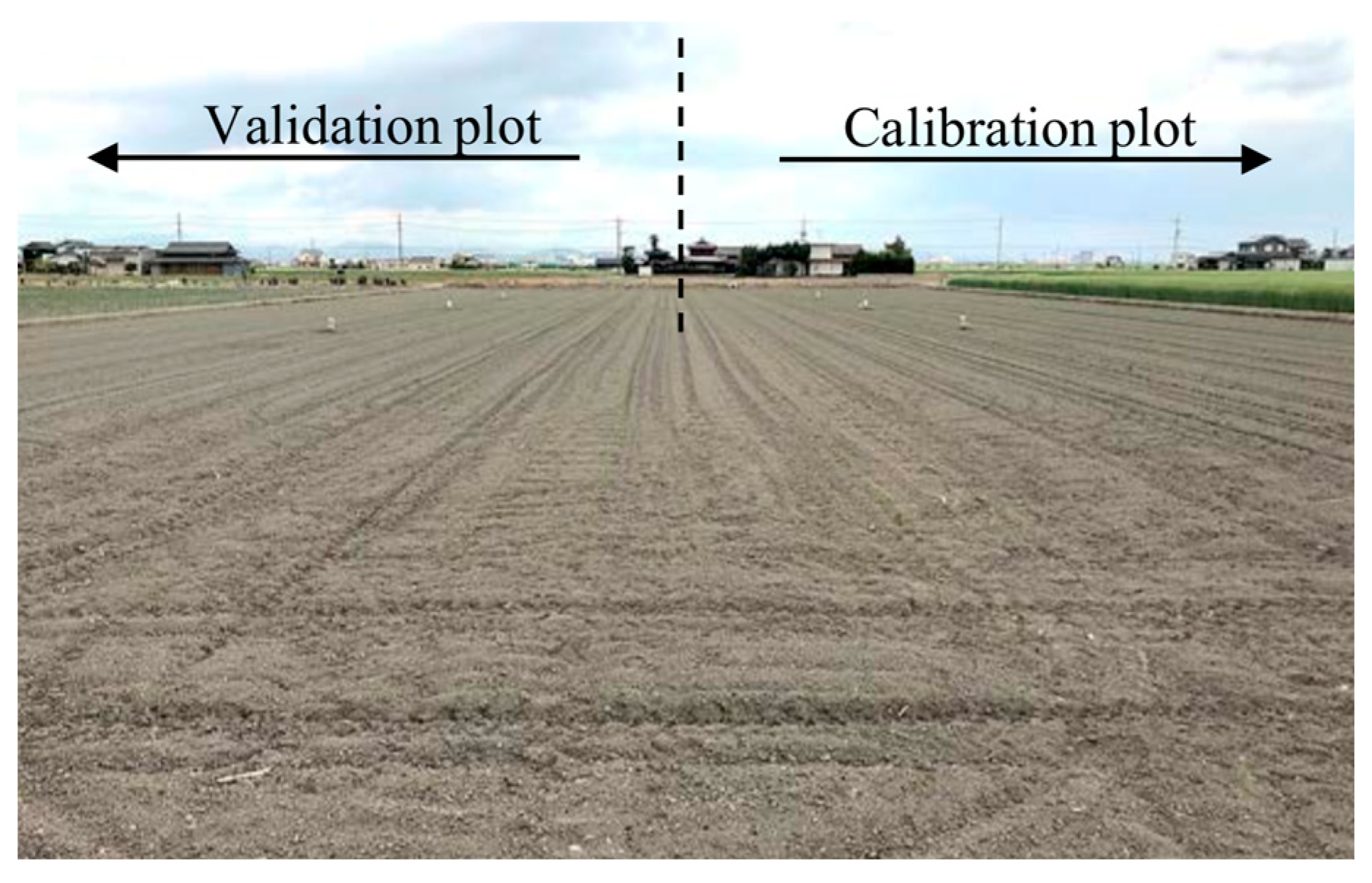
2.2.1. Field Experiment for Model Calibration

Field data for model calibration were collected in the calibration plot during the 2019 maize growing season. Maize was sown on 10 April 2019, and observations were made between 24 April and 17 July 2019. Groundwater level, as the bottom boundary, was recorded by a water level monitoring sensor (HYDROS 21; METER Group, Pullman, WA, USA) in the center of the field (Figure 3). We could not measure matric potential in our environment (i.e., low budget, labor deficit for sensor maintenance); we measured volumetric water content using capacitive soil moisture sensors (EC-5; METER Group) because they measure value accurately and are inexpensive. The sensors were set up in three locations at depths of 10, 20, and 30 cm (Figure 3). The daily change in volumetric water content for calibration was acquired by averaging the readings of the three soil moisture sensors at each depth. Volumetric water content and groundwater level were recorded every 30 min.

Prior to the field observations, we collected soil samples from depths of 10, 20, and 30 cm in the center of the field using 100 mL soil samplers (DIK-1801; Daiki Rika Kogyo Co., Kounosu, Japan) to obtain soil hydraulic data for the Mualem–van Genuchten model. Three samples were collected from each depth. Saturated hydraulic conductivity was measured by the falling head method [15]. The soil water retention curve was generated by the soil column (matric potential head range: −1 to −31.6 cm) [16] and pressure plate methods (matric potential head range: −100 to −16,000 cm) [17]. The soil hydraulic properties at each depth were determined by averaging the values obtained from the three samples.

The maize crop height was measured on 9 May, 23 May, 12 June, 25 June, and 25 July 2019. Crop height on each occasion was determined by averaging the values obtained from 10 samples. Rooting depth was measured on 17 July 2019, from a single sample, to avoid field destruction.

2.2.2. Field Experiment for Model Validation

Field data for model validation were collected in the validation plot during the 2018 maize growing season. In this plot, maize was sown on 2 August 2018, and observations were made between 10 August and 20 November 2018. Sensor installation and use were as for 2019, except that the soil moisture sensors were used only at a depth of 10 cm (Figure 3). The crop height was measured on 14 August and 5 November 2018. The rooting depth was not obtained during these observations.

2.3. Model Calibration and Validation

2.3.1. Data for SWAP Model Simulation

The SWAP model requires various input parameters to conduct a simulation, as specified in Section 2.1 above.

Table 1. Input and calibration data.

Soil hydraulic data
		Estimated by nonlinear optimization using the Mualem–van Genuchten model
	Saturated hydraulic conductivity Ksat	Measured
	Soil water retention curve	Measured
Meteorological data
		Obtained from the Agro-Meteorological Grid Square Data, NARO, which generates the Japanese meteorological data for every 1 km2 [18]
Crop data
	Crop height	Measured
	Rooting depth	Measured
	LAI	Determined based on Maddonni and Otegui [19]
	Critical pressure heads of water stress	Data from Wesseling et al. [20]
Initial and bottom boundary conditions
	Matric potential head	Converted from observed volumetric water content
	Groundwater level	Measured
Data for calibration
	Volumetric water content	Measured

shows the sources used for these data.

2.3.2. Model Calibration

The simulation period was 24 April to 17 July 2019; this is the same as the observation period for volumetric water content and groundwater level. The simulation domain was set at a depth of 100 cm. The domain was divided into three parts (layers 1, 2, and 3), based on soil sampling and soil moisture sensor depths. Initial Mualem–van Genuchten parameters from field observation were assigned to each layer. The nodal spacing increased from 0.2 cm near the soil surface to 5.0 cm with depth (

Table 2. Nodal spacing in the simulation domain.

Depth (cm)	0–3	3–23	23–35	35–100
Nodal spacing (cm)	0.2	1.0	2.0	5.0

). The initial matric potential head was obtained by transforming the initial volumetric water content, and was applied accounting for depth; below a depth of 30 cm, the lowest measurement depth, the initial matric potential head was determined based on the initial groundwater level.

Table 3. Crop data used in the simulation.

Maximum rooting depth (cm)	50.0	(17 July 2019; observed)
Crop height in the calibration plot (cm)	27.2	(9 May 2019; observed)
	58.0	(23 May 2019; observed)
	158.5	(12 June 2019; observed)
	230.1	(25 June 2019; observed)
	258.6	(17 July 2019; interpolated)
Crop height in the validation plot (cm)	17.7	(10 August 2018; observed)
	246.1	(5 November 2018; observed)
Critical pressure heads: h1, h2, h3h, h3l, h4 (−cm)	15, 30, 325, 600, 8000

Notes: Crop height was obtained by averaging the values from 10 samples. The crop height on 17 July 2019 was interpolated using data from 25 June and 25 July 2019. Critical pressure heads followed Wesseling et al. [20].

shows the crop data used in the simulation. We assumed that crop height and rooting depth were zero at the beginning of the simulation because the observed initial maize height was negligible. The rooting depth was assumed to reach its maximum depth by the end of simulation, and to increase linearly [8]. The rate of increase in crop height was based on observed values; the maximum crop height at the end of the simulation was interpolated using the observed crop heights on 25 June and 25 July 2019. We applied the default critical pressure heads for maize from Wesseling et al. [20] because it is difficult to measure. A trial and error process [21,22,23] was used to optimize soil hydraulic parameters.

2.3.3. Model Validation

Model validation was performed using the optimized soil hydraulic parameters from the calibration and observation data from 2018. The simulation period was from 10 August to 20 November 2018, to match the observation period. Calibration values were used for soil layer assignment and nodal spacing. We assumed the same maximum rooting depth, 50 cm, as for the calibration plot (Table 3). Linear interpolation, from 0 cm on the sowing date of 2 August 2018 to the maximum model depth at the end of the simulation, provided the estimate of initial rooting depth on 10 August 2018. We assumed a sowing-date crop height of 0 cm, changing in accordance with the measured height (Table 3); the initial crop height was estimated using this minimum value and the observed height on 14 August 2018. After 5 November 2018, we assumed that the height did not increase.

2.3.4. Evaluation of Calculation Error

During calibration and validation, we evaluated the agreement at each time point between the observed (θ_obs) and calculated (θ_cal) volumetric water content using the root mean square error (RMSE):

$$\mathrm{RMSE}=\sqrt{\frac{1}{N}{{\displaystyle \sum }}_{t=1}^N{\left(obs,t-cal,t\right)}^2},$$

(19)

where N is the number of time points, and obs,t and cal,t are the observed and calculated data at each time point. Moreover, we calculated RMSE between the observed and calculated matric potential head (h_obs and h_cal) in the calibration plot to consider possible error in water stress estimation; the matric potential head was converted from θ_obs and θ_cal by using calibrated Mualem–van Genuchten parameters.

2.3.5. Evaluation of Water Stress under Actual and Scenario Conditions

We estimated the daily changes in T_p, T_a, drought stress, and wet stress using the 2019 observations as the actual conditions. We then evaluated the difference in water stress between the actual and a scenario in which tillage reached 11 cm deeper than under actual conditions; the soil hydraulic properties of layer 2 were therefore the same as those of layer 1. The tillage depth in the scenario conditions assumed to exceed a depth where hardpans usually exist.

3. Results and Discussion

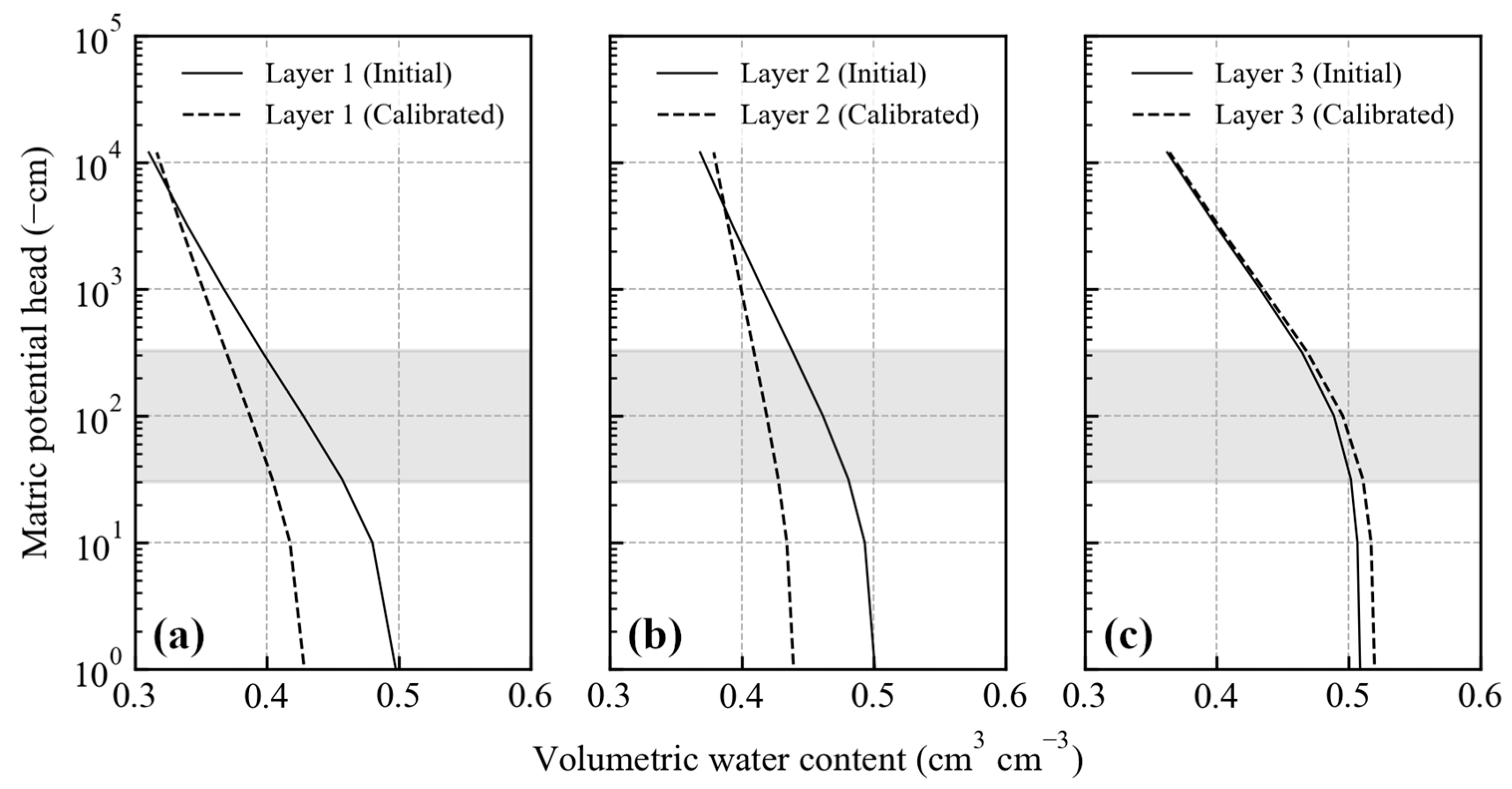
3.1. Model Calibration

During 2019, climatic conditions were typical: the weather became drier after sowing, followed by the rainy season (Figure 4a). During the study period, precipitation was highest, at 51.7 mm d⁻¹, on 15 June 2019. Thereafter, precipitation occurred more frequently. The highest groundwater level, −14.6 cm, was recorded on 2 May 2019, after which it gradually decreased to its lowest value, approximately −85 cm; we note that this was the limit of observation for the water level monitoring sensor. The groundwater level changed frequently after 15 June 2019, and high groundwater levels of approximately −20 cm appeared on 16 June and 15 July 2019.

The model reproduced the volumetric water content well using the optimized Mualem–van Genuchten parameters, whereas it tended to under- or overestimate this value when using the initial parameters from the soil samples. In Figure 4, panels b–d show θ_obs, θ_cal, and the volumetric water content with initial parameter θ_ini at depths of 10, 20, and 30 cm, respectively. The initial parameters and soil dry bulk density are shown in

Table 4. Initial Mualem–van Genuchten parameters and dry bulk density.

Layer No.	Depth (cm)	θres (cm3 cm−3)	θsat (cm3 cm−3)	α (cm−1)	n (-)	Ksat (cm s−1)	λ (-)	Dry Bulk Density (g cm−3)
1	0–12	0.010	0.500	0.090	1.07	1.06 × 10−3	0.50	1.15
2	12–23	0.010	0.502	0.047	1.05	5.89 × 10−4	0.50	1.31
3	23–100	0.010	0.509	0.008	1.08	1.44 × 10−4	0.50	1.31

θ_res: residual water content; θ_sat: saturated water content; α and n: empirical shape factors; K_sat: saturated hydraulic conductivity; λ: a shape parameter.

;

Table 5. Calibrated Mualem–van Genuchten parameters.

Layer No.	Depth (cm)	θres (cm3 cm−3)	θsat (cm3 cm−3)	α (cm−1)	n (-)	Ksat (cm s−1)	λ (-)
1	0–12	0.050	0.430	0.100	1.05	5.21 × 10−3	0.50
2	12–23	0.010	0.440	0.090	1.02	2.91 × 10−4	0.50
3	23–100	0.010	0.520	0.010	1.08	5.86 × 10−4	0.50

θ_res: residual water content; θ_sat: saturated water content; α and n: empirical shape factors; K_sat: saturated hydraulic conductivity; λ: a shape parameter.

shows calibrated parameters. At a depth of 10 cm, θ_ini was higher than θ_obs and θ_cal during the simulation period, except between 2 and 12 June 2019, when precipitation was less frequent. The values of θ_obs and θ_cal at a depth of 10 cm varied between 0.3 and 0.5 cm³ cm⁻³, and the change in these two values was more frequent than in their equivalents at the other two depths. At a depth of 10 cm, θ_obs and θ_cal increased with rising precipitation (Figure 4a,b). Before 14 June 2019, θ_obs and θ_cal changed moderately and had three peaks, namely, 30 April, 20 May, and 7 June 2019, when precipitation was more than 20 mm d⁻¹. After 15 June 2019, when precipitation occurred frequently, θ_obs and θ_cal increased, and θ_cal changed more frequently than θ_obs. At a depth of 20 cm, θ_ini was higher than θ_obs and θ_cal throughout the simulation period: θ_obs and θ_cal were between 0.4 and 0.5 cm³ cm⁻³. At a depth of 30 cm, θ_obs was between 0.4 and 0.6 cm³ cm⁻³, whereas θ_cal was around 0.5 cm³ cm⁻³: θ_ini was almost the same as θ_cal. Between 27 May and 14 June 2019, θ_obs at a depth of 30 cm gradually decreased; in contrast, θ_cal changed minimally. During this period, the lowest groundwater level was applied in the simulation. However, the actual ground water level at this time might have exceeded the sensor’s measurement limit, causing the difference between θ_obs and θ_cal.

The RMSEs between θ_obs and θ_cal at depths of 10, 20, and 30 cm were 0.030, 0.012, and 0.027 cm³ cm⁻³, respectively. Crescimanno and Garofalo [24], also using a SWAP model, reported that their largest RMSE (0.037 cm³ cm⁻³) related to volumetric water content was low enough to indicate good model accuracy. Similarly, our largest RMSE (0.030 cm³ cm⁻³) was sufficiently low for this purpose.

The initial and calibrated soil water retention curves were almost the same for layer 3; they differed for layers 1 and 2 (Figure 5). We sampled the soil after conducting rotary tillage, but calibration was conducted for the observation period. We consider this to be the cause of the differences between the soil water retention curves of the relevant layers. The effect of tillage diminishes with time and as a consequence of the wet/dry cycle [25,26]. Or et al. [26] indicated that the wet/dry cycle reduced total porosity (reflected in the saturated water content) and structural porosity, whereas textural porosity remained constant. The calibrated soil water retention curve of layer 1 may reflect those changes. For layer 2, the calibrated soil water retention curve shows reduced saturated water content, i.e., reduced total porosity. As the soil in the field was clayey and precipitation occurred frequently, clay eluviation might occur in this layer [27]. We consider the calibrated soil water retention curves to be reasonable for use in the simulation.

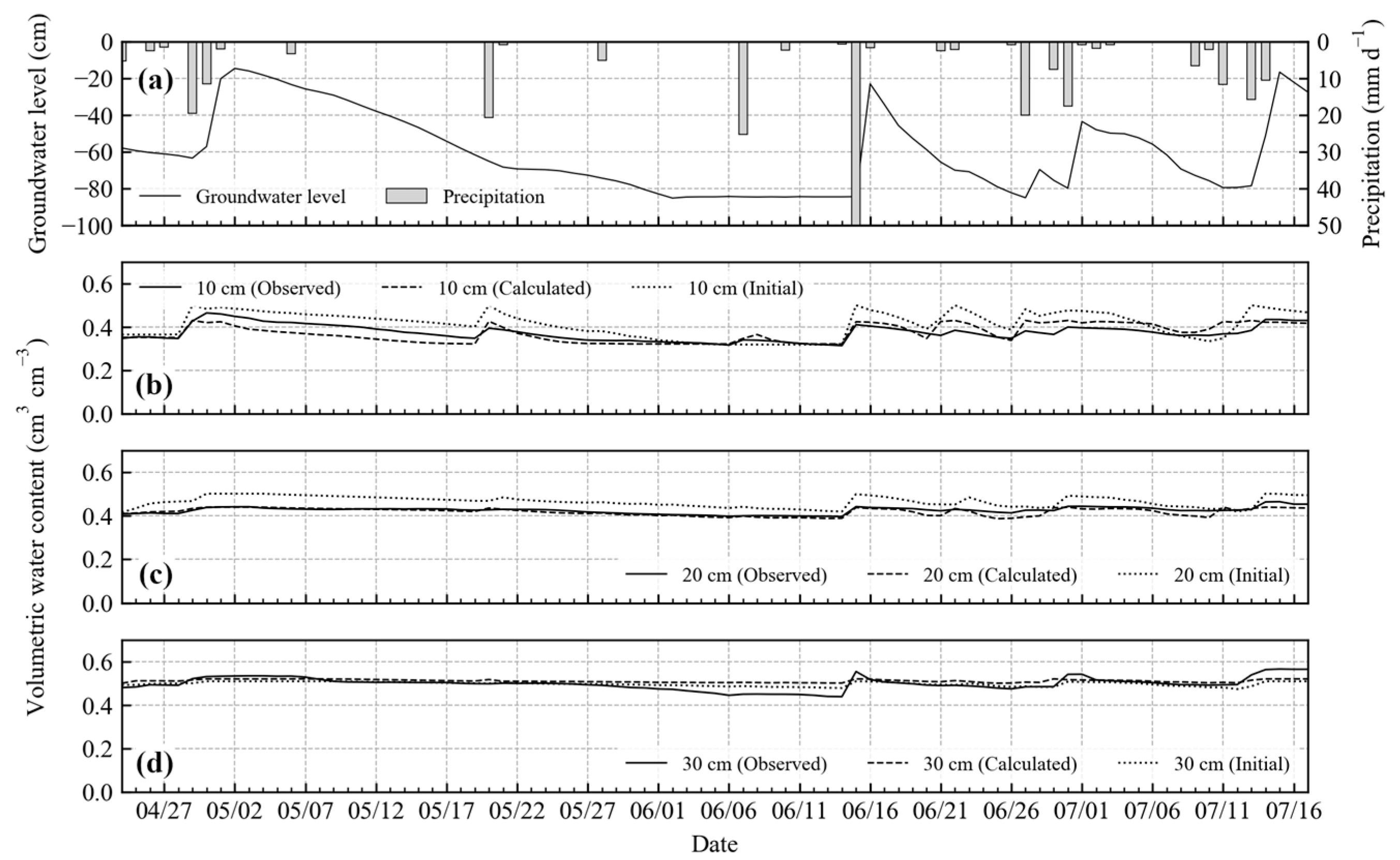
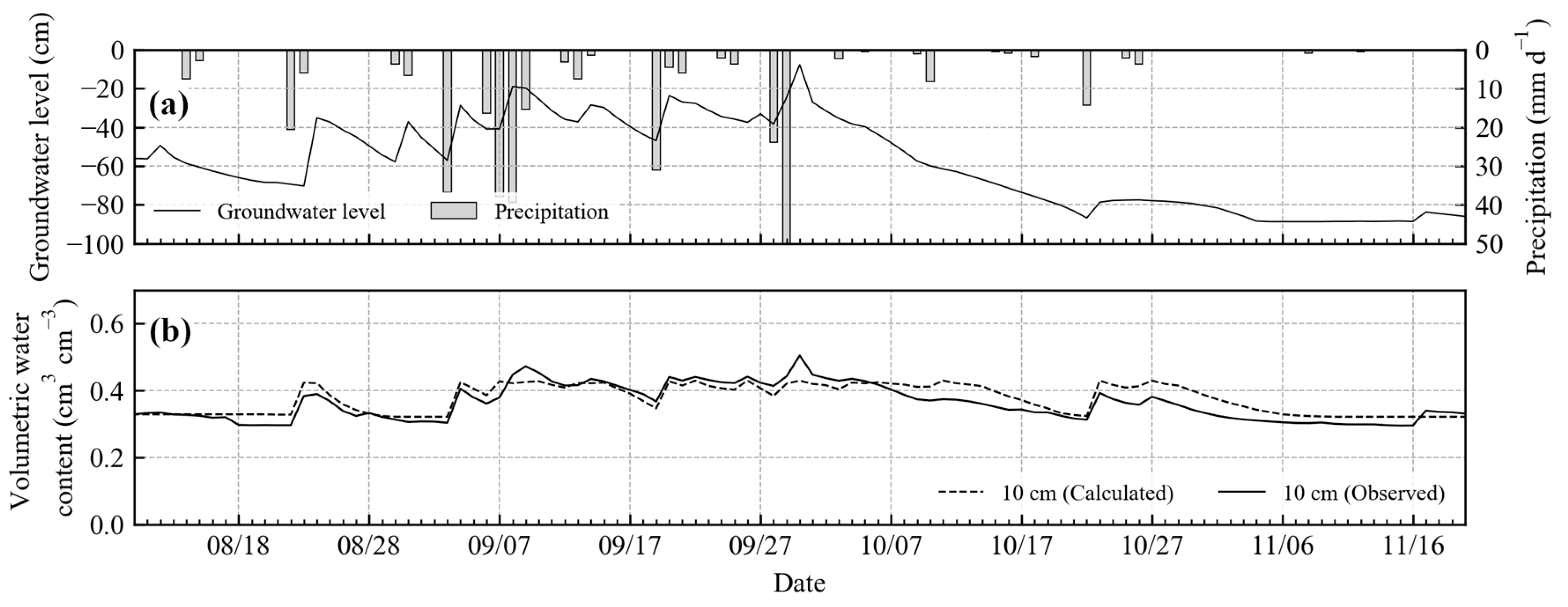
3.2. Model Validation

The SWAP model with optimized parameters was able to simulate the volumetric water content under significantly different weather conditions. Figure 6a shows the groundwater level and precipitation in the validation plot in 2018; precipitation intensity and groundwater level were higher in 2018 than in 2019 (Figure 4a). Before 29 September 2018, the groundwater level was relatively high, and precipitation occurred frequently. The maximum daily precipitation (82.7 mm d⁻¹) occurred on 29 September 2018. Thereafter, the groundwater level gradually decreased to its lowest value (−90 cm), and precipitation became less frequent. Figure 6b shows the temporal changes in θ_obs and θ_cal at a depth of 10 cm: the trends in θ_cal and θ_obs were matched; both values changed with the precipitation. The RMSE between θ_cal and θ_obs was 0.029 cm³ cm⁻³. This result indicates that, even with high levels of precipitation and groundwater, the model was able to reproduce actual volumetric water content using our calibrated parameters.

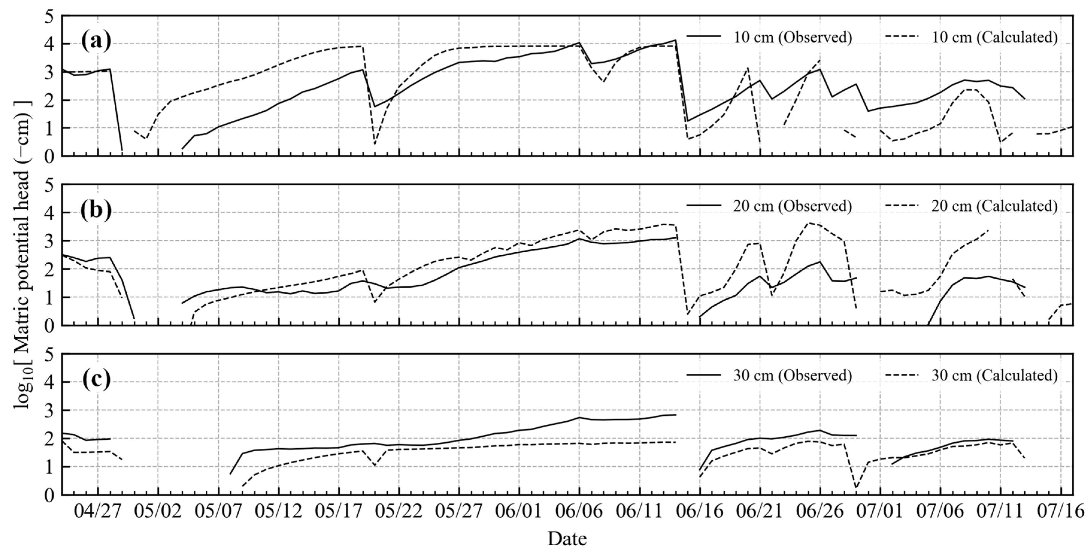
3.3. Change in Matric Potential in the Calibration Plot

Calculated matric potential head (h_cal) in the calibration plot captured the trend of change in observed value (h_obs) except after 15 June 2019, when precipitation was more frequent (Figure 4a and Figure 7). We excluded positive pressure head in Figure 6. Before 15 June 2019, h_cal at a depth of 10 cm changed similarly to h_obs except between 30 April and 19 May 2019. In this period, h_cal was almost 10 times higher than h_obs; this reflected lower θ_cal than θ_obs in the same period (Figure 4b and Figure 7a). At depths of 20 and 30 cm, the changes in h_obs and h_cal were similar. After 27 May 2019, h_obs at a depth of 30 cm became larger than h_cal due to the decrease in θ_obs in this period (Figure 4d and Figure 7c). Except at a depth of 30 cm, h_cal differed from h_obs after 15 June 2019. At a depth of 10 cm, h_cal tended to be smaller than h_obs; h_cal was larger than h_obs at a depth of 20 cm. The RMSEs between h_obs and h_cal at depths of 10, 20, and 30 cm were 1.0, 0.7, and 0.6 log₁₀(−cm), respectively. These results indicate that the calculated water stress after 15 June 2019 might contain larger error than that before the day.

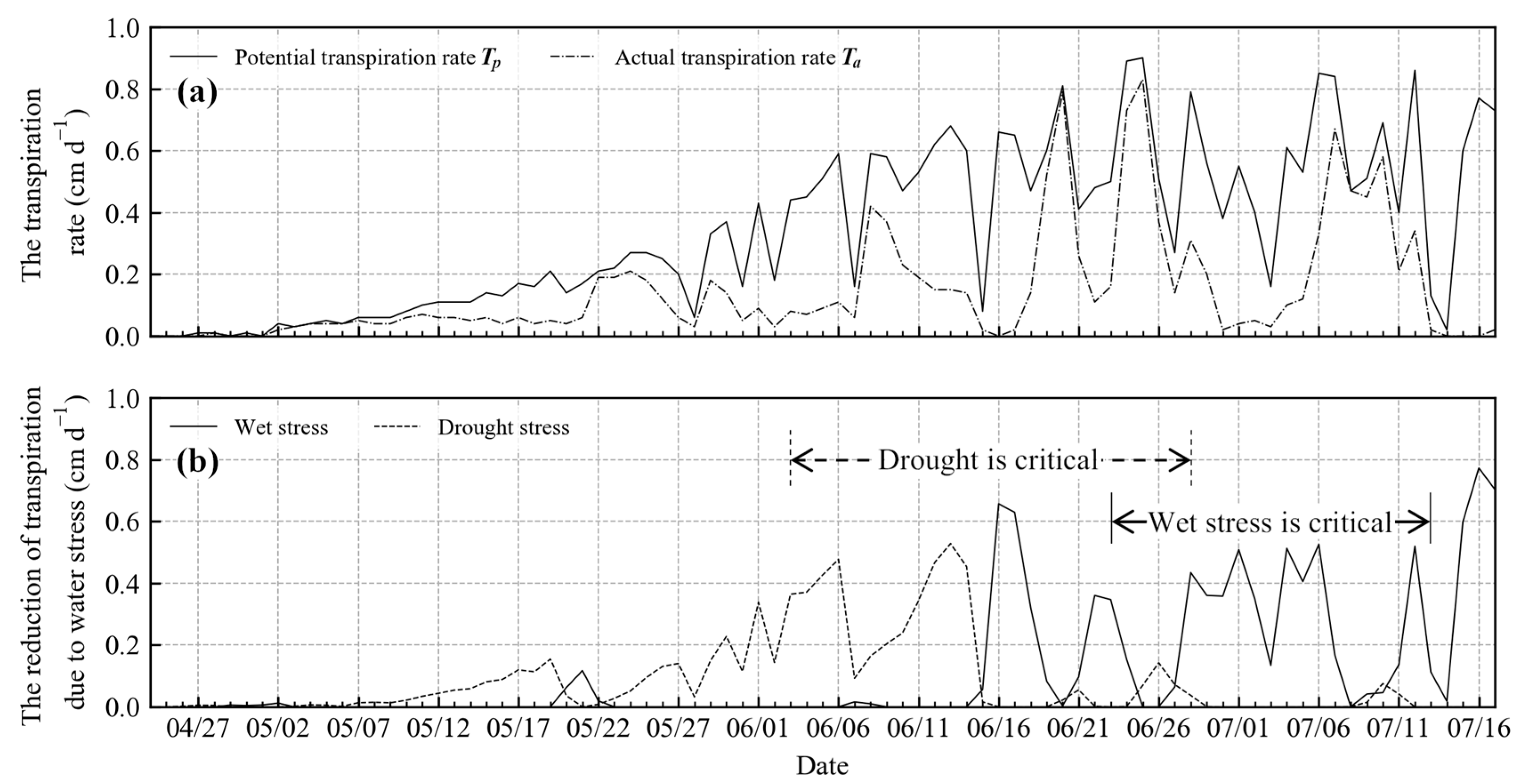
3.4. Water Stress under Actual Conditions

Our simulation revealed that maize cultivation under actual conditions would be highly likely to suffer from water stress. Figure 8a shows T_p and T_a in the calibration plot in 2019 as estimated by the SWAP model. T_a was significantly lower than T_p during most of the simulation period, reaching an approximate extreme of only 20% of T_p. From 28 May to 15 June 2019, less precipitation occurred, and the groundwater level was low (Figure 4a). Thus, the difference between T_p and T_a might have been induced by dry conditions. After 15 June 2019, groundwater level and precipitation increased; T_a during this period may have decreased due to the wet conditions. However, several zero-precipitation days (namely, 17–20 June, 23–25 June, and 4–8 July 2019) occurred during this period. Although the comparison between T_p and T_a indicates that water stress occurred, we could not distinguish whether it was drought or wet stress that affected T_a.

Separate evaluations of drought and wet stresses are likely to be necessary when determining appropriate adaptation measures. Figure 8b shows the drought and wet stresses separately, highlighting the critical growth periods for drought and wet stresses [3,4]. As shown in Figure 4a and Figure 8b, little rain fell until 15 June 2019, and drought stress increased during this period. The maximum drought stress level occurred on 13 June 2019. Wet stress predominated after 15 June 2019, when precipitation was more frequent. Moreover, the highest groundwater levels appeared on 16 June, 12 July, and 15 July 2019, which could have induced wet stress. The two highest levels of wet stress occurred on 16 June and 16 July 2019. Figure 8b indicates that under the actual conditions, drought and wet stresses appeared between 3 and 13 June 2019 (40–50 days after emergence) and between 23 June and 13 July 2019 (60–80 days after emergence), respectively. This implies that the actual conditions were disadvantageous for maize growth in terms of water stress. We note that the second largest peak of wet stress on 16 June 2019 may affect crop growth adversely even the stress occurred in the critical period for drought stress (Figure 8b).

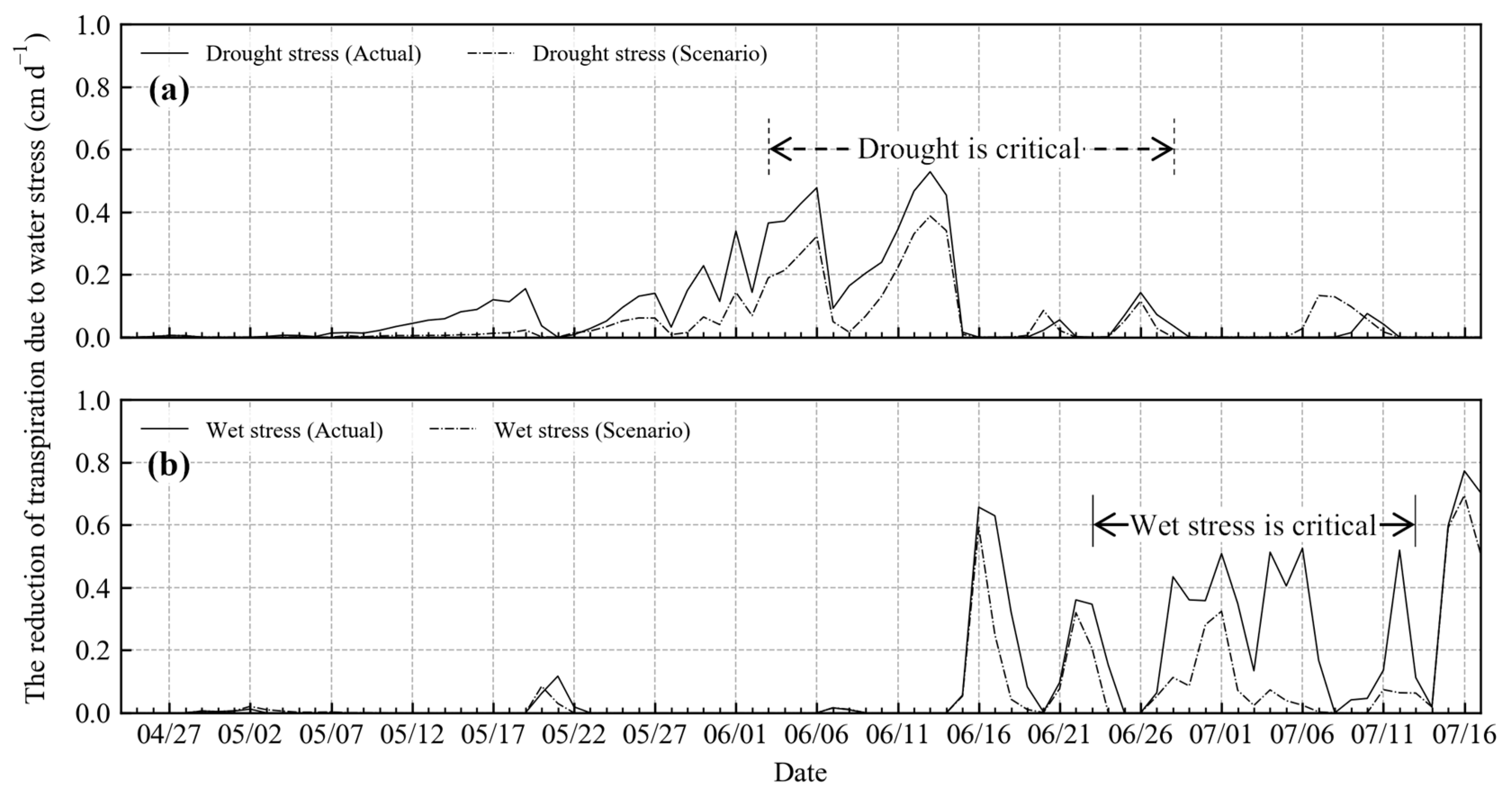
3.5. Illustrative Example: Reduction of Water Stress by Changing Tillage Depth

Figure 9, panels a and b, show the drought and wet stresses for the actual and scenario conditions, respectively. In the scenario, drought stress was lower than under actual conditions for most of the simulation period. From 3 to 15 June 2019, when drought stress under actual conditions was relatively high in relation to the relevant critical growth period (defined as the drought-dominant period), the stress under the scenario conditions was 33%–75% of that under actual conditions (Figure 9a). Wet stress under the scenario conditions was also lower than, or the same as, that under actual conditions. In the growth period during which wet stress was critical, stress under scenario conditions was 10%–82% of that under actual conditions (Figure 9b). These results suggest that making the tillage depth 11 cm deeper tends to reduce both forms of stress during the maize critical growth periods.

The water stress at depths of 10 and 20 cm differed between the actual and scenario conditions (

Table 6. Average volumetric water content per day and the number of days under stress, under actual and scenario conditions.

Depth	Condition	Drought-Dominant Period (3–15 June 2019; 12 days)		Wet Stress Critical Period (23 June–13 July 2019; 20 days)
		Average Volumetric Water Content (cm3 cm−3)	Stress Occurrence Days	Average Volumetric Water Content (cm3 cm−3)	Stress Occurrence Days
10 cm	Actual	0.330	12	0.405	13
	Scenario	0.331	12	0.375	4
20 cm	Actual	0.393	12	0.416	8
	Scenario	0.380	0	0.390	1

The “drought-dominant period” is the period when drought stress was significant and the maize growth phase was drought-sensitive (3–28 June 2019). Stress occurrence days were calculated based on Figure 5 and volumetric water content under actual and scenario conditions (data not shown).

). Throughout the drought-dominant period, drought stress occurred at a depth of 10 cm under both conditions. At a depth of 20 cm, however, although the average volumetric water content under scenario conditions was lower than under actual conditions, it was in the no-stress range, as indicated by the soil water retention curve (Figure 5a). During the wet stress critical period, stress tended to occur more often at a depth of 10 cm than at 20 cm (Table 6). Wet stress occurred on fewer days under scenario than actual conditions at both depths. These results indicate that the scenario conditions probably mitigate water stress at depths of 10 and 20 cm. Moreover, water stress varied with depth; by evaluating drought and wet stresses at different depths, future studies could identify the critical layer or depth for crop growth under actual and scenario conditions.

4. Conclusions

In this study, the drought and wet stresses in a converted maize field in Okayama, Japan, were evaluated using a SWAP model. The model was calibrated and validated using data from field observations. The water stress under actual and scenario (tillage depth 11 cm deeper) conditions were then estimated. Our study revealed that (1) drought and wet stresses appeared within the relevant critical growth stages of maize, under actual conditions; (2) water stress under the scenario condition tended to be lower than under actual conditions, with drought and wet stresses 33%–75% and 10%–82% of those under actual conditions, respectively; (3) water stress between soil depths of 10 and 20 cm was lower under the scenario conditions than under the actual conditions. Those results indicate that deeper tillage may mitigate both drought and wet stresses. We hypothesize that by evaluating drought and wet stresses at different depths, we can identify the critical layer or depth for crop growth; this will promote further reduction in water-related crop damage in converted fields. The method presented here can be applied to fields with suboptimal water conditions, and may enhance yield. Further, we believe that our study will support precise stress control management, and boost crop yield and quality, when combined with precision farming applications in converted fields.

References

1. Hashimoto, I. Studies on irrigation management and water requirements of upland fields converted from paddy fields and those of protected cultivation fields. Bull. Ishikawa Agric. Coll. 1999, 29, 1–28. [Google Scholar]
2. Taki, S.; Kujira, Y. Effects of different soil condition on growth of soybean cv. Enrei. Hokuriku Crop Sci. 2009, 44, 41–45, (In Japanese with English abstract). [Google Scholar]
3. Çakir, R. Effect of water stress at different development stages on vegetative and reproductive growth of corn. Field Crop. Res. 2004, 89, 1–16. [Google Scholar] [CrossRef]
4. Kanwar, R.S.; Baker, J.L.; Mukhtar, S. Excessive soil water effects at various stages of development on the growth and yield of corn. Trans. ASAE 1988, 31, 133–141. [Google Scholar] [CrossRef] [Green Version]
5. van Dam, J.S.; Huygen, J.; Wesseling, J.G.; Feddes, R.A.; Kabat, P.; van Walsum, P.E.V.; Groenendijk, P.; van Diepen, C.A. Theory of SWAP Version 2.0; Simulation of Water Flow, Solute Transport and Plant Growth in the Soil-Water-Atmosphere-Plant Environment; DLO Winand Staring Centre: Wageningen, The Netherlands, 1997. [Google Scholar]
6. Kroes, J.G.; van Dam, J.C.; Bartholomeus, R.P.; Groenendijk, P.; Heinen, M.; Hendriks, R.F.A.; Mulder, H.M.; Supit, I.; van Walsum, P.E.V. SWAP Version 4. Theory Description and User Manual; Wageningen Environmental Research: Wageningen, The Netherlands, 2017. [Google Scholar]
7. Anan, M.; Hamada, K.; Yuge, K. Risk prediction of water stress by rainfall and continuous drought weather in reclaimed crop field. J. Rainwater Catchment Syst. 2015, 21, 37–42, (In Japanese with English abstract). [Google Scholar] [CrossRef] [Green Version]
8. Yuge, K.; Hamada, K.; Anan, M.; Hamagami, K.; van Dam, J.S.; Kroes, J.G. Evaluation of water stress and optimization of irrigation regime at crop fields in polder. IDRE J. 2018, 306, I_55–I_62, (In Japanese with English abstract). [Google Scholar] [CrossRef]
9. Mualem, Y. A new model for predicting the hydraulic conductivity of unsaturated porous media. Water Resour. Res. 1976, 12, 513–522. [Google Scholar] [CrossRef] [Green Version]
10. van Genuchten, M.T. A closed-form equation for predicting the hydraulic conductivity of unsaturated soils. Soil Sci. Soc. Am. J. 1980, 44, 892–898. [Google Scholar] [CrossRef] [Green Version]
11. Penman, H.L. Natural evaporation from open water, bare soil, and grass. Proc. R. Soc. A 1948, 193, 120–146. [Google Scholar] [CrossRef] [Green Version]
12. Monteith, J.L. Evaporation and Environment. In The State and Movement of Water in Living Organisms; Fogg, G.E., Ed.; Cambridge University Press: Cambridge, UK, 1965; pp. 205–234. [Google Scholar]
13. Feddes, R.A.; Kowalik, P.J.; Zaradny, H. Simulation of Field Water Use and Crop Yield; Wiley: New York, NY, USA, 1978. [Google Scholar]
14. Kanda, T.; Takata, Y.; Kohyama, K.; Ohkura, T.; Maejima, Y.; Wakabayashi, S.; Obara, H. New soil maps of Japan based on the comprehensive soil classification system of Japan—First approximation and its application to the world reference base for soil resources 2006. Jpn. Agric. Res. Q. 2018, 52, 285–292. [Google Scholar] [CrossRef] [Green Version]
15. Black, C.A.; Evans, D.D.; Ensminger, L.E.; White, J.L.; Clark, F.E. (Eds.) Methods of Soil Analysis. Part 1. Physical and Mineralogical Properties, Including Statistics of Measurement and Sampling; American Society of Agronomy Inc.: Madison, WI, USA, 1965. [Google Scholar]
16. Tomohiro, N. Control of water erosion loss of soils using appropriate surface management in Tanzania and Cameroon. In Soils, Ecosystems Processes, and Agricultural Development: Tropical Asia and Sub-Saharan Africa; Funakawa, S., Ed.; Springer: Tokyo, Japan, 2017; p. 344. [Google Scholar]
17. Jury, W.A.; Horton, R. Soil Physics, 6th ed.; John Wiley & Sons: New York, NY, USA, 2004. [Google Scholar]
18. Ono, H.; Sasaki, K.; Ohara, G.; Nakazono, K. Development of grid square air temperature and precipitation data compiled from observed, forecasted, and climatic normal data. Clim. Biosph. 2016, 16, 71–79, (In Japanese with English abstract). [Google Scholar] [CrossRef] [Green Version]
19. Maddonni, G.A.; Otegui, M.E. Leaf area, light interception, and crop development in maize. Field Crop. Res. 1996, 48, 81–87. [Google Scholar] [CrossRef]
20. Wesseling, J.G.; Elbers, J.A.; Kabat, P.; van den Broek, B.J. SWATRE: Instructions for Input. Internal Note; Winand Staring Centre: Wageningen, The Netherlands, 1991. [Google Scholar]
21. Jiang, J.; Feng, S.; Huo, Z.; Zhao, Z.; Jia, B. Application of the SWAP model to simulate water-salt transport under deficit irrigation with saline water. Math. Comput. Model. 2011, 54, 902–911. [Google Scholar] [CrossRef]
22. Jiang, J.; Feng, S.; Ma, J.; Huo, Z.; Zhang, C. Irrigation management for spring maize grown on saline soil based on SWAP model. Field Crop. Res. 2016, 196, 85–97. [Google Scholar] [CrossRef]
23. Kumar, P.; Sarangi, A.; Singh, D.K.; Parihar, S.S.; Sahoo, R.N. Simulation of salt dynamics in the root zone and yield of wheat crop under irrigated saline regimes using SWAP model. Agric. Water Manag. 2015, 148, 72–83. [Google Scholar] [CrossRef]
24. Crescimanno, G.; Garofalo, P. Management of irrigation with saline water in cracking clay soils. Soil Sci. Soc. Am. J. 2006, 70, 1774–1787. [Google Scholar] [CrossRef]
25. Strudley, M.W.; Green, T.R.; Ascugh II, J.C. Tillage effects on soil hydraulic properties in space and time: State of the science. Soil Till. Res. 2008, 99, 4–48. [Google Scholar] [CrossRef]
26. Or, D.; Leij, F.J.; Snyder, V.; Ghezzehei, T.A. Stochastic model for posttillage soil pore space evolution. Water Resour. Res. 2000, 36, 1641–1652. [Google Scholar] [CrossRef] [Green Version]
27. Kita, D.; Tarumi, H.; Mori, H.; Kawaguchi, K. A new theory of the function of bentonite in suppressing the water percolation through soils. Jpn. J. Soc. Soil Sci. Plant Nutr. 1964, 35, 47–52. (In Japanese) [Google Scholar]
Figure 1. The reduction factor for excessive wet and dry conditions, αrw, as a function of matric potential head; h1, h2, h3, and h4 are critical pressure heads (−cm); h3 is between h3h and h3l values for high and low transpiration rates, respectively; h3 depends on the water demand of the atmosphere (Tlow and Thigh) and varies with the potential transpiration rate Tp. Wet stress occurs when wetter than h2, whereas drought stress occurs when drier than h3.
Water 12 01363 g001
Figure 2. The converted field in this study. The field was divided into a calibration plot and a validation plot.
Water 12 01363 g002
Figure 3. Schematic diagram of the experimental plot. (a) Horizontal view; (b) vertical view.
Water 12 01363 g003
Figure 4. Volumetric water content in the calibration plot in 2019. (a) Groundwater level and precipitation; (bd) results at depths of 10, 20, and 30 cm, respectively. The maximum daily precipitation, 51.7 mm d−1, occurred on 15 June 2019. The results with initial and calibrated soil hydraulic parameters were generated using the data in Table 4 and Table 5, respectively.
Water 12 01363 g004
Figure 5. The analytical soil water retention curves generated by initial and calibrated Mualem–van Genuchten parameters. (ac) Results for layers 1, 2, and 3, respectively. The grey area represents the zero-water-stress zone; drought or wet stresses occur outside this area. In the scenario condition, layers 1 and 2 used the calibrated soil water retention curve of layer 1.
Water 12 01363 g005
Figure 6. Volumetric water content in the validation plot in 2018. (a) Groundwater level and precipitation; (b) θcal and θobs at a depth of 10 cm. The maximum daily precipitation, 82.7 mm d−1, occurred on 29 September 2018.
Water 12 01363 g006
Figure 7. Matric potential head in the calibration plot in 2019. (ac) Results at depths of 10, 20, and 30 cm, respectively. Those results were converted from observed and calculated volumetric water content by using calibrated Mualem–van Genuchten parameters (Table 5). We excluded data that showed positive values.
Water 12 01363 g007
Figure 8. Potential and actual transpiration rates and water stress under actual conditions in 2019. (a) Transpiration rates; (b) water stress. The critical growth periods for drought and wet stresses were defined based on Çakir [3] and Kanwar et al. [4].
Water 12 01363 g008
Figure 9. Drought and wet stresses under actual and scenario conditions in 2019. (a) Drought stress; (b) wet stress. The critical growth periods for drought and wet stresses were defined based on Çakir [3] and Kanwar et al. [4].
Water 12 01363 g009