Vegetation Alters Soil Water Drainage and Retention of Replicate Rain Gardens

Abstract

Rain gardens are residential bioretention practices widely used to manage urban runoff, yet their design as plant-soil systems lacks understanding. We hypothesized that vegetative treatment (turfgrass, prairie, and shrubs, plus a non-vegetated control) would alter the volume and rate of drainage from 12 replicate mesocosms (i.e., rain gardens) through changes to the belowground system. Roof runoff was collected on-site and distributed equally among the mesocosms following natural rain events for two growing seasons. We monitored stormwater input, drainage output, and soil moisture to assess differences in hydrology by treatment, explained by indices of soil structural development (infiltration, saturated hydraulic conductivity, soil water retention). Drainage volume and response dynamics differed as predicted by vegetative treatment in support of our hypothesis. The greatest reductions in drainage volume were observed beneath shrubs and prairie following smaller stormwater inputs, and accelerated drainage responses were observed beneath turfgrass following larger stormwater inputs. Differences in infiltration, saturated hydraulic conductivity, and plant-induced changes in antecedent soil moisture among vegetative treatments help explain these plant-mediated drainage responses. This study shows that plants can alter the hydrologic dynamics of rain gardens and thus are a critical component of the design and intent of these plant-soil systems.

1. Introduction

Urbanization transforms the land surface and alters the pre-development hydrologic cycle, and these changes amplify the need for surface water management. Since the 1970s, urban land development has led to declines in soil-water recharge by as much as 80% [1]. The resulting runoff typically yields increased volume, increased flow rates, and shorter flow durations than the predevelopment hydrology. For example, a 10% increase in impervious surfaces within a watershed outside of New York, NY, yielded stormwater with a three-fold greater peak flow rate compared with a nearby undeveloped watershed; the flow duration was also shortened from approximately 75 to >20 min [2]. The remaining pervious areas, such as beneath street trees and turfgrass lawn, can also exhibit decreased infiltration if soil compaction occurred during land development [3,4,5]. Yet, urban vegetation may help mitigate the environmental consequences of urbanization [6,7,8]. One popular solution to restore infiltration in urban areas is the best management practice known as a bioretention cell or rain garden; these vegetated catchments are specifically designed to collect, store, and infiltrate stormwater and thus dispel the large volumes and flow rates of surface runoff [9].

The installation of bioretention areas to intercept stormwater continues to outpace our understanding of these practices as plant–soil systems. Research on bioretention areas has focused on catchment size [10,11], the composition of different soil mixtures [12,13], and internal design features that control the flow of water and potential pollutants [14,15]. Differences in vegetation and soil properties were associated with changes in bioretention cell performance and water chemistry [16,17,18,19,20], but we are only beginning to appreciate the role of plants as altering soil hydrologic processes in bioretention systems [21,22]. Understanding how plants alter soil physical properties and drainage of these bioretention systems will guide how we use them for pollutant removal. Moreover, the plants used for bioretention range from macrophytes to water-tolerant flowering forbs, grasses, shrubs, or trees as recommended by numerous “how to” guides that offer lists of species for these systems [23]. This variety in vegetation choice has helped popularize bioretention around the world, but it confounds our ability to quantify their hydrologic impact and assumes little to no difference related to plant type and behavior. Thus, the biophysical role of vegetation remains unclear in the context of bioretention [24] because no study has tested the effect of vegetation type on real-time dynamics of soil water in a controlled experiment of replicated systems.

Plants are critical to the function of bioretention systems not only through their direct uptake of soil water but also through their indirect role in soil structural development. Soil structure describes the arrangement of solids and voids (pores) within a volume of soil where the amount and distribution of pore size controls such characteristics as soil water infiltration, retention, redistribution, and conductivity [25]. The capacity for plants to build, alter, and stabilize soil structure depends on their root architecture and belowground productivity [26], as roots physically enmesh soil aggregates [27], create pores in soil [28], and buffer the soil against slaking and infilling [29,30]. The effects of plants on soil pore spaces over time together embody a structural domain of soil porosity, enhancing the textural domain of soil porosity that was determined by the physical composition of the soil mixture [31]. Ultimately, these plant-induced changes in soil structure modify soil hydrology through improved soil pore connectivity. Increased rates of soil saturated hydraulic conductivity (K_s) observed under prairie plants with extensive root development exemplify this relationship [32,33,34].

We hypothesize the volume and flow rate of drainage from bioretention systems will differ by vegetative treatment and size of stormwater input, and that these differences can be explained by plant-soil interactions that control the retention and movement of soil water. To test this hypothesis, we first sought to quantify the direct effect of vegetation type on the drainage response of replicated bioretention mesocosms that receive rooftop stormwater generated by natural rain events. Second, we used indices of soil structural development (infiltration rate, K_s, and soil water retention) to evaluate changes in porosity beneath each vegetation type.

2. Materials and Methods

2.1. Site Description

This research was conducted at an experimental facility located in the town of Verona, part of the greater Madison area in south-central Wisconsin (43°09′ N, 89°37′ W). The greater Madison area is the center for rapid urban growth and development in Dane County, currently supporting over 300,000 people, or 65% of the population county-wide. Groundwater is the primary source of potable water, and land use planners, therefore, support local practices that infiltrate stormwater [35]. The region is characterized by a northern temperate climate with mean summer and winter temperatures of 21 °C and −6 °C, respectively, and a normal annual precipitation of 837 mm [36]. In the two years of study, the mean summer air temperature was 19.4 °C and 22.5 °C, respectively, and the total annual rainfall each year was 60 mm greater than normal [36].

2.2. Experimental Design

Twelve rain gardens were constructed as mesocosms to test the effects of vegetation type on hydrology and soil development by varying only the vegetative component. The experiment used a randomized complete block design of three blocks with four vegetative treatments per block: bare soil (control), turfgrass sod, wet-mesic prairie vegetation (mix of 18 species including both grasses and flowering forbs), and landscaping shrubs (a mix of 6 water-tolerant species) (

Table 1. Plant species in the turfgrass, prairie, and shrub vegetative treatments.

Latin Name	Family Name	Common Name
Turfgrass Treatment
Poa pratensis	Poaceae	Kentucky bluegrass
Prairie Treatment
Andropogon gerardii	Poaceae	Big bluestem
Asclepias incarnata	Asclepiadaceae	Swamp milkweed
Baptisia bracteata	Fabaceae	Longbract wild indigo
Boltonia asteroides	Asteraceae	White doll’s daisy
Carex vulpinoidea	Cyperaceae	Fox sedge
Echinacea purpurea	Asteraceae	Eastern purple coneflower
Echinacea pallida	Asteraceae	Pale purple coneflower
Eupatorium perfoliatum	Asteraceae	Common boneset
Heliopsis helianthoides	Asteraceae	Smooth oxeye sunflower
Liatris pycnostachya	Asteraceae	Prairie blazing star
Monarda fistulosa	Lamiaceae	Wild bergamot
Oligoneuron ohioense	Asteraceae	Ohio goldenrod
Panicum virgatum	Poaceae	Switchgrass
Parthenium integrifolium	Asteraceae	Wild quinine
Penstemon calycosus	Scrophulariaceae	Longsepal beardtongue
Ratibida pinnata	Asteraceae	Pinnate prairie coneflower
Rudbeckia hirta	Asteraceae	Blackeyed Susan
Symphyotrichum novae-angliae	Asteraceae	New England aster
Veronicastrum virginicum	Scrophulariaceae	Culver’s root
Shrub Treatment
Cornus sericea “Isanti”	Cornaceae	Red osier dogwood
Ilex verticillata “winter red”	Aquifoliaceae	Common winterberry
Photinia melanocarpa	Rosaceae	Black chokeberry
Salix purpurea ”Gracilis”	Salicaceae	Purpleosier willow
Viburnum dentatum	Caprifoliaceae	Southern arrowwood
Viburnum opulus	Caprifoliaceae	American cranberrybush

). These three plant assemblages were selected to represent the range in plant types used for bioretention [14,37].

All mesocosms were constructed of wooden frames of equal size (2.44 m by 2.44 m by the total depth of 1.22 m) and filled with a soil mixture (ratio of 3:1:6 by volume of topsoil, compost, and sand, respectively) that is recommended locally for bioretention [38]. This soil mixture was 43% sand, 40% silt, and 17% clay by mass (determined through textural analysis with hydrometer after hydrogen peroxide pretreatment [39,40]) and 6% soil organic matter (by loss on ignition [41]). The soil mixture was not evaluated for chemical properties. The soil area per mesocosm (5.9 m²) represented 17% of its respective contributing roof area (34.8 m²) per sizing recommendations [10,42]. Mesocosms were designed to hold roof water from a typical storm event of 25.4-mm rainfall accumulation in south-central Wisconsin (e.g., storms with 2-h duration and 3-mo frequency [43]).

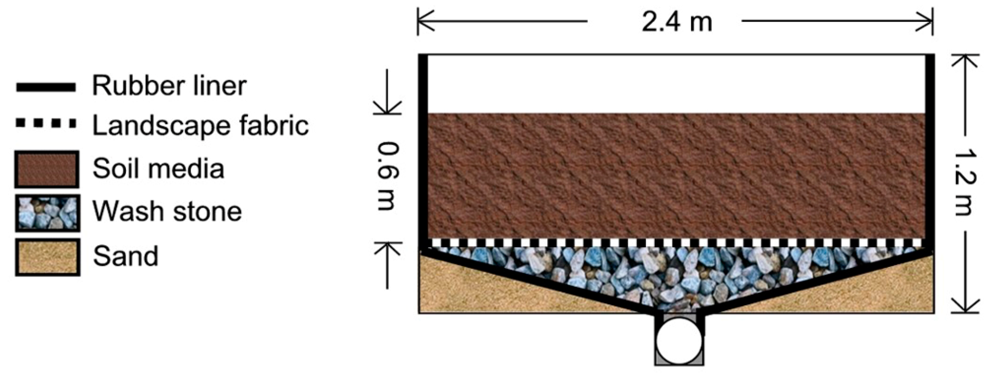
Each mesocosm was an individual, closed system that drained freely to a central tile drain [16,20]. Each consisted of a wooden frame with a 30 mil rubber liner along the bottom and sidewalls, a bed of wash stone (5 cm diameter) below a layer of landscape fabric, and a rooting zone of soil media (Figure 1). Two rings of bentonite clay were placed along the interior perimeter of each mesocosm at depths of 0.3 and 0.5 m to prevent preferential flow along the interior of the side walls. The effective rooting depth was 0.6 m. A central PVC pipe directed all drainage to a flow monitoring station. Water stored in the internal design features (e.g., wash stone) did not change over time within an individual system or treatment [16,20,44]. Each mesocosm had a closed hydrologic budget in which 96 ± 6% of the input water volume was collected as drainage, stored in the soil, or lost via evapotranspiration [44]. The 12 mesocosms were positioned in the landscape such that the planted areas were above flow monitoring stations located behind wooden retaining walls (Figure 2). The four mesocosms within each block were randomly assigned a vegetative treatment.

The mesocosms were established in 2005 using plant stock from local nurseries. Turfgrass mesocosms were planted with Kentucky bluegrass sod (Poa pratensis L.) and maintained with hand-shears to a height of 7 cm. Prairie mesocosms were initially planted with plugs on a grid of 0.3-m spacing but spread to 80% soil coverage. Shrub mesocosms were planted with six shrubs, one per species, spaced equally apart from one another. Control (bare soil) mesocosms were raked annually in April and covered with fiberglass window screen to reduce the erosive impact of rainfall and the formation of surface crusts; these screens were removed before and replaced after stormwater applications. All mesocosms were maintained by hand-weeding.

2.3. Stormwater Inputs

The study site was equipped to collect and distribute natural rainfall to the mesocosms to simulate the episodic inputs of stormwater generated by impervious surfaces. Two tanks, one on either side of a metal-roofed shed, together stored 25.4 mm of rainfall over a total roof area of 417.6 m², which was then divided equally among the 12 mesocosms. With both tanks full, each mesocosm received 127.3 mm (751 L) of the collected stormwater. The volume of stormwater applied to the mesocosms was quantified via a digital in-line flow meter (±0.04 L, model 825, Systems, Tuthill Corporation, Burr Ridge, IL, USA) at a constant rate of inflow of 192 mm h⁻¹ (1133 L h⁻¹); this rate was selected to enable all 12 applications (one per mesocosm per rain event) to be completed on the same day. Perforated PVC tubes spanning the length and width of each mesocosm distributed stormwater across the soil surface [16].

For each natural rain event, the total volume of rainfall collected from the roof was distributed equally among all mesocosms. The stormwater simulations (hereafter referred to as applications) on a given day were applied randomly first by block and then by mesocosm within the block. Stormwater applications were completed within 48 h of the preceding rain event, with few exceptions (e.g., when the weather forecast predicted additional rain within the next 24 h, we delayed the applications until the next dry day). We waited for mesocosm drainage generated by rainfall (if any) to return to the measurement threshold (defined as flow <0.25 mm h⁻¹). Thus, this study quantified drainage responses following inputs of stormwater in accordance with the stochastic distribution of rainfall over two growing seasons (May to September). This is different from previous work in which rainfall simulations were completed on a pre-determined schedule (such as in the summer months only [20]).

In total, 41 stormwater applications were applied to the 12 mesocosms over two growing seasons (

Table 2. Stormwater applications (mm) applied over two years of monitoring. Input data were separated into three size classes: small (8–50 mm), medium (51–90 mm), and large (91–130 mm). An input of 127.3 mm applied over 5.9 m² soil area equals an applied volume of 751 L.

Small Inputs		Medium Inputs		Large Inputs
Input	Date	Input	Date	Input	Date
(mm)		(mm)		(mm)
Year 1		Year 1		Year 1
8.3	17 June	50.9	1 August	111.4	22 July
9.5	3 August	54.1	21 August	127.3	20 June
12.7	18 August	76.4	9 June	127.3	9 August
15.9	14 June	82.8	25 July	Year 2
15.9	22 June	84.7	11 July	95.5	24 June
16.6	9 July	Year 2		127.3	27 April
19.1	29 June	50.9	18 June	127.3	14 May
19.1	10 August	63.7	9 June	127.3	27 May
19.1	26 August	82.8	22 June	127.3	7 June
28.6	28 August	82.8	15 July	127.3	16 June
35.0	15 July	89.1	8 July	127.3	28 June
47.7	10 June			127.3	26 July
47.7	1 September			127.3	10 August
Year 2				127.3	16 August
12.7	19 July
24.2	24 May
25.5	25 August
31.8	3 June
38.2	29 July

). We applied the maximum amount of collected stormwater (127.3 mm per mesocosm) on two dates in year 1 and on nine dates in year 2. The reference treatment (non-vegetated controls) and turfgrass treatment produced a drainage response on every application date during the study except one date. When the smallest input (8.3 mm) was applied, none of the mesocosms produced drainage responses above the measurement threshold. The prairie and shrub treatments had six additional “no flow” situations, and the amount of stormwater input applied on these six dates ranged from 9.5–19.1 mm.

2.4. Drainage and Climate Monitoring

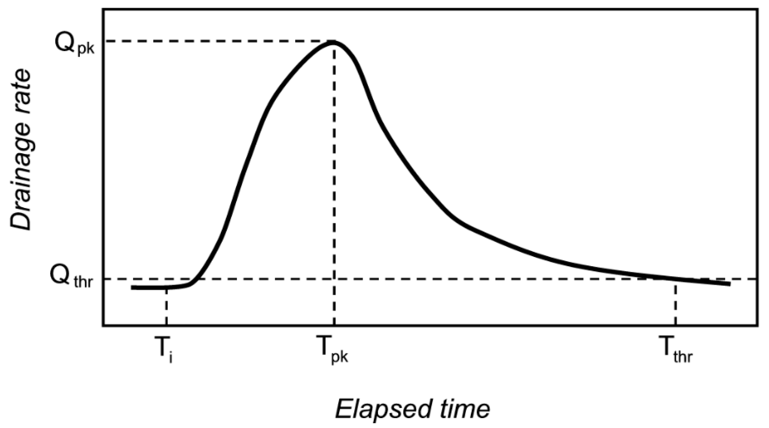
The timing and magnitude of drainage were measured with a flow monitoring station located at the outflow point of each mesocosm. A tipping-bucket (0.5 L tip⁻¹) wired to a data logger (CR1000, Campbell Scientific Inc., Logan, UT, USA) recorded drainage flow rates in 5-min intervals. We characterized the drainage response of each mesocosm per stormwater event, starting from the time of stormwater inflow (T_i) and stopping (T_thr) when the flow was again 0.25 mm h⁻¹ (Q_thr); we quantified the drainage volume (% of input), the lag time to peak flow defined here as T_i to T_pk (min), the peak flow rate of drainage (Q_pk, mm h⁻¹), and the response duration defined here as T_i to T_thr (h) (Figure 3). In cases when drainage was less than our threshold, the response was considered a ‘no flow’ situation, and we assigned values of zero to drainage volume, lag time, peak flow, and response duration. The flow response to rainfall itself was not tested in this study because very few rain events generated drainage. Thus, we report data for only the drainage response of the mesocosms generated by stormwater inputs.

The study site was instrumented to continually monitor soil moisture and weather. Two soil moisture sensors were installed per mesocosm at depths of 0–0.15 and 0.30–0.45 m (CS616, Campbell Scientific Inc., Logan, UT, USA). The soil moisture sensors were calibrated to the specific soil mixture used in the mesocosms and tested for accuracy in the field [44]. Soil moisture (m³ m⁻³) at each depth was monitored at 15-min intervals over the growing season (May–September), and antecedent soil moisture at each depth was recorded immediately prior to each stormwater application. A meteorological station recorded precipitation, air temperature, relative humidity, solar radiation, and wind speed at 5-min intervals at the study site (models TE525WS, HMP50, LI200X, and 03101; Campbell Scientific Inc., Logan, UT, USA).

2.5. Soil Structural Indices

We measured the infiltration rate, K_s, and soil water retention as indices of soil structural development beneath the four vegetative treatments. These measurements were made on dates when drainage responses were not evaluated. Different methods were selected to minimize disturbance to the belowground integrity of the bioretention system in each mesocosm. For example, infiltration rings were installed in the spring and remained in place over the growing season, whereas soil cores for laboratory analyses of soil water retention were extracted only at the end of the growing season.

Infiltration rate and K_s were measured at the soil surface (0–0.05 m) by the single-ring method with multiple ponding heights [45]. One ring (25.4 cm diameter) per mesocosm was inserted to a depth of 0.05 m and sealed around the interior perimeter with bentonite clay. All rings were installed one week prior to collecting data. We recorded the antecedent soil moisture, determined the infiltration rate over a period of 30–45 min at a ponding height of 0.05 m, and subsequently alternated the ponding height in the ring between 0.05 and 0.18 m to estimate surface K_s using the appropriate fitting parameters [45]. Infiltration and surface K_s measurements were each conducted twice.

We measured K_s within the root zone (0.30–0.45 m) of each mesocosm using a constant-rate soil permeameter [46]. One borehole (0.06 m diameter) per mesocosm was made to a depth of 0.30–0.45 m. A ponding height of 0.15 m was maintained, and steady-state flow in each borehole was reached after approximately two hours per sample run. We calculated K_s (using Glover’s solution [47]) from measurements replicated twice in the same borehole over 48 h.

Soil water retention curves were determined in the laboratory, as retention data can be used to detect changes in soil porosity brought about by vegetation, soil fauna, management, and time [25,31]. After all stormwater measurements were complete, we used a soil core sampler to extract intact soil cores (0.076 m diameter by 0.076 m length) at three sampling depths (0–0.15 m, 0.15–0.30 m, and 0.30–0.45 m) from the center (one core per depth per mesocosm). Soil cores that were incomplete or contained protruding rocks were discarded and re-sampled. The soil cores were analyzed in three batches, one batch per sampling depth, on an apparatus designed to measure soil water retention on multiple cores simultaneously [48]. After the final tension (approximately −25 kPa) was reached, the soil cores were dried at 105 °C and weighed to calculate soil bulk density and total porosity. The final tension of −25 kPa would have drained pores with an effective radius of 5.8 µm [49]. Although the final tension did not reach −33 kPa, a field capacity set point for crops on loam soil, soil water retention over this range (0 to −25 kPa) allowed us to evaluate the effect of the vegetative treatments on soil structural porosity (previously displayed for effective pore radii of 50–80 µm in loam soil [50]. We plotted soil water content (m³ m⁻³) by tension to display the drainage from larger pores, in which greater soil water loss represented an increase in pore size and connectivity.

2.6. Plant Traits

To help explain hydrologic data, plant height (m), standing leaf mass (kg m⁻²), the total projected leaf area (m² m⁻²), and root mass density (kg m⁻³) were quantified for each of the three vegetative communities at peak biomass in the second year of the study. In the turfgrass systems, plant height in the turfgrass systems was maintained at 0.07 m by weekly clipping. Random 0.25-m² plots in the turfgrass were used to obtain SLA, leaf mass, and projected leaf area from green leaf tissue analyzed with a leaf area meter (3100C, LI-COR Inc., Lincoln, NE, USA). In the prairie and shrub communities, the maximum height (±0.01 m) of each plant was recorded weekly until their peak biomass was reached in late summer. These species data were then averaged to compute the average maximum height of the prairie and shrub. Prairie and shrub total leaf mass and total project leaf area at peak biomass are similarly computed by species then summed for each mesocosm. Whole leaves (8–12 leaves per prairie plant, 10–15 leaves per shrub) from different positions in the plant crown were used to determine species-specific SLA. Shrub leaves were analyzed for SLA without petioles; petioles were removed, dried, and weighed to determine the petiole mass fraction (g g⁻¹). When the plants were beginning to senesce, and hydrologic monitoring was complete, all prairie plants were clipped at the ground surface, dried at 60 °C for 48 h, and weighed (±0.01 g) by species. Shrubs were similarly processed for leaf mass by species. All leaves from the crown of the smaller shrubs (I. verticillata, P. melanocarpa, and V. opulus) were collected, dried, and weighed, whereas a representative fraction of the total crown of the larger shrubs (C. sericea, S. purpurea, and V. dentatum) was processed. The standing leaf mass for shrubs was corrected to remove petiole mass if applicable.

Root mass density (kg m⁻³) was determined for each vegetation type by soil coring near the end of the second growing season, which was at peak belowground biomass in accordance with previous sequential coring (data not shown). All systems, including the controls, received an identical method of soil sampling. Soil cores (5 cm dia., 10 cm length) were extracted from three sampling depths (0–0.15, 0.15–0.30, and 0.30–0.45 m) at three randomly selected locations within each mesocosm and stored at 5 °C for a maximum of one week prior to processing. In the laboratory, the cores were rinsed by hand over a sieve with openings of 0.25 mm diameter. Roots (≥1 mm diameter) were removed with forceps, rinsed three times under running water, dried at 60 °C for 48 h, and weighed (±0.001 g). Root mass density was computed from the dry root mass per volume of soil core. We did not attempt to distinguish between living and dead roots; most roots were light in color, plastic, and appeared to be living at the time of sampling. Holes in the ground from root sampling were filled with wetted soil from a supply of the original soil mixture and marked with flagging to prevent repeat sampling in the same locations. Soil cores were extracted from the controls (although no roots were recovered) to control for the effect of soil disturbance on hydrology.

2.7. Statistics and Data Analyses

We tested for differences in the hydrologic dynamics of drainage and soil development by vegetative treatment. The first test was whether antecedent soil moisture (measured at depths of 0–0.15 and 0.30–0.45 m immediately prior to each stormwater application) was significantly different by vegetative treatment. If antecedent soil moisture varied in accordance with the vegetative treatment, we could avoid a potential confounding effect of antecedent soil moisture on four drainage metrics. Vegetative treatment would thus serve as a proxy measure for antecedent soil moisture. We used a repeated-measures model with input date as the time factor (SAS proc mixed) because antecedent soil moisture data were collected multiple times throughout the study. Additional components of each model to test antecedent soil moisture were vegetative treatment as the main effect, year and block as random effects, and stormwater input size as a continuous fixed variable. These analyses of antecedent soil moisture data at each depth (0–0.15 m and 0.30–0.45 m) describe changes to soil moisture as influenced by stochastic rainfall.

We then evaluated the effect of vegetative treatment on drainage volume (i.e., percent output relative to stormwater input), the lag time to peak flow, the peak flow rate, and the response duration to inputs of stormwater. Because we were interested in the effect of changing the vegetation on each of these four metrics, and not the modeled relationship between each metric and the amount of stormwater applied, we divided the range of stormwater input sizes into thirds. This approach resulted in three categorical size classes that we labeled as small events (8–50 mm), medium events (51–90 mm), and large events (91–130 mm). There were 18 dates when stormwater applied to the mesocosms fell into the small class (8–50 mm), 10 dates in the medium class (51–90 mm), and 13 dates in the large class (91–130 mm) (Table 2). Within each input size class, we tested the effect of vegetative treatment on the dependent variable (e.g., lag time to peak flow). Each analysis (one per combination of input class and drainage metric) consisted of a linear mixed model (SAS proc mixed) with vegetative treatment as the main effect, year and block as random effects, and repeated measures with sample date as the time factor.

Soil structural data (infiltration, K_s, and soil water retention) and plant trait data (height, leaf mass, leaf area, and root data) were analyzed with linear mixed models (SAS proc mixed) with vegetative treatment as a fixed effect and block as a random effect. Natural logarithmic transformations were applied to infiltration, K_s, and root mass density to analysis; all statistical tests were performed on the transformed data, and values on the untransformed scale are reported for ease of interpretation. The effect of antecedent soil moisture on infiltration was evaluated by linear regression (SAS proc reg). Soil water retention data were tested for differences among vegetative treatments within each sampling depth (0–0.15 m, 0.15–0.30 m, and 0.30–0.45 m, respectively) and, when applicable, each sequential step in tension, because the samples were similarly batched for lab analysis.

All analyses were performed with SAS v9.2 (SAS Institute Inc., Cary, NC, USA). All models were checked with plots of the raw data and model residuals for the assumptions of linearity, constant variance, and normality, as appropriate. We assessed differences among means when applicable with the Tukey–Kramer post hoc HSD test. Unless otherwise indicated, we report means with one standard error of the mean (SEM) as modeled by SAS, and we report statistical significance at p ≤ 0.05.

3. Results

3.1. Soil Moisture

Soil moisture observed during the study period varied more by vegetative treatment than by previous inputs of natural rainfall or stormwater. Soil moisture data recorded in real-time showed a separation by 0.20 m³ m⁻³ among vegetative treatments at the soil surface (0–0.15 m depth) and at depth (0.30–0.45 m) during dry weather. There was a consistent stacking among vegetative treatments at a depth of 0.30–0.45 m across the duration of our study, and soil moisture at 0–0.15 m depth also began to diverge during periods of dry weather.

Antecedent soil moisture (the soil water content immediately prior to each stormwater application event) differed markedly by vegetative treatment when averaged over all sampling dates. At the soil surface (0–0.15 m depth), antecedent soil moisture averaged over all sampling events was greatest in the turfgrass treatment (0.276 ± 0.011 m³ m⁻³) compared to each of the shrub, prairie, and control treatments (p < 0.001) which were not different from one another (0.252 ± 0.011 m³ m⁻³, 0.244 ± 0.010 m³ m⁻³, and 0.242 ± 0.010 m³ m⁻³, respectively). In the root zone (0.30–0.45 m depth), antecedent soil moisture averaged over all sampling events differed significantly by vegetative treatment (p < 0.001). Antecedent soil moisture was greatest in the control (0.439 ± 0.007 m³ m⁻³), followed by the turfgrass (0.368 ± 0.007 m³ m⁻³), and driest beneath the shrub and prairie treatments (0.267 ± 0.008 and 0.265 ± 0.007 m³ m⁻³, respectively) which were not different from one another (p = 0.962). Antecedent soil moisture recorded at either depth (0–0.15 or 0.30–0.45 m) increased only marginally with greater inputs of preceding rainfall; that is, regardless of vegetative treatment the change in antecedent soil moisture was less than 0.001 m³ m⁻³ per millimeter of input. Thus, because we found soil moisture to depend on the vegetative treatment and not the preceding rain amount, we interpret differences in soil moisture as a direct effect of vegetation type.

3.2. Drainage Dynamics

The vegetative treatments modified the volume, the lag time to peak flow, the peak flow rate, and the response duration of drainage from the mesocosms in response to stormwater. Drainage volume and flow rate varied among vegetation types by as much as 10-fold, depending on how much stormwater was applied; the response curves from three dates are given as an example (Figure 4). Vegetation altered drainage volume over the range of stormwater inputs applied in this study through a shift in antecedent soil moisture (Figure 5). Classifying hydrologic data into three input classes made it possible to test and evaluate differences in treatment means for each of the hydrologic metrics (Figure 6).

Vegetation type altered the volume of drainage (Figure 6A). The effect of vegetative treatment on drainage volume was significant following small inputs (p < 0.001), medium inputs (p < 0.001), and large inputs (p < 0.001). Within each input size class, the control treatment had the greatest drainage volume compared to the other three vegetation treatments (p < 0.01). Following small inputs, the control and turfgrass treatments did not differ in their mean drainage volume (49% and 34%, p = 0.072), which were greater than both the prairie and shrub treatments (p < 0.01); the prairie and shrub treatments also did not differ in their mean drainage volume (14% and 9%, p = 0.515). Following medium inputs, the control had greater drainage volume than the turfgrass treatment (p < 0.001), both the control and turfgrass treatments had a greater drainage volume than both the prairie and shrub treatments (p < 0.05), and the prairie and shrub treatments did not statistically differ in their mean drainage volume (56% and 44%, p = 0.184). Following large inputs of stormwater, the three vegetation types (turfgrass, prairie, and shrub treatments) did not differ in drainage volume and ranged 76 to 80% (p = 0.616); all three vegetation types had less drainage volume compared to the control treatment (p < 0.001).

Differences among vegetative treatments in the lag time to a peak flow of drainage were amplified with increasing input size (Figure 6B). The effect of vegetative treatment on lag time was significant within the class of small inputs (p < 0.05), medium inputs (p < 0.01), and large inputs (p < 0.001). Following small inputs (8–50 mm), the range in means between the longest (control) and the shortest (prairie) lag time was six minutes, the control and turfgrass treatments did not differ in their lag time (p = 0.125), and the prairie and shrub treatments had a shorter lag time than the control (p < 0.05). Following medium inputs (51–90 mm), the range in means between the longest (control) and shortest (turfgrass) lag time increased to eight minutes, and only the turfgrass treatment had a significantly shorter lag time than the control (p < 0.01). Following large inputs (91–130 mm), the greatest disparity in lag time between treatments (13 min) was between the control and turfgrass treatments (p < 0.001). The shrub and control treatments did not differ in their lag time (p = 0.996), which were significantly longer than the prairie and turfgrass treatments (p < 0.001), and the prairie and turfgrass treatments did not differ in their lag time (p = 0.059) following large inputs.

The effect of vegetative treatment on the peak flow rate was significant following small inputs (p < 0.001), medium inputs (p < 0.001), and large inputs (p < 0.001), but contrasts in the peak flow rate of drainage among the vegetative treatments varied by stormwater input class (Figure 6C). Following small inputs, the only contrast in peak flow rate among the vegetative treatments was between turfgrass and prairie (p < 0.05), in which the turfgrass treatment had the greatest mean peak flow rate (15 mm h⁻¹) and the prairie treatment had the least peak flow rate of (6 mm h⁻¹). Following medium inputs, the peak flow rate from the control treatment was not different from the shrub treatment (p = 0.994), both the control and shrub treatments had lesser peak flow rates than the turfgrass (p < 0.001) and prairie (p < 0.001) treatments and the turfgrass treatment had the greatest peak flow rate (97 mm h⁻¹) that was also statistically greater than the prairie treatment (p < 0.01). Following large inputs, the peak flow rate of drainage from the control treatment was significantly less than the peak flow rate from the turfgrass (p < 0.001), prairie (p < 0.001), and shrub (p < 0.001) treatments. The peak flow rate was not statistically different between the turfgrass and prairie treatments (p = 0.806), which were both greater than the shrub treatment following large inputs (p < 0.001).

Differences in the duration of drainage were most apparent between the non-vegetated control and three vegetation treatments, in which the control treatment yielded the longest mean response duration regardless of input size (Figure 6D). The effect of vegetative treatment on response duration was significant following small inputs (p < 0.001), medium inputs (p < 0.001), and large inputs (p < 0.001). Following small inputs, the duration of drainage from the control was not different from the turfgrass treatment (p = 0.931) but was significantly longer than the prairie (p < 0.001) and shrub (p < 0.001) treatments. Following medium and large inputs, the response duration of the control treatment was significantly longer than all three vegetation types (p < 0.001). The prairie and shrub treatments had significantly shorter drainage responses compared to the control and turfgrass treatments following both small (p < 0.01) and medium inputs (p < 0.05) of stormwater; however, this difference was not found for large inputs. Following large inputs, the turfgrass, prairie, and shrub treatments did not differ in their response duration (p = 0.316). We observed that the drainage response length was 4.0 h between treatment means after small inputs (5.3 h in the control compared to 1.3 h in shrubs), 6.9 h between treatment means after medium inputs (11.6 h in the control compared to 4.7 h in shrubs), and 6.3 h between treatment means after large inputs (14.2 h in the control compared to 7.9 h in prairie).

3.3. Soil Structural Indices

Infiltration differed markedly among vegetative treatments (p < 0.001). The turfgrass and prairie treatments had infiltration rates that were not statistically different from one another (711 and 775 mm h⁻¹, respectively, p = 0.999), but were both significantly larger compared to the shrub and control treatments that were also similar to one another (93 and 110 mm h⁻¹, respectively, p = 0.945). Infiltration rates were not related to antecedent soil moisture at the surface 0-0.15 m depth (p = 0.178, R² = 0.038) or at 0.30–0.45 m depth (p = 0.179, R² = 0.039). Antecedent soil moisture measured prior to beginning the infiltration tests averaged 0.243 m³ m⁻³ (standard deviation 0.015 m³ m⁻³) at the surface across all treatments and 0.338 m³ m⁻³ (standard deviation 0.073 m³ m⁻³) at depth across all treatments.

Vegetation type also changed the saturated hydraulic conductivity (K_s) in the mesocosms as measured in the field at the soil surface (0–0.05 m) and in the root zone (0.30–0.45 m). Soil K_s at a depth of 0–0.05 m differed significantly by vegetative treatment (p < 0.001), in which soil surface K_s was largest in the turfgrass (mean of 236 mm h⁻¹), followed by prairie (122 mm h⁻¹) and smallest in both the shrub (37 mm h⁻¹) and control (35 mm h⁻¹); soil K_s at the surface was not different between the shrub and control treatments (p = 1.000). Soil K_s at a depth of 0.30–0.45 m also showed differences among vegetative treatments (p < 0.01). At this depth, the shrub and prairie treatments had K_s rates that averaged 7.5 and 2.5 mm h⁻¹, respectively, yet these means were not statistically different (p = 0.164). The shrub treatment displayed significantly larger K_s than the turfgrass and control treatments (p < 0.05). The control and turfgrass treatments had K_s rates that were not different from one another (p = 0.999), averaging 0.27 and 0.24 mm h⁻¹, respectively.

Soil bulk density, and hence total porosity, of extracted soil cores did not differ among vegetative treatments at any sampling depth (0–0.15 m, p = 0.084; 0.15–0.30 m, p = 0.295; 0.30–0.45 m, p = 0.448). Soil bulk density increased with depth (p < 0.05); bulk density averaged across vegetative treatments was 1.36, 1.47, and 1.49 Mg m⁻³ at depths 0–0.15, 0.15–0.30, and 0.30–0.45 m, respectively. Thus, total soil porosity averaged across vegetative treatments and calculated with a particle density of 2.65 Mg m⁻³ was 0.487, 0.445, and 0.438 m³ m⁻³ at depths 0–0.15, 0.15–0.30, and 0.30–0.45 m, respectively.

Intact soil cores displayed different retention curves by vegetative treatment and sampling depth (Figure 7). Soil moisture (m³ m⁻³) was averaged by vegetative treatment at a given tension because there was no interaction between soil water content and tension at each sampling depth (p = 0.998, p = 0.894, and p = 0.993 at depths of 0–0.15, 0.15–0.30, and 0.30–0.45 m, respectively). At a depth of 0–0.15 m, the four vegetative treatments did not differ in their initial soil water at 0 kPa (p = 0.085), 0.15–0.30 m (p = 0.469), or 0.30–0.45 m (p = 0.318). Retention curves began to diverge at tensions beyond –1 kPa at a depth of 0–0.15 m, in which the soil cores from the controls consistently had a lower soil water content compared to the other three vegetative treatments over the range of −1 to −24.3 kPa (Figure 7A). The volumetric water contents at the final tension (approximately −25 kPa) were 0.20, 0.29, 0.22, 0.23 m³ m⁻³ in the control, turfgrass, prairie, and shrub treatments at 0.15–0.30 m, respectively. At depths of 0.15–0.30 and 0.30–0.45 m, the control treatment maintained the greatest soil moisture as tension increased. The retention curves began to diverge at tensions beyond −5 kPa at 0.15–0.30 m and tensions beyond −3 kPa at a depth of 0.30–0.45 m and soil water content of the three vegetation types ranked consistently in the order of turfgrass > shrub > prairie (Figure 7B,C). The volumetric water contents at the final tension were 0.31, 0.29, 0.24, 0.27 m³ m⁻³ in the control, turfgrass, prairie, and shrub treatments at 0.15–0.30 m depth, respectively, and 0.34, 0.33, 0.27, 0.28 m³ m⁻³ in the control, turfgrass, prairie, and shrub treatments at 0.30–0.45 m depth, respectively.

3.4. Plant Traits

Vegetative treatments differed in crown height, standing leaf mass, and total projected leaf area (

Table 3. Plant height, standing leaf mass, and total projected leaf area of the three vegetation types. Height data are averaged across species within each prairie or shrub vegetative community. Leaf mass and leaf area data are the summation of species data at peak biomass.

Treatment	Height	Standing Leaf Mass	Total Projected Leaf Area
	m	kg m−2	m2
Shrub	1.48 ± 0.03 a †,‡	0.92 ± 0.09 a	67.8 ± 7.9 a
Prairie	1.55 ± 0.06 a	0.51 ± 0.03 b	42.7 ± 4.4 b
Turfgrass	0.07 ± 0.01 b	0.09 ± 0.01 c	5.5 ± 1.2 c
Vegetation	p < 0.001	p < 0.001	p < 0.001

^† Means ± SEM.; ^‡ Means followed by a common lowercase letter within columns were not significantly different at p < 0.05.

). The shrub and prairie vegetation reached a maximum height of 1.48 m and 1.55 m, respectively, which were not different from one other (p = 0.451). The shrub treatment had greater standing leaf mass (0.92 kg m⁻² on average) than prairie (p < 0.05) and turfgrass (p < 0.001), and prairie plants had greater standing leaf mass than turfgrass (p < 0.05). The shrubs had a greater total projected leaf area (67.8 m²) than prairie (p < 0.05) or turfgrass (p < 0.001), and the prairie treatment also had a greater total projected leaf area than turfgrass (p < 0.01).

Differences in root mass density among three vegetation types depended on soil depth (vegetation type × depth, p < 0.001;

Table 4. Root mass density (kg m⁻³) in soil cores by vegetation type. Data are the averages from three soil cores per depth. Differences in root mass density among the three vegetation types depended on depth (Vegetation × Depth, p < 0.001).

	Vegetation Type
Depth	Turfgrass	Prairie	Shrubs
0-0.15 m	8.88 ± 0.28 a †,‡	2.41 ± 0.23 b	2.88 ± 0.33 b
0.15-0.30 m	0.15 ± 0.01 d	0.80 ± 0.04 bc	1.77 ± 0.16 bc
0.30-0.45 m	0.03 ± 0.01 e	0.44 ± 0.03 cd	0.97 ± 0.08 bc
Sum	9.06	3.64	5.62

^† Means ± SEM.; ^‡ Means followed by a common lowercase letter across all rows and columns were not significantly different at p < 0.05.

). Root mass density ranged nearly 100-fold, from over 8 kg m⁻³ at 0–0.15 m in turfgrass to less than 0.05 kg m⁻³ at 0.30–0.45 m, also below turfgrass. Turfgrass had twice the root mass density of the prairie and shrub treatments at 0–0.15 m (p < 0.01), whereas prairie plants and shrubs had greater root mass density than turfgrass at depths below 0.15 m (p < 0.001). All three vegetation types displayed the largest proportion of the total root mass near the surface (0–0.15 m). The total root mass density per treatment for 0–0.45 m was 9.1, 5.6, and 3.6 kg m⁻³ beneath turfgrass, shrubs, and prairie plants, respectively.

4. Discussion

Vegetation type changed both drainage volume and drainage rate through a functional shift in soil antecedent moisture, affirming our hypothesis that plants modify bioretention systems below ground. Despite regular inputs (41 storms in seven total months), plants increased retention (>25%) of the stormwater input volume compared with the non-vegetated control by changes in antecedent moisture at depth (0.30–0.45 m). This effect on the belowground structure was different across vegetation types. The most pronounced soil-water storage occurred beneath plants with greater leaf area and rooting mass at depth (shrubs and prairie vegetation), particularly when inputs were small to moderate. When inputs were sufficiently large, drainage volume was similar across vegetation types but still different from the non-vegetated control. Vegetation type also affected the timing and rate of drainage. Real-time monitoring showed that the peak flow rate and lag time of bioretention system drainage varied by 3-fold and 1.5-fold, respectfully, among vegetation types depending on storm size. These differences in drainage volume and rate might be summarized as belonging to three hydrologic responses, all else being equal. The turfgrass systems produced accelerated flow responses with the least storage, prairie plants produced flow rates similar to those of turfgrass, but with increased retention of stormwater, and shrubs produced subdued flow responses with the greatest soil-water storage. Thus, a difference in vegetation could potentially double soil-water storage and/or drainage rate through evapotranspiration, antecedent moisture, and thus the available pore space for soil-water retention.

Evapotranspiration was the principle control over changes in antecedent moisture between storm events and thus the ability of vegetated bioretention systems to retain stormwater. Indeed, throughout this study, shrub and prairie systems buffered the greatest number of storm events regardless of storm size and produced little to no drainage when inputs were small (≤50 mm) because of low antecedent moisture. Plant uptake, although not measured directly, was evident via a decline in soil moisture when there was no detectable drainage. Soil moisture beneath shrubs and prairie plants declined steeply between storm events at the surface (0–0.15 m) and was consistently 0.20 m³ m⁻³ drier at a depth below the rooting zone of turfgrass (0.30–0.45 m). This reduction in soil moisture from within the deeper portion of the soil profile equates to a loss of 3 mm d⁻¹ beneath the shrubs and prairie plants. From the change in soil water over a 4-d period of hot dry weather for the full rooting depth (0–0.45 m), we estimate an actual ET of 10 mm d⁻¹ from beneath the shrubs and prairie plants and 3 mm d⁻¹ from turfgrass. Direct evaporation of ponded stormwater over several hours was negligible to calculations of ET or budget calculations [44]. A cursory calculation of potential ET from meteorological data collected on-site suggests ~3 mm d⁻¹ for well-watered turfgrass using the Penman-Monteith equation. The shrubs and prairie plants apparently tripled this reference value due to their height, green leaf mass, leaf area, and root mass at depth. Another study reported that shrubs and prairie plants lost between 33 and 62 mm during two stormwater simulations (in July and August), with an estimated ET of 6 to 9 mm d⁻¹ [20]. Similarly, greater plant height, green aboveground biomass, and root length led to 0.15 m³ m⁻³ drier surface soil for 120 d among four subalpine plant communities in the French Alps [51]. Lush vegetation and an ample water supply were similarly attributed to a doubling of transpiration (9.0 vs. 3.4 mm d⁻¹) between two weighing lysimeters containing sandy loam soil in Villanova, PA [52]. We conclude that plants alter antecedent moisture to improve stormwater storage even when rain events are frequent.

Without plants, the redistribution of soil water within the bioretention system was not sufficient for the internal volume to receive and store inputs (even small ones) of stormwater. Soil moisture at a depth of 0–0.15 m in the non-vegetated controls declined by an average of 0.25 m³ m⁻³ between storm events, and thus this surface zone stored 6 mm of the input volume before reaching field capacity. Soil at a depth of 0.30–0.45 m remained nearly saturated throughout the period of study because of the slow K_s and perhaps also because soil saturation above the central drain was necessary for drainage to occur in these open-air lysimeters [53]. Although not measured, soil moisture at a depth of 0.15–0.30 m had a similar storage capacity as the upper 0.15 m (6 mm storage) through the calculation of total storage capacity. The controls retained 100% of the input volume following only the smallest storm event (8.3 mm input), and storage declined to less than 25% of the input volume as input volume increased from 8 to 50 mm. Soil bulk density ranged from approximately 1.3 to 1.5 Mg m⁻³ which might be attributed to the sand content of the soil mixture used (3:1:6 of topsoil, compost, and sand by volume). These data suggest the initial soil mixture was destructured with entrapped air, disconnected (or somewhat disconnected) pore spaces, and/or a high volume of micropores. Thus, the controls were too wet to store more than ~12 mm of the input volume for stormwater inputs greater than 50 mm. Another study of two bioretention basins lacking ET (the plants were pre-emergent) showed that soil alone accommodated 28 to 100% of the input volume from 38 storm events of >50 mm, but an estimated 21% of this “retained” water was actually held in the soil [54]. In the present study, sufficient dry weather (such as >6 days [21]) was likely needed before antecedent moisture declined; the average period between stormwater inputs was 5 d, and only 7 of the 41 total rain events were preceded by at least a week of dry weather. We estimate from the control-soil K_s (0.27 mm h⁻¹ at 0.30–0.45 m) that an additional 2 days between storms on average could have helped the controls drain by 0.09 m³ m⁻³ to reach field capacity. Regardless, inputs >18 mm would have yet exceeded soil water storage in the control. Ultimately, the marked contrast in soil-water storage between the control and the vegetated mesocosms reaffirms that—unless inputs are small relative to the soil volume or the storms are preceded by dry weather—plants are an essential component of bioretention systems expected to retain stormwater and reduce runoff in urban landscapes.

The deeper-rooting plants also improved soil physical properties to facilitate soil drainage and drier antecedent conditions at depth following storm events. Shrubs and prairie plants with greater root density at depth increased soil K_s by as much as 25-fold compared with the control and turfgrass systems. Shrubs and prairie plants also increased the proportion of soil macropores that would be available to conduct free-draining soil water. Although we did not quantify the geometry of the soil matrix directly, the increase in K_s and decrease in soil-water retention within an unchanged total soil pore volume (bulk density did not differ by treatment) point to changes in the shape and size distribution of soil pores under shrubs and prairie plants. Other studies have shown that subtle modifications to the diameter, shape, connectivity, and orientation of soil pores can improve soil drainage [55,56]. In a corn–soybean cropping system in Iowa, 13 years of a winter rye cover crop increased the volumetric water content at field capacity (−33 kPa) by 0.03 m³ m⁻³ compared with crop rotations lacking the cover crop, a 10% increase in retention [57]. In our study, differences in soil water retention among the four vegetative treatments signify changes to the pore size distribution. Soil bulk density data show the soil beneath each of the four vegetative treatments at a given sampling depth had a similar total porosity. Moreover, as the tension increased, the soil-water retention curves became non-parallel (that is, different proportions of total porosity were drained as soil tension approached −25 kPa). Retention curves that display a greater reduction in soil moisture by the end of the analysis contain a greater proportion of the total porosity in larger pore spaces because larger pores drain more readily than smaller pores [49]. In general, then, soil cores from beneath controls and turfgrass were likely destructured and contained the greatest proportion of smaller, unconnected pores, whereas soil cores from beneath prairie plants and shrubs contained a greater proportion of larger, connected pores. Assuming core data are representative of the surrounding soil matrix, the deeper rooting plants thus improved soil drainage and promoted dry antecedent conditions by increasing the proportion of interconnected macropore spaces at depth, in addition to uptake via ET.

However, a drier soil did not necessarily slow the hydrologic response because drainage volume and drainage rate were apparently controlled by different processes. Previous studies have modified soil texture, soil volume, and input volume under the assumption that systems which reduce drainage volume also abate drainage rate [58]. The plants of bioretention systems have then been widely credited for further slowing a system’s release of stormwater inputs [37,58,59,60,61,62]. In the present study, an increased capacity for soil-water storage did not always coincide with slower flow rates. For example, the prairie systems were among the driest in this study, yet they displayed accelerated flow responses with some of the most rapid peak flow rates. A closer examination of the relationships among input size, antecedent soil water, drainage volume, and drainage rate shows how contrasting hydrologic responses emerged. Two vegetation types (prairie and turfgrass) produced accelerated drainage responses in which the response curves had short lag times and fast peak flow rates, whereas the others (shrubs, and the control) produced subdued drainage responses with long lag times and slow peak flow rates. The accelerated responses typically drained 50% of their total volume upon reaching the peak flow rate, whereas subdued responses drained only 20 to 30% of the total volume upon reaching the peak flow rate. Flow responses were not solely related to input or output volumes because different flow rates were most evident following large inputs (>90 mm) when all three vegetation types drained a similar volume (75% of input). Moreover, an accelerated drainage response was not due to wetter antecedent conditions (as modeled in plant-free systems [10]) because some of the fastest peak flow rates occurred from dry soils (beneath the prairie plants). These findings suggest that while antecedent moisture-controlled drainage volume, input size and pore structure (i.e., pore diameter distribution, pore connectivity) were the primary factors contributing to differences in drainage rate. We note the two controlling processes are not entirely decoupled and will likely vary in explanatory power depending on the size of a storm. By extension, bioretention systems are often shown to receive and infiltrate stormwater without ponding or generating runoff, yet the assumption that the plant-soil system has also slowed the internal drainage rate may not be correct.

Our data also point to preferential flow and infiltration via changes in soil aggregation as explanations for the magnitude of peak flow rates quantified in this study. In preferential flow, the rate at which soil systems conduct water to depth depends more on the rate of water movement through connected macropores than it does soil K_s [63] or soil moisture [64]. We measured peak flow rates of drainage that were an order of magnitude greater than the slowest (i.e., most restrictive) K_s. To reconcile peak flow rates ranging from 50 to 150 mm h⁻¹ (all treatments when inputs >90 mm) with rates of K_s ranging from 0.27 to 7.5 mm h⁻¹ (at a depth of 0.30–0.45 m), the hydraulic head by Darcy’s Law, which assumes homogeneous and saturated flow, would have had to have been ~9 to 110 m of ponded water above the soil surface. Because this ponding height was not possible within the design constraints of the study, we conclude preferential flow expedited drainage. Infiltration and surface crusting may also partially explain contrasts in peak flow rates. Shrub mesocosms were slow to infiltrate and consequently ponded stormwater at the surface for up to an hour when inputs were >50 mm; this lagged infiltration of stormwater led to subdued drainage responses even though the shrub systems had the fastest average K_s at depth. In contrast, the prairie and turfgrass mesocosms had an infiltration rate similar to the rate at which stormwater was applied (192 mm h⁻¹) and accommodated most inputs without surface ponding. This type of phenomenon has been demonstrated in tile-drained fields, were rapid infiltration produced accelerated drainage responses following heavy rainfall despite a slow matrix K_s [65,66]. Another study of similarly designed vegetated mesocosms found a mixed-form vegetation type to drain more slowly than turfgrass, with longer lag times and reduced flow rates [22]. Perhaps the development of preferential flow paths in vegetated mesocosms can offset differences in leaf interception, infiltration, and soil-water storage within these systems. For example, although earthworms were not observed in the present study, their presence has been credited toward macropore flow in other bioretention systems [17].

Bioretention practices should be recognized as systems in which a chosen soil mixture interacts with plants to determine drainage dynamics. Theoretically, all soil, including mixtures of different media used for bioretention, has two domains of soil porosity. Soil has (i) a textural domain of pore spaces created by the mineral composition of the initial mixture, and (ii) a structural domain that develops as pore spaces are formed and stabilized via organic matter, soil biota, management, and time [25,31]. In practice, the recommendations for designing a bioretention soil mixture focus on initial composition. Mineral soil is used (in the absence of plants) to stabilize the mixture upon repeated wetting (>20% mineral soil additions [12]), and large proportions of compost are added to improve soil porosity and drainage (e.g., 8:2 compost/sand by volume [13]). The structural domain of soil porosity in these mixtures, however, has been regarded largely in theory. Plants are assumed to “maintain the soil structure of the root zone” [67] and to modify their environment via ecological engineering [24]. Models that predict soil-water dynamics in bioretention systems should account for the possibility that soil mixtures are dynamic or that plants might alter K_s over time [68]. One analysis has suggested that the peak flow rate of drainage from bioretention systems might be underestimated by 20-to 40-fold when modeled as a function of static parametrization [68]. Here, we find supportive evidence that the textural domain of soil porosity was unchanged, but after four years, plants altered the structural domain of the soil mixture by changing K_s, infiltration, and soil water retention. These findings signify how plant roots can be the catalysts for the alteration of soil porosity and connectivity [33,69,70]. Incorporating the dynamic processes of plant-induced changes to soil structure into hydrologic models is an important next step to understanding how these systems impact local hydrology within urban environments.

Practitioners should consider different types of vegetation to promote desirable ecosystem services expected of these surface water management tools. First, bioretention practices are used to redirect runoff to soil and thereby mitigate surface flooding and replenish local groundwater. Given the conditions of our study, turfgrass best satisfied this expected service via wetter antecedent conditions, rapid peak flow rates, and larger drainage volumes; we note that our study did not reproduce compacted soil conditions often observed in urban environments. Prairie vegetation may be effective at redirecting surface water into the soil, but at the possible reduction in groundwater recharge because of ET. Prairie plants and shrubs have gained popularity in Wisconsin because they dry the soil between storms and appear to “soak up” stormwater [38]. We note that 25 to 100% of the stormwater retained by these two vegetation types across the two years of study was lost to the atmosphere via ET and not redirected as subsurface drainage. Not all vegetation may be reliable for “increasing the amount of water that filters into the ground, which recharges local and regional aquifers” [42]. Second, bioretention systems are used to improve stormwater and runoff quality. While we did not measure soil or water chemistry, understanding how plants alter bioretention hydrology will inform pollutant retention because the flow rate and duration of drainage together predict the load and flux of chemical constituents. A functional shift in bioretention systems as being “dry” or “wet” via plant-induced changes in ET would impact phosphorus retention [71,72] and the amount of time pollutants are in contact with soil solids [73]. Here, turfgrass maintained the greatest soil moisture content at depth, which represents a “wet” system but also implies that incoming stormwater would pass through the system both rapidly and unfiltered. Although we have no data tracking the exchange of “old” versus “new” stormwater throughout an application event to support this prediction, we speculate that the different drainage responses (accelerated vs. subdued) observed in this study may suggest plants impact the ability of bioretention systems to buffer or dampen stormwater inputs [20]. In summary, we will be better equipped to select appropriate plants given any site-specific management needs by recognizing how vegetation interacts with soil to alter antecedent moisture and hydrology of bioretention practices.

References

1. Arnold, C.L., Jr.; Gibbons, C.J. Impervious surface coverage: The emergence of a key environmental indicator. J. Am. Plan. Assoc. 1996, 62, 243–258. [Google Scholar] [CrossRef]
2. Burns, D.; Vitvar, T.; McDonnell, J.; Hassett, J.; Duncan, J.; Kendall, C. Effects of suburban development on runoff generation in the Croton River basin, New York, USA. J. Hydrol. 2005, 311, 266–281. [Google Scholar] [CrossRef]
3. Jim, C.Y. Soil compaction as a constraint to tree growth in tropical and subtropical urban habitats. Environ. Conserv. 1993, 20, 35–49. [Google Scholar] [CrossRef]
4. Randrup, T.B.; Dralle, K. Influence of planning and design on soil compaction in construction sites. Landsc. Urban Plan. 1997, 38, 87–92. [Google Scholar] [CrossRef]
5. Hamilton, G.W.; Waddington, D.V. Infiltration rates on residential lawns in central Pennsylvania. J. Soil Water Conserv. 1999, 54, 564–568. [Google Scholar]
6. Asbjornsen, H.; Goldsmith, G.R.; Alvarado-Barrientos, M.S.; Rebel, K.; Van Osch, F.P.; Rietkerk, M.; Gomez-Tagle, A. Ecohydrological advances and applications in plant–water relations research: A review. J. Plant Ecol. 2011, 4, 3–22. [Google Scholar] [CrossRef]
7. Pataki, D.E.; Carreiro, M.M.; Cherrier, J.; Grulke, N.E.; Jennings, V.; Pincetl, S.; Zipperer, W.C. Coupling biogeochemical cycles in urban environments: Ecosystem services, green solutions, and misconceptions. Front. Ecol. Environ. 2011, 9, 27–36. [Google Scholar] [CrossRef]
8. Ziter, C.; Turner, M. Current and historical land use influence soil-based ecosystem services in an urban landscape. Ecol. Appl. 2018, 28, 643–654. [Google Scholar] [CrossRef]
9. Prince George’s County, Maryland (PGCM). Bioretention Manual. Environmental Services Division; Department of Environmental Resources, Prince George’s County: Upper Marlboro, MD, USA, 2007. Available online: https://www.princegeorgescountymd.gov/Government/AgencyIndex/DER/ESG/Bioretention/pdf/Bioretention%20Manual_2009%20Version.pdf (accessed on 10 November 2020).
10. Dussaillant, A.R.; Wu, C.H.; Potter, K.W. Richards equation model of a rain garden. J. Hydrol. Eng. 2004, 9, 219–225. [Google Scholar] [CrossRef]
11. Palhegyi, G.E. Modeling and sizing bioretention using flow duration control. J. Hydrol. Eng. 2010, 15, 417–425. [Google Scholar] [CrossRef]
12. Thompson, A.M.; Paul, A.C.; Balster, N.J. Physical and hydraulic properties of engineered soil media for bioretention basins. Trans. ASABE 2008, 51, 499–514. [Google Scholar] [CrossRef] [Green Version]
13. Carpenter, D.D.; Hallam, L. Influence of planting soil mix characteristics on bioretention cell design and performance. J. Hydrol. Eng. 2010, 15, 404–416. [Google Scholar] [CrossRef]
14. Passeport, E.; Hunt, W.F.; Line, D.E.; Smith, R.A.; Brown, R.A. Field study of the ability of two grassed bioretention cells to reduce storm-water runoff pollution. J. Irrig. Drain. Eng. 2009, 135, 505–510. [Google Scholar] [CrossRef]
15. Brown, R.A.; Hunt, W.F., III. Impacts of media depth on effluent water quality and hydrologic performance of undersized bioretention cells. J. Irrig. Drain. Eng. 2011, 137, 132–143. [Google Scholar] [CrossRef]
16. Rouse, S.E. Effects of Vegetation Type on the Hydrologic Budget and Inorganic Nitrogen of Residential RAIN Gardens. Master’s Thesis, University of Wisconsin-Madison, Madison, WI, USA, 2007. [Google Scholar]
17. Greene, A. Impacts of Biota on Bioretention Cell Function during Establishment in the Midwest. Master’s Thesis, Kansas State University, Manhattan, KS, USA, 2008. [Google Scholar]
18. Selbig, W.R.; Balster, N.J. Evaluation of Turf-Grass and Prairie-Vegetated Rain Gardens in a Clay and Sand Soil: Madison, Wisconsin, Water Years 2004–08; US Geological Survey Scientific Investigations Report 2010-5077; U.S. Department of the Interior, U.S. Geological Survey: Reston, VA, USA, 2010.
19. Houdeshel, C.D.; Hultine, K.R.; Johnson, N.C.; Pomeroy, C.A. Evaluation of three vegetation treatments in bioretention gardens in a semi-arid climate. Landsc. Urban Plan. 2015, 135, 62–72. [Google Scholar] [CrossRef]
20. Nocco, M.A.; Rouse, S.E.; Balster, N.J. Vegetation type alters water and nitrogen budgets in a controlled, replicated experiment on residential-sized rain gardens planted with prairie, shrub, and turfgrass. Urban Ecosyst. 2016, 19, 1665–1691. [Google Scholar] [CrossRef]
21. Mangangka, I.R.; Liu, A.; Egodawatta, P.; Goonetilleke, A. Performance characterisation of a stormwater treatment bioretention basin. J. Environ. Manag. 2015, 150, 173–178. [Google Scholar] [CrossRef] [Green Version]
22. Yuan, J.; Dunnett, N.; Stovin, V. The influence of vegetation on rain garden hydrological performance. Urban Water J. 2017, 14, 1083–1089. [Google Scholar] [CrossRef]
23. Hausken, S.; Thompson, G. Rain garden plants. In The Best Plants for 30 Tough Sites; Meyer, M., Brown, D., Zins, M., Eds.; Regents of the University of Minnesota Extension, University of Minnesota: Saint Paul, MN, USA, 2007; pp. 25–27. Available online: http://www.extension.umn.edu/distribution/horticulture/DG464.html (accessed on 10 November 2020).
24. Levin, L.A.; Mehring, A.S. Optimization of bioretention systems through application of ecological theory. Wiley Interdiscip. Rev. Water 2015, 2, 259–270. [Google Scholar] [CrossRef]
25. Kutílek, M.; Jendele, L. The structural porosity in soil hydraulic functions—A review. Soil Water Res. 2008, 3, S7–S20. [Google Scholar] [CrossRef] [Green Version]
26. Bronick, C.; Lal, R. Soil structure and management: A review. Geoderma 2005, 124, 3–22. [Google Scholar] [CrossRef]
27. Jastrow, J.; Miller, R. Methods for assessing the effects of biota on soil structure. Agric. Ecosyst. Environ. 1991, 34, 279–303. [Google Scholar] [CrossRef]
28. McCallum, M.H.; Kirkegaard, J.A.; Green, T.W.; Cresswell, H.; Davies, S.L.; Angus, J.F.; Peoples, M.B. Improved subsoil macroporosity following perennial pastures. Aust. J. Exp. Agric. 2004, 44, 299–307. [Google Scholar] [CrossRef]
29. Six, J.; Bossuyt, H.; DeGryze, S.; Denef, K. A history of research on the link between (micro)aggregates, soil biota, and soil organic matter dynamics. Soil Tillage Res. 2004, 79, 7–31. [Google Scholar] [CrossRef]
30. Augeard, B.; Bresson, L.M.; Assouline, S.; Kao, C.; Vauclin, M. Dynamics of soil surface bulk density: Role of water table elevation and rainfall duration. Soil Sci. Soc. Am. J. 2008, 72, 412–423. [Google Scholar] [CrossRef]
31. Dexter, A.R. Soil physical quality, Part I, Theory, effects of soil texture, density, and organic matter, and effects on root growth. Geoderma 2004, 120, 201–214. [Google Scholar] [CrossRef]
32. Fuentes, J.P.; Flury, M.; Bezdicek, D.F. Hydraulic properties in a silt loam soil under natural prairie, conventional till, and no-till. Soil Sci. Soc. Am. J. 2004, 68, 1679–1688. [Google Scholar] [CrossRef] [Green Version]
33. Udawatta, R.P.; Anderson, S.H.; Gantzer, C.J.; Garrett, H.E. Influence of prairie restoration on CT-measured soil pore characteristics. J. Environ. Qual. 2008, 37, 219–228. [Google Scholar] [CrossRef] [Green Version]
34. Johnston, M.R.; Balster, N.J.; Zhu, J. Impact of residential prairie gardens on the physical properties of urban soil in Madison, Wisconsin. J. Environ. Qual. 2016, 45, 45–52. [Google Scholar] [CrossRef]
35. Morzaria-Luna, H.N.; Schaepe, K.S.; Cutforth, L.B.; Veltman, R.L. Implementation of bioretention systems: A Wisconsin case study. JAWRA J. Am. Water Resour. Assoc. 2004, 40, 1053–1061. [Google Scholar] [CrossRef]
36. Young, J. Madison Climatic Records; Wisconsin State Climatology Office: Madison, WI, USA, 2020; Available online: https://www.aos.wisc.edu/~sco/clim-history/7cities/madison.html (accessed on 10 November 2020).
37. Hunt, W.F.; Jarrett, A.R.; Smith, J.T.; Sharkey, L.J. Evaluating bioretention hydrology and nutrient removal at three field sites in North Carolina. J. Irrig. Drain. Eng. 2006, 132, 600–608. [Google Scholar] [CrossRef]
38. Wisconsin Department of Natural Resources (WDNR). Rain Gardens Infiltrating Wisconsin! Wisconsin Department of Natural Resources: Madison, WI, USA, 2007. Available online: http://dnr.wi.gov/runoff/rg/ (accessed on 10 November 2020).
39. Gee, G.W.; Or, D. Particle-size analysis. In Methods of Soil Analysis, Part 4, Physical Methods; Dane, J.H., Topp, G.C., Eds.; ASA–SSSA–CSA: Madison, WI, USA, 2002; pp. 255–293. [Google Scholar]
40. Mikutta, R.; Kleber, M.; Kaiser, K.; Jahn, R. Review: Organic matter removal from soils using hydrogen peroxide, sodium hypochlorite, and disodium peroxodisulfate. Soil Sci. Soc. Am. J. 2005, 69, 120–135. [Google Scholar] [CrossRef]
41. Heiri, O.; Lotter, A.F.; Lemcke, G. Loss on ignition as a method for estimating organic and carbonate content in sediments: Reproducibility and comparability of results. J. Paleolimnol. 2001, 25, 101–110. [Google Scholar] [CrossRef]
42. Bannerman, R.; Considine, E. Rain Gardens, a How-to Manual for Homeowners; PUB-WT-776 2003. UWEX publication GWQ037 1-06-03-5M-100-S; Wisconsin Department of Natural Resources: Madison, WI, USA, 2003. Available online: https://clean-water.uwex.edu/pubs/pdf/rgmanual.pdf (accessed on 10 November 2020).
43. Huff, F.A.; Angel, J.R. Rainfall Frequency Atlas of the Midwest; Illinois State Water Survey: Champaign, IL, USA, 1992. [Google Scholar]
44. Johnston, M.R. Vegetation Type Alters Rain Garden Hydrology through Changes to Soil Porosity and Evapotranspiration. Ph.D. Thesis, University of Wisconsin, Madison, WI, USA, 2011. [Google Scholar]
45. Reynolds, W.D.; Elrick, D.E. Ponded infiltration from a single ring: Analysis of steady flow. Soil Sci. Soc. Am. J. 1990, 54, 1233–1241. [Google Scholar] [CrossRef]
46. Reynolds, W.; Elrick, D.; Youngs, E.; Amoozegar, A.; Booltink, H.; Bouma, J. Saturated and field-saturated water flow parameters. In Methods of Soil Analysis, Part 4; Dane, J.H., Topp, G.C., Eds.; Soil Science Society of America, Inc.: Madison, WI, USA, 2002; pp. 797–801. [Google Scholar]
47. Amoozegar, A. Comparison of the Glover solution with the simultaneous-equations approach for measuring hydraulic conductivity. Soil Sci. Soc. Am. J. 1989, 53, 1362–1367. [Google Scholar] [CrossRef]
48. McGuire, P.E.; Lowery, B. Monitoring drainage solution concentrations and solute flux in unsaturated soil with a porous cup sampler and soil moisture sensors. Ground Water 1994, 32, 356–362. [Google Scholar] [CrossRef]
49. Brutsaert, W. Probability laws for pore-size distributions. Soil Sci. 1966, 101, 85–92. [Google Scholar] [CrossRef]
50. Hajnos, M.; Lipiec, J.; Świeboda, R.; Sokołowska, Z.; Witkowska-Walczak, B. Complete characterization of pore size distribution of tilled and orchard soil using water retention curve, mercury porosimetry, nitrogen adsorption, and water desorption methods. Geoderma 2006, 135, 307–314. [Google Scholar] [CrossRef]
51. Gross, N.; Robson, T.M.; Lavorel, S.; Albert, C.; Le Bagousse-Pinguet, Y.; Guillemin, R. Plant response traits mediate the effects of subalpine grasslands on soil moisture. New Phytol. 2008, 180, 652–662. [Google Scholar] [CrossRef]
52. Wadzuk, B.M.; Schneider, D.; Feller, M.; Traver, R.G. Evapotranspiration from a green-roof storm-water control measure. J. Irrig. Drain. Eng. 2013, 139, 995–1003. [Google Scholar] [CrossRef]
53. Abdou, H.M.; Flury, M. Simulation of water flow and solute transport in free-drainage lysimeters and field soils with heterogeneous structures. Eur. J. Soil Sci. 2004, 55, 229–241. [Google Scholar] [CrossRef]
54. Schlea, D.; Martin, J.F.; Ward, A.D.; Brown, L.C.; Suter, S.A. Performance and water table responses of retrofit rain gardens. J. Hydrol. Eng. 2014, 19, 05014002. [Google Scholar] [CrossRef]
55. Ball, B.C. Modelling of soil pores as tubes using gas permeabilities, gas diffusivities and water release. Eur. J. Soil Sci. 1981, 32, 465–481. [Google Scholar] [CrossRef]
56. Luo, L.; Lin, H.; Schmidt, J. Quantitative relationships between soil macropore characteristics and preferential flow and transport. Soil Sci. Soc. Am. J. 2010, 74, 1929–1937. [Google Scholar] [CrossRef]
57. Basche, A.D.; Kaspar, T.C.; Archontoulis, S.V.; Jaynes, D.B.; Sauer, T.J.; Parkin, T.B.; Miguez, F.E. Soil water improvements with the long-term use of a winter rye cover crop. Agric. Water Manag. 2016, 172, 40–50. [Google Scholar] [CrossRef] [Green Version]
58. Davis, A.P.; Hunt, W.F.; Traver, R.G.; Clar, M. Bioretention technology: Overview of current practice and future needs. J. Environ. Eng. 2009, 135, 109–117. [Google Scholar] [CrossRef]
59. Heasom, W.; Traver, R.G.; Welker, A. Hydrologic modeling of a bioinfiltration best management practice. JAWRA J. Am. Water Resour. Assoc. 2007, 42, 1329–1347. [Google Scholar] [CrossRef]
60. Li, H.; Sharkey, L.J.; Hunt, W.F.; Davis, A.P. Mitigation of impervious surface hydrology using bioretention in North Carolina and Maryland. J. Hydrol. Eng. 2009, 14, 407–415. [Google Scholar] [CrossRef] [Green Version]
61. Winston, R.J.; Dorsey, J.D.; Hunt, W.F. Quantifying volume reduction and peak flow mitigation for three bioretention cells in clay soils in northeast Ohio. Sci. Total Environ. 2016, 553, 83–95. [Google Scholar] [CrossRef]
62. Ebrahimian, A.; Wadzuk, B.; Traver, R. Evapotranspiration in green stormwater infrastructure systems. Sci. Total Environ. 2019, 688, 797–810. [Google Scholar] [CrossRef]
63. Bouma, J. Influence of soil macroporosity on environmental quality. Advances Agron. 1991, 46, 1–37. [Google Scholar] [CrossRef]
64. Nimmo, J.R. Preferential flow occurs in unsaturated conditions. Hydrol. Process. 2011, 26, 786–789. [Google Scholar] [CrossRef]
65. Stone, W.W.; Wilson, J.T. Preferential flow estimates to an agricultural tile drain with implications for glyphosate transport. J. Environ. Qual. 2006, 35, 1825–1835. [Google Scholar] [CrossRef] [PubMed]
66. Gish, T.J.; Kung, K.-J.S.; Perry, D.C.; Posner, J.; Bubenzer, G.; Helling, C.S.; Kladivko, E.J.; Steenhuis, T.S. Impact of preferential flow at varying irrigation rates by quantifying mass fluxes. J. Environ. Qual. 2004, 33, 1033–1040. [Google Scholar] [CrossRef]
67. Atchison, D.; Potter, K.W.; Severson, L. Design Guidelines for Stormwater Bioretention Facilities; Wisconsin Dep. Nat. Res. paper WIS-WRI-06-01; Water Resources Institute: Madison, WI, USA, 2006; Available online: https://publications.aqua.wisc.edu/product/design-guidelines-for-stormwater-bioretention-facilities/ (accessed on 10 November 2020).
68. Roy-Poirier, A.M. Bioretention for Phosphorus Removal: Modelling Stormwater Quality Improvements. Master’s Thesis, Queen’s University, Kingston, ON, Canada, 2009. [Google Scholar]
69. Jastrow, J.D. Changes in soil aggregation associated with tallgrass prairie restoration. Am. J. Bot. 1987, 74, 1656. [Google Scholar] [CrossRef]
70. Yunusa, I.A.M.; Newton, P.J. Plants for amelioration of subsoil constraints and hydrological control: The primer-plant concept. Plant Soil 2003, 257, 261–281. [Google Scholar] [CrossRef]
71. Moustafa, M.Z.; White, J.R.; Coghlan, C.; Reddy, K. Influence of hydropattern and vegetation type on phosphorus dynamics in flow-through wetland treatment systems. Ecol. Eng. 2011, 37, 1369–1378. [Google Scholar] [CrossRef]
72. Hogan, D.M.; Walbridge, M.R. Best management practices for nutrient and sediment retention in urban stormwater runoff. J. Environ. Qual. 2007, 36, 386–395. [Google Scholar] [CrossRef] [Green Version]
73. Ghosh, D.; Gopal, B. Effect of hydraulic retention time on the treatment of secondary effluent in a subsurface flow constructed wetland. Ecol. Eng. 2010, 36, 1044–1051. [Google Scholar] [CrossRef]
Figure 1. Diagram of mesocosm construction showing the dimensions of the wooden frame, interior rubber liner, soil media, landscape fabric over wash stone, and a supportive layer of sand shaped to direct drainage through a central pipe.
Water 12 03151 g001
Figure 2. Twelve closed-hydrology mesocosms were established along a berm to monitor drainage responses to inputs of stormwater. Four vegetative treatments were used: turfgrass, prairie plants, shrubs, and controls lacking vegetation (A). Each mesocosm drained freely to a flow monitoring station located behind a wooden retaining wall (B).
Water 12 03151 g002
Figure 3. A conceptual drawing of mesocosm drainage rate in response to an input of stormwater. Following each application of stormwater, we quantified the drainage volume (drainage volume relative to the input volume), the drainage peak flow rate (Qpk), the lag time from onset of input to when drainage reached the peak flow rate (Ti to Tpk), and the response duration (Ti to Tthr). All stormwater applications began after the preceding drainage response (if any) was below the flow measurement threshold (Qthr).
Water 12 03151 g003
Figure 4. Exemplary drainage response curves (mm h−1) on dates following a large input event (A, 127.3 mm on 16 June), a medium input event (B, 63.7 mm on 9 June), and a small input event (C, 31.8 mm on 3 June). Plotted values are raw treatment means (n = 3 per treatment) recorded over five-minute intervals, the resolution of drainage collection in this study, for the duration of drainage flow above a measurement threshold of 0.25 mm h−1.
Water 12 03151 g004
Figure 5. Shift in antecedent soil moisture at a depth of 0.30–0.45 and effect on drainage volume (% of input) by vegetative treatment: (A) shrub, (B) prairie, (C) turfgrass, and (D) control (no vegetation). Input data were separated into three classes by size: small inputs (8–50 mm), medium inputs (51–90 mm), and large inputs (91–130 mm). Plotted values are raw data for individual mesocosms in response to 41 stormwater events.
Water 12 03151 g005
Figure 6. Effect of vegetative treatment on four drainage metrics: (A) drainage volume (% of input), (B) lag time to peak flow (min), (C) peak flow rate (mm h−1), and (D) duration of response (h). Input data were separated into three classes by size: small inputs (8–50 mm, 18 events), medium inputs (51–90 mm, 10 events), and large inputs (91–130 mm, 13 events). Different lowercase letters indicate significant differences among treatment means (n = 3 per treatment) within each respective input size class (p < 0.05). Plotted values are means ± SEM.
Water 12 03151 g006
Figure 7. Soil-water retention curves of intact soil cores sampled at three depths: (A) 0–0.15 m, (B) 0.15–0.30 m, and (C) 0.30–0.45 m. Asterisks indicate significant differences in soil moisture (m3 m−3) among treatment means at each soil tension (p < 0.05). Plotted values are means ± SEM.
Water 12 03151 g007