Article

Impact of Sea Ice on the Hydrodynamics and Suspended Sediment Concentration in the Coastal Waters of Qinhuangdao, China

1
Key Laboratory of Ocean Circulation and Waves, Institute of Oceanology, Chinese Academy of Sciences, Qingdao 266071, China
2
School of Earth Sciences, University of Chinese Academy of Sciences, Beijing 100049, China
3
Laboratory for Ocean and Climate Dynamics, Qingdao National Laboratory for Marine Science and Technology, Qingdao 266237, China
4
Center for Ocean Mega-Science, Chinese Academy of Science, Qingdao 266071, China
5
Institute of Marine Science and Technology, Hebei Normal University of Science and Technology, Qinhuangdao 066600, China
*
Author to whom correspondence should be addressed.
Water 2020, 12(2), 611; https://doi.org/10.3390/w12020611
Submission received: 23 January 2020 / Revised: 17 February 2020 / Accepted: 19 February 2020 / Published: 24 February 2020

Abstract

:
The influence of sea ice on the hydrodynamics, sediment resuspension, and suspended sediment concentration (SSC) in the coastal area of Qinhuangdao was systematically investigated using 45-day in situ measurements at two stations (with ice at station M1 and without ice at station M2) in the Bohai Sea in the winter of 2018. It was found that the daily fluctuations of temperature and salinity at M1 are more significant than those at M2. During a typical seawater icing event on January 28, the temperature and salinity of the bottom water at M1 were decreased by 1.77 °C and increased by 0.4 psu, respectively. Moreover, due to the shielding effect of the sea ice, the residual current was much less affected by the wind at M1 than at M2. For the vertical distribution of current velocity, it changed from a traditional logarithmic type under ice-free conditions to parabolic type under ice-covered conditions due to the larger drag coefficient of the water body on the solid ice surface. For the SSC and turbidity at the bottom layer, the average values were 4.9 μL/L and 8.6 NTU at M1, respectively, approximately half of those at M2. The smaller SSC and turbidity at M1 can be attributed to the lower near-bottom turbulent kinetic energy (TKE). At M2, however, the larger SSC is closely related to the strong wind forcing, which could induce higher TKE without sea ice cover, and hence stronger turbulent resuspension. The seabed sediment analysis results showed that in the study area, fine sand is most likely to resuspend, while cohesive particles would resuspend only under strong hydrodynamic conditions.

1. Introduction

In recent decades, the rapid melting of sea ice in the Arctic region and the abnormal increase in sea ice events in mid-latitudes [1,2,3,4,5,6], which are closely related to global climate change, have aroused widespread concern. Beyond mid-latitudes, the effect of recent Arctic sea ice loss could be global. Recent studies show that Arctic sea ice loss induces a slowdown of the Atlantic meridional overturning circulation (AMOC) [7], whereas both factors (sea ice loss and AMOC slowdown) can impose a complex impact on the global climate, such as surface temperatures and tropical rain belts [8]. Currently, sea ice research is concentrated in the polar regions [9,10,11,12] but is relatively scant in mid-latitude coastal waters [13,14,15]. Most sea ice studies obtain surface information, such as sea ice coverage area, coverage range, coverage time, and drift trajectory, through satellite remote sensing observations [16,17,18,19,20]. Owing to the limitations of objective conditions (e.g., the performance of instruments and batteries may be greatly reduced in extremely cold weather), very few long-term observations on in situ water bodies demonstrate the vertical hydrodynamic characteristics during sea ice coverage—for instance, the observation of mooring systems conducted by Boone et al. in northeast Greenland from October 2013 to May 2014 [21]. However, there are differences in the understanding of the impact of sea ice on hydrodynamics. Under the joint action of sea ice and strong wind, several studies have suggested that sea ice, as a protective layer on top of water bodies, weakens the agitation of wind on seawater and limits the action of waves and currents [14,21,22,23,24]. However, other studies have suggested that the existence of sea ice increases the drag parameters of wind on the ocean, thus strengthening the disturbance of wind on the ocean and increasing the action of waves and currents to a certain extent [25,26]. In addition, there is no consensus on the impact of sea ice on sediment resuspension. Some studies have revealed that ice block disturbance increases the drag force on seawater, enhances the instability of water bodies, and therefore easily triggers sediment resuspension [26,27], whereas other studies have indicated that sea ice limits the action of waves and currents, and thus suppresses the occurrence of resuspension [23,28,29,30].
Seawater icing rarely occurs in China’s marginal seas located at mid-latitudes, such as the Bohai Sea, Yellow Sea, and East China Sea, although occurs occasionally in the northern Yellow Sea and the northern Bohai Sea (mainly in Liaodong Bay), which are located at higher latitudes. In winter, the National Marine Environmental Forecasting Center makes sea ice forecasts based on ice conditions in the northern Bohai Sea, and when the ice conditions are severe, sea ice alerts are issued. Owing to the small range, short time, and shallow ice thickness (an average of approximately 5–20 cm) of China’s marginal seas, research on the impact of sea ice in China’s marginal seas is scarce, and long-time in situ observation has not been conducted under the condition of sea ice cover. To mitigate the shortcomings of sea ice research based on field observations in the Bohai Sea, this study used a seabed observation platform to conduct a 45-day synchronous observation of full-water-depth flow and sediment at two typical observation stations off Qinhuangdao, Bohai Sea, China, in the winter of 2018. During this time, the sea ice cover period was approximately 24 days. The analysis of in situ observation data will help to clarify the quantitative impact of sea ice on the dynamic system of flow and sediment, including the dynamic conditions of coastal waters, the concentration and particle size of coastal suspended sediment, and the vertical distributions of velocity and suspended sediment concentration in different tidal phases.

2. Data Collection and Analysis

2.1. Mooring Data

Although Qinhuangdao port has a reputation of being “a good natural port without freezing and silting,” there are also relatively short-term ice conditions in winter due to the influence of extreme weather, such as in 2016 and 2018 most recently; particularly, the ice conditions in 2018 were the worst in nearly a decade. To study the changes in the flow and dynamic sediment system under the influence of sea ice, according to the seven-year average surface suspended sediment concentration distribution map of the Bohai Sea in winter (Figure 1a, [31,32,33]), two typical representative stations—namely station M1, located in a high-concentration area (suspended sediment concentration 30–100 mg/L, latitude and longitude 39.15° N, 119.20° E), and station M2, located in a low-concentration area (suspended sediment concentration 10–30 mg/L, latitude and longitude 39.63° N, 119.67° E)—in the outer sea of Qinhuangdao were selected for synchronous observation of flow and sediment on the seabed platform. The effective observation period of the M1 station was from 15:00 on January 24 to 14:30 on February 20, 2018. According to remote sensing observations and field observation data, the sea ice cover period was from January 25 to February 17. On January 25, there were pieces of ice floe; on January 29, the sea surface was completely frozen until February 17. The maximum thickness of sea ice was approximately 10 cm (Figure 1c,d) [33]. The effective observation period of the M2 station was from 11:30 on February 27 to 14:30 on 17 March 2018; during this period, there was no sea ice.
The seabed observation platform (see Figure 2) was a quadrupod with a length of 2.2 m, width of 2 m, and height of 2 m, equipped with an acoustic Doppler velocimeter (ADV), an upward-looking acoustic Doppler current profiler (ADCP), a downward-looking pulse-coherent acoustic Doppler profiler (PC-ADP), laser in situ scattering and transmissometry (LISST), three optical backscatter sensors (OBS), and a conductivity temperature depth (CTD) sensor. The observation parameters of each instrument, the height from the base, and the sampling interval are shown in Table 1. For the upward-looking ADCP, its depth unit was set to 1 m and measurement started at 1.61 m above the transducer. Excluding the upper and lower blind zones of the ADCP observation arising from the “interface effect” and “excitation effect,” respectively [34], the effective data range of ADCP at the M1 station was 1–15 depth units, namely 3.61–17.61 m from the bottom; and at the M2 station was 1–13 depth units, namely 3.61–15.61 m from the bottom. For the downward-looking PC-ADP, the blind zone range was 0.05 m, the depth unit was 0.095 m, and the valid data range was 0.16–1.5 m from the bottom. The upward-looking ADCP was combined with the downward-looking PC-ADP to obtain the measured velocity and echo intensity data at full water depth. LISST followed the principle of laser diffraction to obtain the volume concentration content distribution of 32 particle sizes within the effective particle size range of water bodies [35].
In addition, the sea surface wind speed data of the study area were measured hourly by the Young automatic meteorological station of offshore buoys located at 39°30′ N and 120°36′ E, which were provided by the Marine Science Data Center of the Institute of Oceanology, Chinese Academy of Sciences.
During the observation period, seabed surface sediment samples were collected at stations M1 and M2, and the mud samples were subjected to particle size determination in a laboratory to obtain particle size accumulation curves.

2.2. Harmonic Analysis

“Harmonic analysis” is an effective method to distinguish tidal current from non-tidal current components. In this study, the t_tide program package based on MATLAB software (MathWorks, Natick, MA, United States), was employed to obtain the tidal current component, residual current component, and main tidal information from the original velocity data to clarify the tidal current characteristics and residual current changes of the sea area where the observation stations were located, with or without sea ice cover.

2.3. Suspended Sediment Concentration (SSC) Represented by Backscatter Intensity

Owing to bad weather conditions during the observation period, there was a large amount of floating ice, the number of synchronous water samples obtained was limited, and the validity of the backscatter intensity and suspended sediment concentration regression curves could not be guaranteed. As such, the change in backscatter intensity was adopted to represent the change in SSC in this study.
Considering the geometric attenuation and absorption factors of sound waves, according to the sonar equation, the formula for calculating the volume backscatter intensity is [36]
S V = K c E E r + 20 log R + 2 α R + c
In the formula, SV is the backscatter intensity, K c is the conversion coefficient set at 0.45 (counts/dB), E is the echo intensity measured by ADCP and PC-ADP, while E r is the reference receiver noise set at 50 counts. R is the distance between the sampling point and the probe (m), α is the absorption coefficient of water and sediment taken as 0.6 (dB/m), and c is a correction constant.

2.4. Turbulent Kinetic Energy (TKE) Calculation Method

The magnitude of near-bottom TKE is a key factor in determining the sediment resuspension. This study employed the near-bottom high-frequency velocity data obtained by ADV, based on the following equation [37,38,39,40]:
τ = c 1 T K E
τ = c 2 ρ w w t 2 ¯
The equation for calculating TKE is
T K E = c 2 ρ w w t 2 ¯ c 1
where τ is the bottom shear stress, ρ w   is the seawater density,   w t is the vertical turbulence velocity, c1 = 0.19 [38], and c2 = 0.9 [39].
The advantage of this method is that the calculation is simple and the results are more accurate. The TKE can be calculated by simply obtaining the vertical turbulence velocity. There is no need for wave and turbulence separation, which avoids the problem of non-removal or excessive removal of the wave components during wave and turbulence separation.
The equation for TKE (i.e., T K E = 0.5 ρ w u t 2 ¯ + v t 2 ¯ + w t 2 ¯ ) has been widely used, and in the shallow sea under the action of strong winds in winter, the velocity contains significant wave components. Hence, it is very difficult to separate the wave components and retain the complete turbulence velocity. At present, regarding the acquisition of horizontal turbulence speeds u t ,   v t   , some studies choose to ignore the wave components directly. The result obtained by subtracting the average velocity from the original velocity is regarded as the turbulence component [41,42], which will be strongly overestimated in the study area where the wave signal is evident. However, other studies are mainly based on spectrum analysis, and they not only filter out the wave components according to the significant frequency of the wave signal, but also filter out the parts of the turbulent components with the same frequency as the wave signal, resulting in a small turbulent velocity value [43,44,45,46].
The instantaneous velocity under the joint action of waves and currents comprises three parts: the average velocity, wave orbital velocity, and turbulence velocity [47]. According to the wave theory, the outer sea of Qinhuangdao belongs is a shallower sea ( 1 20 < h L < 1 2 , where h is the water depth and L is the wavelength). Near the bottom of the shallow sea, the zonal u and meridional v components of the wave orbital velocity are weakened slightly relative to the upper layer, whereas the vertical component w decreases to almost zero. As such, the vertical instantaneous velocity near the bottom only includes two parts: the average velocity and the turbulence velocity. Thus, the turbulence velocity w t used to calculate TKE in this study can be obtained by subtracting the average velocity from the instantaneous velocity, with no need for the separation of wave and turbulent components, thereby avoiding the problem of non-removal or excessive removal of wave components.

3. Results Analysis

3.1. Wind, Temperature, and Salinity

During the observation period, the M1 station was covered by sea ice for most of the time, the wind speed fluctuated greatly, and the temperature and salinity fluctuations related to seawater icing were also large (Figure 3a,c,e). The wind speed (Figure 3a) varied strongly from 0 to 15 m/s, with an average of 7 m/s, reaching its maximum of 15 m/s at 16:00 on February 11. The temperature near the bottom layer (1.8 m above the bed, the same as M2) (Figure 3c) fluctuated between −1.78 °C and 0.72 °C. The temperature dropped sharply at 19:00 on January 28 from 0.12 °C to −1.65 °C within 4 h. It then remained constant for approximately 20 days, with an average low temperature of −1.63 °C, until a brief warming occurred in the afternoon of February 16, from −1.52 °C to −0.89 °C, which may have been caused by the melting of sea ice. Subsequently, the water temperature showed a fluctuating upward trend. With regard to the near-bottom salinity (1.8 m above the bed, the same as M2) (Figure 3e), the minimum value was 31.86 psu, the maximum value was 32.71 psu, and the average value was 32.35 psu. The change from January 28 to February 17 was strong, with a range of 0.85 psu. This period of strong variation corresponded to a low-temperature period of approximately 20 days, with an average temperature of −1.63 °C in Figure 3c, which was presumed to be caused by sea ice cover. The strong salinity changes were due to the density convection caused by brine rejection from sea ice [27,30]. During the observation period at station M1, a typical icing event occurred on January 28, showing a cold wave accompanied by a strong northerly wind of 15 m/s, which caused rapid freezing of the seawater. The water temperature near the bottom layer dropped by 1.77 °C within 4 h, whereas the salinity near the bottom layer increased by 0.4 psu due to the effect of brine rejection from sea ice.
M2 stood without sea ice cover during the observation period. Compared with station M1, the daily fluctuation of wind speed at station M2 was smaller, and the fluctuations of temperature and salinity were also markedly smaller (Figure 3b,d,f). The wind speed (Figure 3b) reached more than 15 m/s four times (March 1, 5, 8, and 15), and the highest wind speed was 17.1 m/s, which occurred at 17:00 on March 15. The temperature near the bottom layer (Figure 3d) fluctuated slightly, steadily rising from −0.53 °C to 1.15 °C, with an average of 0.25 °C. The salinity near the bottom layer (Figure 3f) showed almost no change, and there were only a few small fluctuations around the average of 32.48 psu, with a fluctuation range of no more than 0.18 psu.

3.2. Impact of Sea Ice on Hydrodynamics

3.2.1. Water Depth Changes

The water depth at the M1 station fluctuated between 18.24 m and 20.45 m, with an average of 19.51 m and a fluctuation range of only 2.21 m due to the suppression of sea ice (Figure 3g). The water depth at the M2 station fluctuated between 15.83 m and 18.32 m, with an average of 17.45 m and a fluctuation range of 2.49 m during the M2 observation period without sea ice cover (Figure 3h). According to previous studies [48,49], there is an amphidromic point near Qinhuangdao, located at 39.70° N, 120.17° E. The M2 station is closer to the amphidromic point, and hence the water depth fluctuation at the M2 station should be less than that at the M1 station when there is no sea ice cover.

3.2.2. Original Velocity Profile at Full Water Depth

It can be intuitively observed from Figure 4 that the current velocity at M1 station was generally higher than that at M2 station, which was closer to the amphidromic point, and that the current velocity near the bottom, measured by PCADP, was lower than those of the middle and upper layers, measured by ADCP. During the observation period, the maximum current velocity in the middle and upper layers of the water body at the M1 station (Figure 4a) was 0.90 m/s, with an average of 0.28 m/s, and near the bottom layer (Figure 4b) was 0.35 m/s, with an average of 0.16 m/s. By contrast, the maximum current velocity in the middle and upper layers of the water body at M2 station (Figure 4c) was 0.75 m/s, with an average of 0.20 m/s, and near the bottom layer (Figure 4d) was 0.34 m/s, with an average of 0.12 m/s.

3.2.3. Tides

Figure 5a,b shows that the original tide velocity sequence (blue line) underwent harmonic analysis, and then the predicted tide sequence (green line) and residual current sequence (red line) were obtained. Figure 5c,d shows the tidal velocity and its enveloping line. The figure shows that the tides at the M1 and M2 stations had evident semidiurnal and semilunar variations, and there was a phenomenon of diurnal inequality of tides. As shown in Figure 5e,f, there were eight (blue lines) tidal constituents that passed the 95% confidence test at the M1 station, and ten tidal constituents that passed the 95% confidence test at the M2 station. At both stations, the tidal components of M2, K1, and S2 demonstrated the largest amplitude, and thus were the main tides. Figure 5g,h shows that there were several spectral peaks in the original current velocity (blue line) without removing the tide. Considering their corresponding frequencies, the two main cycles were 25 h and 12.5 h, which were exactly matched the tide cycle. The above two main cycles did not exist in the residual current signal (red line), indicating that the tidal signal had been removed.

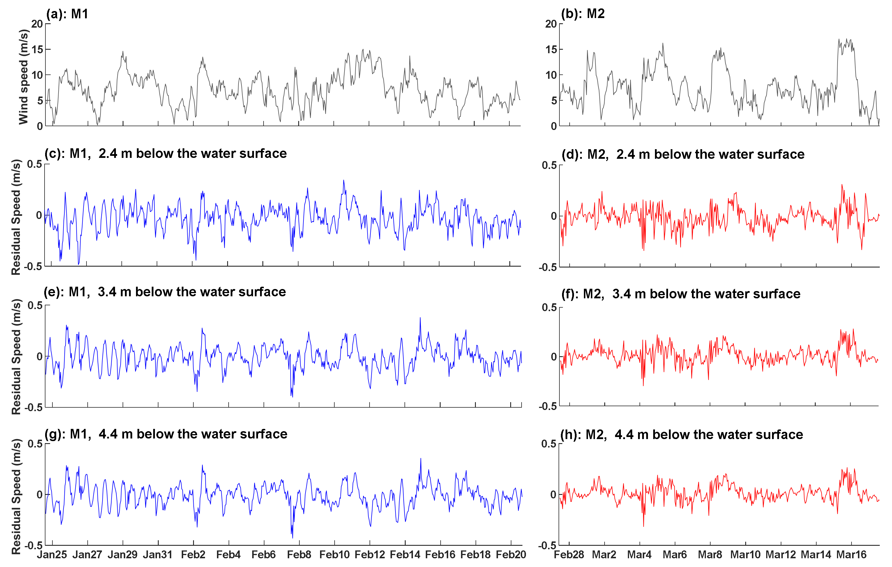
3.2.4. Residual Current and Wind Speed

The residual current time series of each layer in Figure 6 was obtained through harmonic analysis. At the M1 station, the average values of the residual current at 2.4 m (Figure 6c), 3.4 m (Figure 6e), and 4.4 m (Figure 6g) underwater were 0.102 m/s, 0.090 m/s, and 0.087 m/s, respectively, indicating that the closer to the water surface, the greater the residual current. As demonstrated by Figure 6a, the increase or decrease in wind speed has a small effect on the changes in the residual current in the upper layer at M1 station, and the correlation analysis results showed that the wind speed was not related to the residual current in each layer at M1 station. At M2 station, the average values of the residual current at 2.4 m (Figure 6d), 3.4 m (Figure 6f), and 4.4 m (Figure 6h) underwater were 0.078 m/s, 0.064 m/s, and 0.059 m/s, respectively, also indicating that the closer to the water surface, the greater the residual current. As shown in Figure 6b, the change in the residual current in the upper layer of M2 was significantly affected by the increase or decrease in wind speed. The correlation analysis results revealed that there was a significant positive correlation between the wind speed and residual current at 2.4 m, 3.4 m, and 4.4 m underwater at the M2 station, with correlation coefficients of 0.10, 0.41, and 0.43, respectively, which passed the 95%, 99%, and 99% confidence tests. Correlation analysis suggested that when there was no sea ice cover, wind speed had a strong control effect on the residual current; when there was sea ice cover, the sea ice partially shielded the effect of wind speed on the residual current, greatly weakening the controlling action of the wind field.

3.3. Impact of Sea Ice on Suspended Sediment Concentration

3.3.1. Vertical Profile of Backscatter Intensity at Full Water Depth

Figure 7b,d shows that the backscatter intensity at the bottom layer of the M1 station was significantly lower than that of the M2 station and exhibited stronger pulsation, whereas the backscatter intensity at the bottom layer of M2 was generally higher and the changes were relatively continuous. The variations of backscatter intensity at the M1 station were mainly controlled by the spring–neap tidal cycle (namely, the change of SSC was mainly controlled by the spring–neap tidal cycle). For instance, during the spring tide on February 2–4 and February 14–16, the backscatter intensity was high; during the neap tide on January 28 and February 12, the backscatter intensity was low. However, the period of February 7–8 was an exception. Although this period was a neap tide period, the backscatter intensity suddenly increased. As shown by the residual current data at M1 in Figure 6e,g, there was a maximum residual current up to 0.4 m/s during this period, which may be the reason for the sudden increase in backscatter intensity during this period. The backscatter intensity at the bottom of the M2 station indicated that turbulent resuspension events occurred on March 4 and March 15, and the backscatter intensity fluctuated in high frequency. The resuspension events were caused by the high TKE induced by strong winds greater than 15 m/s on March 4 and 15. Consequently, the variation of the backscatter intensity at the M2 station was mainly controlled by the wind field; namely, the variation of SSC was mainly controlled by the wind field. The impact mechanism will be discussed in further detail in the Discussion section.
Figure 7a,c indicated that the change in backscatter intensity in the middle and upper layers of water bodies at M1 and M2 was the upward diffusion of the change at the bottom layer. The M1 station was mainly controlled by the spring–neap tidal cycles, whereas the M2 station was mainly affected by the wind field. The backscatter intensity of the middle and upper water bodies at the M2 station ranged from 100 to 145, whereas that at the M1 station ranged from 90 to 130; the latter was obviously smaller than the former, indicating that the SSC in water bodies covered by sea ice was significantly lower.

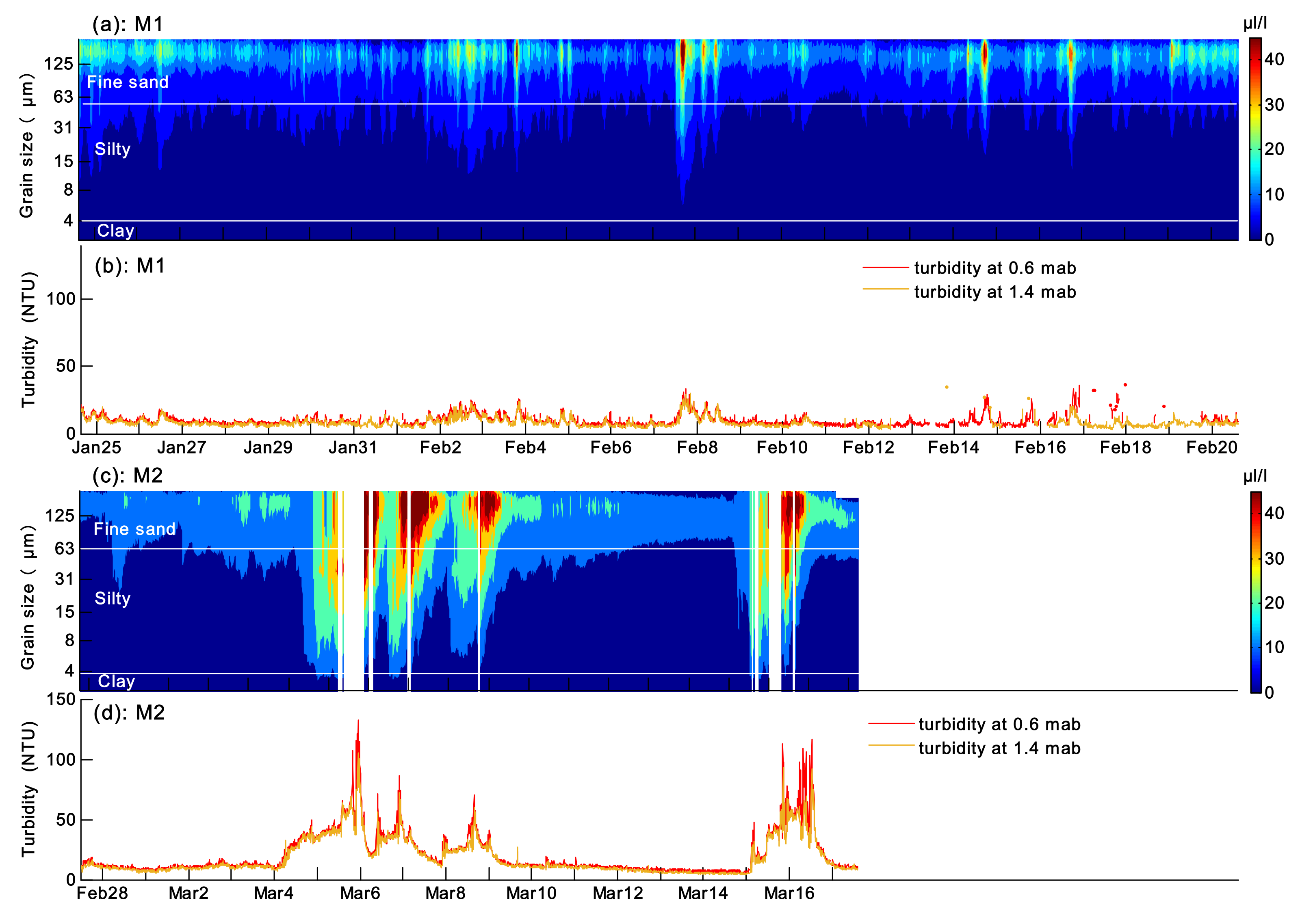
3.3.2. Volume Concentration, Particle Size Distribution, and Turbidity of Suspended Sediment at the Bottom Layer

The volume concentration of suspended sediment observed by the LISST in Figure 8a,c indicated that the red high-value area of volume concentration at the M1 station was less apparent with a very short coverage period, whereas that at the M2 station was more apparent with a longer coverage period. Moreover, the statistical results showed that the average volume concentration at the M1 station during the observation period was 4.9 μL/L, whereas that at the M2 station was 9.3 μL/L, indicating that the volume concentration at the bottom of the M1 station with sea ice cover was smaller, which was approximately half of the concentration at the M2 station without sea ice cover.
The analysis results of the sampled seabed sediment at the two stations are described as follows. The seabed sediment diameters at 90%, 50%, and 10% of the cumulative curve at M1 station were 203 μm (fine sand), 17 μm (silt), and 2 μm (clay), respectively; and those at M2 station were 282 μm (medium sand), 157 μm (fine sand), and 4 μm (clay), respectively. The LISST results showed that the suspended sediment at M1 mainly comprised fine sand, followed by silt, with scarcely any clay. The average volume concentrations of these three particle sizes during the observation period were 11.4 μL/L, 3 μL/L, and 0.2 μL/L, respectively, accounting for 78%, 21%, and 1% of the total, respectively. The suspended sediment at M2 mainly comprised fine sand, followed by silt and finally clay. The average volume concentrations of these three particle sizes were 18.4 μL/L, 7.9 μL/L, and 1.6 μL/L, respectively, accounting for 66%, 28%, and 6% of the total, respectively. The grain size of the seabed sediment comprising fine sand and silt at M1 was relatively small. Under the conditions of sea ice cover, there were fewer suspended particles, which were mainly non-cohesive fine sand, accounting for 78% of the total. The grain size of the seabed sediment mainly composed of medium sand and fine sand at M2 was relatively large, but there were more suspended particles, including 34% cohesive particles in addition to 66% non-cohesive fine sand. This indicated that the particle size component most likely to resuspend in this area was fine sand. Even with sea ice cover and weak hydrodynamic conditions, fine sand would resuspend slightly (M1), whereas cohesive particles would only resuspend under strong hydrodynamic conditions (M2).
It can be observed from Figure 8a–d that the variations in volume concentration and turbidity of suspended sediment at the bottom of the two stations corresponded with each other, with the same occurrence time for high values. Figure 8b,d demonstrated that the turbidity at 0.6 mab and 1.4 mab showed the same trend, the turbidity at 0.6 mab was slightly higher than that at 1.4 mab, and the average turbidity at M1 was lower than that at M2. Throughout the observation period, the turbidity of M1 was at a low level and the change was relatively smooth, with an average of 8.6 NTU and a highest value of 36 NTU (February 16). The turbidity of M2 remained low when the wind speed was small, increased sharply by three times under the influence of 4 gales at 15 m/s or above (except March 1), with the highest value being up to 132.6 NTU (March 5) and with an average turbidity of 17.8 NTU throughout the observation period.
According to the distribution of surface SSC in the Bohai Sea (Figure 1), it can be observed that M1 was located in the region with higher multi-year average SSC (30–100 mg/L), which was higher than that of M2 in the region with lower multi-year average SSC (10–30 mg/L). Nevertheless, under the impact of sea ice, the near-bottom volume concentration and turbidity of M1 were lower than the multi-year average values, resulting in a reversal of low SSC at M1 but high SSC at M2.

4. Discussion

4.1. Causes of Low SSC under the Impact of Sea Ice

The analysis of the backscatter intensity in Section 3.3.1 indicated that the change in SSC at M2 without sea ice cover was controlled by the wind field, the SSC was high, and resuspension occurred twice when the wind speed was higher than 15 m/s. However, at the M1 station, the wind field was shielded when sea ice was covered, and the resuspension was mainly controlled by the spring–neap tidal cycle, and the SSC was low. The differences in hydrodynamic conditions at the two stations caused the differences in SSC.
The strength of hydrodynamic conditions can be represented by TKE, as shown in Figure 9. The near-bottom TKEs at the two stations were compared, and the correlation between the wind speed and the near-bottom TKE at the two stations was analyzed. As shown in Figure 9, the near-bottom TKE at M1 remained low throughout the observation period, with an average of 0.3 m2/s2 and a maximum of 6.6 m2/s2; the near-bottom TKE at station M2 was relatively high, with an average of 0.9 m2/s2, while the peak TKE corresponded to the high wind speed. For example, the peak TKE of 19.8 m2/s2 at 11:00 on March 4 corresponded to the strong wind on March 4. Correlation analysis showed that the wind speed at M1 was not correlated with the near-bottom TKE; furthermore, the correlation coefficient between the wind speed and the near-bottom TKE at M2 was 0.30, which was a significant positive correlation (passing the 99% confidence test). This indicated that the strong wind at M1 was shielded by the ice surface and could not disturb the hydrodynamic environment dominated by the tide below the ice surface. Hence, the near-bottom TKE remained low, and the near-bottom water body was stable, which could not induce the turbulent resuspension of the sediment; thus, the SSC in the water body remained low.
In addition, the strength and duration of the sediment resuspension mainly depend on the bottom shear stress. When the bottom shear stress is large, the sediment resuspension is intense and the duration is long. The bottom shear stress was mainly tide-induced shear stress at the M1 station, which was only controlled by the spring–neap tidal cycle under ice shielding. At the M2 station, under the control of the wind field, the bottom shear stress included wave-induced shear stress in addition to the tide-induced shear stress; furthermore, the wave-induced shear stress could be an order of magnitude larger than the tide-induced shear stress under strong wind conditions [50,51,52], thus playing a dominant role. Consequently, at the M1 station, owing to the presence of ice, the wave-induced shear stress inducing strong resuspension was shielded, resulting in low resuspension strength and low SSC.

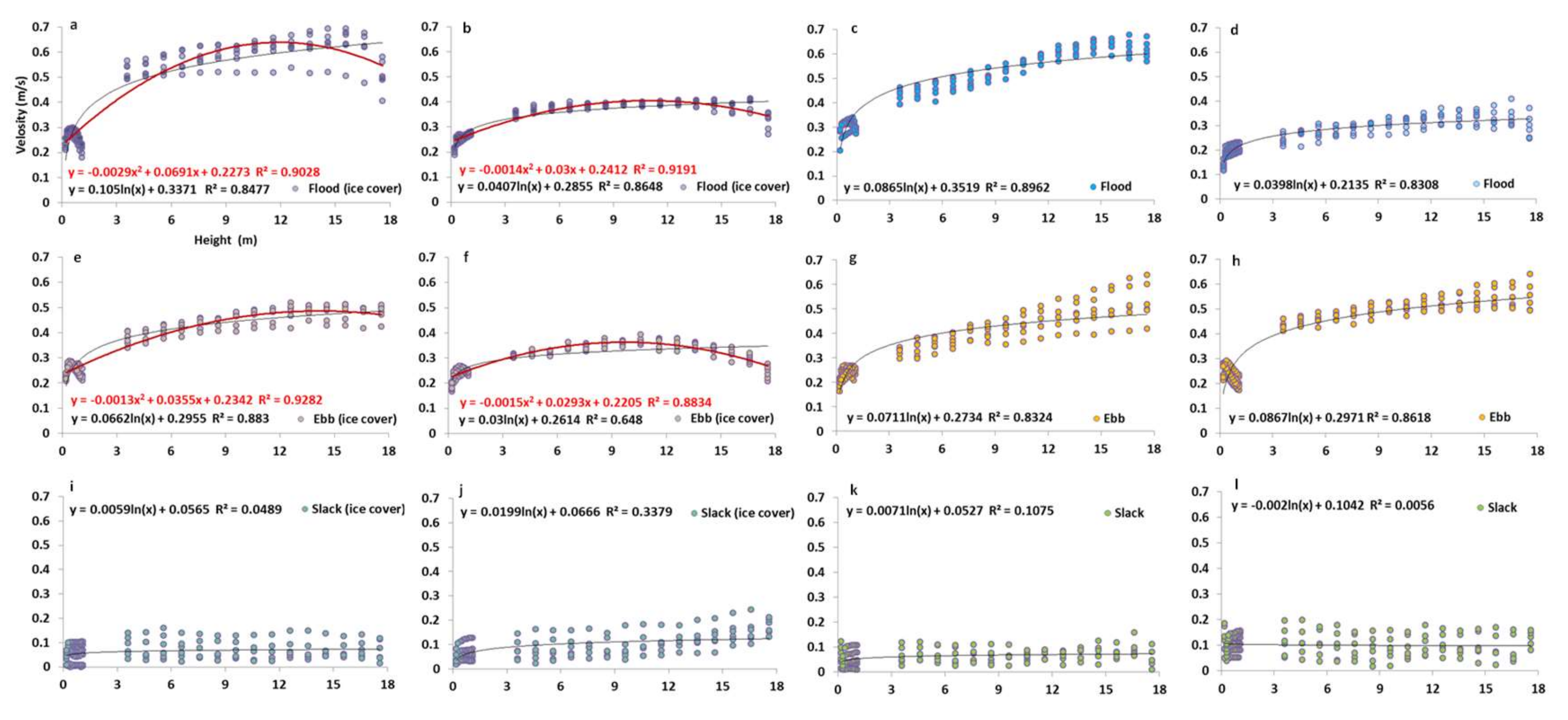
4.2. Vertical Distribution of Velocity and SSC with or without Sea Ice

To explore the similarities and differences in vertical distribution of velocity and SSC in different tidal phases during typical spring tide periods with or without sea ice, we first selected typical spring tide periods based on the changes in tidal current velocity at M1, along with the envelope curve (Figure 5c). These periods were February 2, 3, and 4 (with ice cover), and February 17, 18, and 19 (without ice cover). We then performed regression analysis between the velocity and the height from the bottom, as well as between the backscatter intensity and the height from the bottom, in different tidal phases during these typical spring tide periods (high tide, ebb tide, and slack water). Then, we obtained the scatter plots and fitting relations of the current velocity (Figure 10) and of the backscatter intensity at different heights from the bottom (Figure 11).
Under ice-free conditions, the upper current velocity during the flood and ebb tide periods mainly increased with the height from the bottom. As shown in Figure 10c,d,g,h, the vertical distribution was logarithmic, and the logarithmic fitting coefficient R2 was above 0.83. Under ice-covered conditions, as shown in Figure 10a,b,e,f, the upper current velocity displayed a significant downward trend during the periods of flood tide and ebb tide; that is, the velocity of several layers near the sea surface was smaller than that of the lower layer. Such a significant downward trend of current velocity was most typical in the ebb velocity distribution, shown in Figure 10f. The logarithmic fitting coefficient of the vertical velocity was only 0.648, whereas the parabolic fitting coefficient reached 0.88. Other parabolic fitting of the current velocity distribution of flood and ebb tides (Figure 10a,b,e) under sea ice cover conditions showed that the fitting coefficient values were significantly increased (all were above 0.90) compared with those of the logarithmic fitting, indicating that the vertical velocity distribution under the sea ice cover was no longer logarithmic but was parabolic [1]. This was because the solid ice boundary instead of the air–sea interface increased the drag coefficient of the surface water body and suppressed the flow of the upper layer seawater to a certain extent, so that the upper layer velocity no longer increased but decreased with the increase in height from the bottom.
As shown in Figure 10i–l, the vertical logarithmic distribution of velocity was not evident during the slack water period, and the vertical structure with ice cover was almost the same as the vertical structure without ice cover. This was because during the slack water period, the flow of the entire water body was very stable, with a small current velocity for each layer and small vertical changes, and the suppression effect of the ice sheet did not affect the vertical velocity structure of the water body in this steady state.
In addition to discussing the typical tidal phases, we further statistically clarified the impact of sea ice cover on the vertical distribution of velocity and calculated the distribution percentages of the maximum velocity in each water layer at M1 and M2 stations. During the sea ice cover period at M1 station, the percentages of the maximum vertical velocity appearing in the upper six layers near the water surface from top to bottom were 24% (2.4 m underwater), 36% (3.4 m underwater), 19% (4.4 m underwater), 9% (5.4 m underwater), 8% (6.4 m underwater), and 4% (7.4 m underwater). During the observation period at M2 station, the percentages of the maximum vertical velocity appearing in the upper six layers near the water surface from top to bottom were 56% (2.4 m underwater), 22% (3.4 m underwater), 7% (4.4 m underwater), 6% (5.4 m underwater), 5% (6.4 m underwater), and 4% (7.4 m underwater). It can be observed from the percentage distribution of the maximum velocity in the upper layer that when there was sea ice cover, only a small part (24%) of the maximum velocity was distributed in the uppermost layer (the 2.4 m layer underwater) of the observed velocity with the majority distributed in the 3.4 m layer underwater (36%). When there was no sea ice cover, more than half of the maximum velocity was distributed in the uppermost layer—the 2.4 m layer underwater—and the percentage of the maximum value in the stream layer decreased sharply with increasing depth.
It can be observed from Figure 11 that under conditions with or without sea ice cover, the vertical distribution structure of the backscatter intensity in each tidal phase period was consistent. The backscatter intensity near the bottom (0.16–1.5 mab) in each tidal phase period was higher, and its vertical gradient was also larger; as the height from the bottom increased (above 3 mab), the backscatter intensity gradually decreased, and the overall distribution was logarithmic. This showed that the vertical distribution of SSC in each tidal phase with sea ice cover was almost the same as that without sea ice cover, and that sea ice did not affect the vertical distribution of SSC. There may be two reasons for this phenomenon: one was that the SSC in the observation area was low and varied little with time; the other was that the sea ice in the observation area was thin (approximately 10 cm in thickness), which had limited impact on the hydrodynamic environment, especially the above-mentioned vertical distribution of velocity, and therefore could not change the vertical distribution structure of the SSC.

5. Conclusions

Based on the 45-day synchronous observation data of full-water-depth flow and sediment at the two stations (with ice at M1 station and without ice at M2 station) in the Qinhuangdao waters in the Bohai Sea in the winter of 2018, the quantitative impacts of sea ice on the hydrodynamic conditions, sediment resuspension, and suspended sediment distribution in the study area were analyzed systematically.
The seawater icing event on January 28 reduced the water temperature at the bottom layer by 1.77 °C within 4 h, while increasing the salinity at the bottom layer by 0.4 psu due to brine rejection during the process of seawater freezing.
The main velocity component was the periodic tidal current, and the residual current was generally less than 0.1 m/s. As the M2 station was closer to the amphidromic point of the Bohai Sea, the velocity of the ice-covered M1 station was still greater than that of the M2 station as a whole. Owing to the shielding effect of sea ice, the variation of the residual current was hardly affected by the change of the wind field.
During the period of sea ice coverage, the average volume concentration of the suspended sediment at the bottom layer was 4.9 μL/L and the average turbidity was 8.6 NTU, which were only approximately half of the values without sea ice cover, namely 9.3 μL/L and 17.8 NTU, respectively. The grain size component most prone to resuspension in this sea area was fine sand, and the resuspension of cohesive sediment could occur under strong hydrodynamic conditions alone.
The suppression of sea ice maintained a low near-bottom TKE, with an average of 0.3 m2/s2 and a maximum of merely 6.6 m2/s2, which had no response to strong winter monsoon winds greater than 15 m/s. The low TKE implied that the near-bottom water body was stable and could not induce turbulent resuspension, and the SSC in the water body remained low. When there was no sea ice cover, strong wind forcing in winter could generate high TKE, with a maximum of 19.8 m2/s2, thus inducing turbulent resuspension events; thereafter, the sediment resuspension dominated by wave-induced shear stress continued to occur, leading to a continuous increase in SSC.
Under the condition of sea ice cover, the boundary of the solid ice surface increased the drag coefficient of the surface water body, which suppressed the flow of the upper seawater. When the current velocity was high during the flood and ebb tides, the vertical distribution of current velocity was no longer a traditional logarithmic type but was parabolic. Matched with the parabolic vertical velocity distribution, when the ice cover was approximately 10 cm thick, the maximum vertical velocity was mainly distributed in the 3.4 m layer underwater. During the period of sea ice cover, the SSC was low and the ice layer was thin; hence, the existence of sea ice did not affect the vertical distribution of SSC in the water body.

Author Contributions

Conceptualization, C.P. and M.J.; methodology, C.P. and M.J.; software, M.J.; validation, C.P.; formal analysis, C.P. and M.J.; investigation, Z.L. and J.J.; resources, C.P.; data curation, C.P. and M.J.; writing—original draft preparation, M.J.; writing—review and editing, C.P.; visualization, M.J.; supervision, C.P.; project administration, C.P.; funding acquisition, C.P. All authors have read and agreed to the published version of the manuscript.

Funding

This research was funded by the National Natural Science Foundation of China (Grant No. 41576060), Joint Fund between Natural Science Foundation of China and Shandong Province (Grant No. U1406401), the National Key R&D Program of China (Grant No. 2016YFC0301203), Research Foundation for Advanced Talent (Grant No. 2019YB020), and Hebei Science and Technology Project (Grant No.19273301D).

Acknowledgments

The authors thank all of the investigators for their help in collecting samples and data during the field survey.

Conflicts of Interest

The authors declare no conflict of interest.

References

  1. McGraw, M.C.; Barnes, E.A. New Insights on Subseasonal Arctic-Midlatitude Causal Connections from a Regularized Regression Model. J. Clim. 2020, 33, 213–228. [Google Scholar] [CrossRef]
  2. Ayarzagüena, B.; Screen, J.A. Future Arctic sea ice loss reduces severity of cold air outbreaks in midlatitudes. Geophys. Res. Lett. 2016, 43, 2801–2809. [Google Scholar] [CrossRef]
  3. Francis, J.A. The Arctic matters: Extreme weather responds to diminished Arctic Sea ice. Environ. Res. Lett. 2015, 10, 091002. [Google Scholar] [CrossRef]
  4. Petoukhov, V.; Semenov, V.A. A link between reduced Barents-Kara sea ice and cold winter extremes over northern continents. J. Geophys. Res. 2010, 115, D21111. [Google Scholar] [CrossRef]
  5. Parkinson, C.L.; Cavalieri, D.J.; Gloersen, P.; Zwally, H.J.; Comiso, J.C. Arctic sea ice extents, areas, and trends, 1978–1996. J. Geophys. Res. Oceans 1999, 104, 20837–20856. [Google Scholar] [CrossRef]
  6. Overpeck, J. Arctic Environmental Change of the Last Four Centuries. Science 1997, 278, 1251–1256. [Google Scholar] [CrossRef] [Green Version]
  7. Liu, W.; Fedorov, A.; Sévellec, F. The mechanisms of the Atlantic Meridional Overturning Circulation slowdown induced by Arctic sea ice decline. J. Clim. 2019, 32, 977–996. [Google Scholar] [CrossRef]
  8. Liu, W.; Fedorov, A.V. Timescales and mechanisms of global climate impacts of Arctic sea ice loss mediated by the Atlantic meridional overturning circulation. Geophys. Res. Lett. 2019, 46, 944–952. [Google Scholar] [CrossRef]
  9. Stein, R. The late Mesozoic—Cenozoic Arctic Ocean climate and sea ice history: A challenge for past and future scientific ocean drilling. Paleoceanogr. Paleoclimatol. 2019, 34, 1851–1894. [Google Scholar] [CrossRef] [Green Version]
  10. Kern, S.; Lavergne, T.; Notz, D.; Pedersen, L.T.; Tonboe, R.T.; Saldo, R.; Sørensen, A.M. Satellite passive microwave sea ice concentration data set intercomparison: Closed ice and ship-based observations. Cryosphere Copernic. Publ. 2019, 13, 3261–3307. [Google Scholar] [CrossRef] [Green Version]
  11. Screen, J.A.; Simmonds, I. The central role of diminishing sea ice in recent Arctic temperature amplification. Nature 2010, 464, 1334–1337. [Google Scholar] [CrossRef] [PubMed] [Green Version]
  12. Comiso, J.C.; Parkinson, C.L.; Gersten, R.; Stock, L. Accelerated decline in the Arctic sea ice cover. Geophys. Res. Lett. 2008, 35, L01703. [Google Scholar] [CrossRef] [Green Version]
  13. Jiao, C.; Zhang, W.; Dong, S. Statistical Prediction for Annual Start Date and Duration of Sea ice Coverage at Qinhuangdao Observation Station. J. Ocean Univ. Chin. 2019, 18, 1265–1272. [Google Scholar] [CrossRef]
  14. Manson, G.K.; Davidson-Arnott, R.G.D.; Ollerhead, J. Attenuation of Wave Energy by Nearshore Sea Ice: Prince Edward Island, Canada. J. Coastal Res. 2016, 318, 253–263. [Google Scholar]
  15. Kug, J.-S.; Jeong, J.-H.; Jang, Y.-S.; Kim, B.-M.; Folland, C.K.; Min, S.-K.; Son, S.-W. Two distinct influences of Arctic warming on cold winters over North America and East Asia. Nat. Geosci. 2015, 8, 759–762. [Google Scholar] [CrossRef]
  16. Grebmeier, J.; Frey, K.; Cooper, L.; Kędra, M. Trends in Benthic Macrofaunal Populations, Seasonal Sea Ice Persistence, and Bottom Water Temperatures in the Bering Strait Region. Oceanography 2018, 31, 136–151. [Google Scholar] [CrossRef] [Green Version]
  17. Wegner, C.; Wittbrodt, K.; Hölemann, J.A.; Janout, M.A.; Krumpen, T.; Selyuzhenok, V.; Timokhov, L. Sediment entrainment into sea ice and transport in the Transpolar Drift: A case study from the Laptev Sea in winter 2011/2012. Cont. Shelf Res. 2017, 141, 1–10. [Google Scholar] [CrossRef] [Green Version]
  18. Forest, A.; Osborne, P.D.; Curtiss, G.; Lowings, M.G. Current surges and seabed erosion near the shelf break in the Canadian Beaufort Sea: A response to wind and ice motion stress. J. Mar. Syst. 2016, 160, 1–16. [Google Scholar] [CrossRef]
  19. Sanchez-Vidal, A.; Veres, O.; Langone, L.; Ferré, B.; Calafat, A.; Canals, M.; Danovaro, R. Particle sources and downward fluxes in the eastern Fram strait under the influence of the west Spitsbergen current. Deep Sea Res. Part I 2015, 103, 49–63. [Google Scholar] [CrossRef] [Green Version]
  20. Eicken, H.; Gradinger, R.; Gaylord, A.; Mahoney, A.; Rigor, I.; Melling, H. Sediment transport by sea ice in the Chukchi and Beaufort Seas: Increasing importance due to changing ice conditions? Deep Sea Res. Part II 2005, 52, 3281–3302. [Google Scholar] [CrossRef]
  21. Boone, W.; Rysgaard, S.; Kirillov, S.; Dmitrenko, I.; Bendtsen, J.; Mortensen, J.; Barber, D.G. Circulation and fjord-shelf exchange during the ice-covered period in Young Sound-Tyrolerfjord, Northeast Greenland (74° N). Estuar. Coast. Shelf Sci. 2017, 194, 205–216. [Google Scholar] [CrossRef]
  22. Miller, M.F.; Fan, Z.; Bowser, S.S. Sediments Beneath Multi-Year Sea Ice: Delivery By Deltaic and Eolian Processes. J. Sediment. Res. 2015, 85, 301–314. [Google Scholar] [CrossRef]
  23. Murray, K.T.; Miller, M.F.; Bowser, S.S. Depositional processes beneath coastal multi-year sea ice. Sedimentology 2012, 60, 391–410. [Google Scholar] [CrossRef]
  24. Walker, T.R.; Grant, J.; Cranford, P.; Lintern, D.G.; Hill, P.; Jarvis, P.; Nozais, C. Suspended sediment and erosion dynamics in Kugmallit Bay and Beaufort Sea during ice-free conditions. J. Mar. Syst. 2008, 74, 794–809. [Google Scholar] [CrossRef]
  25. Drews, C. Using Wind Setdown and Storm Surge on Lake Erie to Calibrate the Air-Sea Drag Coefficient. PLoS ONE 2013, 8, e72510. [Google Scholar] [CrossRef]
  26. Peck, L.S.; Barnes, D.K.A.; Willmott, J. Responses to extreme seasonality in food supply: Diet plasticity in Antarctic brachiopods. Mar. Biol. 2005, 147, 453–463. [Google Scholar] [CrossRef]
  27. Giesbrecht, T.; Sim, N.; Orians, K.J.; Cullen, J.T. The distribution of dissolved and total dissolvable aluminum in the Beaufort Sea and Canada Basin region of the Arctic Ocean. J. Geophys. Res. Oceans. 2013, 118, 6824–6837. [Google Scholar] [CrossRef]
  28. Bonsell, C.; Dunton, K.H. Long-term patterns of benthic irradiance and kelp production in the central Beaufort sea reveal implications of warming for Arctic inner shelves. Prog. Oceanogr. 2018, 162, 160–170. [Google Scholar] [CrossRef]
  29. Lannuzel, D.; Schoemann, V.; de Jong, J.; Pasquer, B.; van der Merwe, P.; Masson, F.; Bowie, A. Distribution of dissolved iron in Antarctic sea ice: Spatial, seasonal, and inter-annual variability. J. Geophys. Res. 2010, 115, G03022. [Google Scholar] [CrossRef]
  30. Forest, A.; Sampei, M.; Makabe, R.; Sasaki, H.; Barber, D.G.; Gratton, Y.; Fortier, L. The annual cycle of particulate organic carbon export in Franklin Bay (Canadian Arctic): Environmental control and food web implications. J. Geophys. Res. 2008, 113, C03S05. [Google Scholar]
  31. Pang, C.G.; Yu, W. Spatial modes of suspended sediment concentration in surface water in Bohai Sea and their temporal variations. Adv. Water Sci. 2013, 24, 722–727, (in Chinese with English abstract). [Google Scholar]
  32. Yuan, D.L.; Zhu, J.R.; Li, C.Y.; Hu, D.X. Cross-shelf circulation in the Yellow and East China Seas indicated by MODIS satellite observations. J. Mar. Syst. 2008, 70, 134–149. [Google Scholar] [CrossRef]
  33. National Marine Environmental Forecasting Center. Available online: http://www.nmefc.cn/haibing/jingbaodetail.aspx (accessed on 16 February 2020).
  34. RD Instruments. Principles of Operation A Practical Primer; RD Instruments: San Diego, CA, USA, 1996; pp. 38–39. [Google Scholar]
  35. Lan, Z.G.; Gong, D.J.; Yu, X.S.; Li, S.R.; Xu, Y.P. Particle size correction of suspended sediment concentration measured by ADCP with in-situ particle size analyzer. Oceanol. Limnol. Sin. 2004, 35, 385–392, (in Chinese with English abstract). [Google Scholar]
  36. Deines, K.L. Backscatter estimation using broadband acoustic Doppler Current Profilers. In Proceedings of the IEEE Sixth Working Conference on Current Measurement, San Diego, CA, USA, 13 March 1999; pp. 249–253. [Google Scholar]
  37. Soulsby, R.L.; Dyer, K.R. The form of the near-bed velocity profile in a tidally accelerating flow. J. Geophys. Res. 1981, 86, 8067. [Google Scholar] [CrossRef]
  38. Stapleton, K.R.; Huntley, D.A. Seabed stress determinations using the inertial dissipation method and the turbulent kinetic energy method. Earth Surf. Process. Landforms. 1995, 20, 807–815. [Google Scholar] [CrossRef]
  39. Kim, S.-C.; Friedrichs, C.T.; Maa, J.P.-Y.; Wright, L.D. Estimating Bottom Stress in Tidal Boundary Layer from Acoustic Doppler Velocimeter Data. J. Hydraul. Eng. 2000, 126, 399–406. [Google Scholar] [CrossRef] [Green Version]
  40. Zhu, Q.; van Prooijen, B.C.; Wang, Z.B.; Ma, Y.X.; Yang, S.L. Bed shear stress estimation on an open intertidal flat using in situ measurements. Estuar. Coast. Shelf Sci. 2016, 182, 190–201. [Google Scholar] [CrossRef]
  41. Yuan, Y. Observations of Suspended Sediment Dynamics in Chinese Coastal Seas by Acoustic Instruments. PhD Thesis, Ocean University of China, Qingdao, China, 5 June 2009. [Google Scholar]
  42. Stacey, M.T.; Monismith, S.G.; Burau, J.R. Measurements of Reynolds stress profiles in unstratified tidal flow. J. Geophys. Res. Oceans 1999, 104, 10933–10949. [Google Scholar] [CrossRef]
  43. Bian, C.; Liu, Z.; Huang, Y.; Zhao, L.; Jiang, W. On estimating turbulent Reynolds stress in wavy aquatic environment. J. Geophys. Res. Oceans 2018, 123, 3060–3071. [Google Scholar] [CrossRef]
  44. MacVean, L.J.; Lacy, J.R. Interactions between waves, sediment, and turbulence on a shallow estuarine mudflat. J. Geophys. Res. Oceans 2014, 119, 1534–1553. [Google Scholar] [CrossRef]
  45. Kularatne, S.; Pattiaratchi, C. Turbulent kinetic energy and sediment resuspension due to wave groups. Cont. Shelf Res. 2008, 28, 726–736. [Google Scholar] [CrossRef] [Green Version]
  46. Wright, L.; Xu, J.; Madsen, O. Across-shelf benthic transports on the inner shelf of the Middle Atlantic Bight during the “Halloween storm” of 1991. Mar. Geol. 1994, 118, 61–77. [Google Scholar] [CrossRef]
  47. Soulsby, R. Dynamics of Marine Sands: A Manual for Practical Applications; Tomas Telford Limited: London, UK, 1997; pp. 72–76. [Google Scholar]
  48. Hou, Q.Z.; Lu, Y.J.; Wang, Z.L. Cumulative impacts of high intensity reclamation in Bohai Bay on tidal wave system and its mechanism. Chin. Sci. Bull. 2017, 62, 3479–3489. [Google Scholar] [CrossRef]
  49. Huang, J.; Xu, J.; Gao, S.; Lian, X.; Li, J. Analysis of Influence on the Bohai Sea Tidal System Induced by Coastline Modification. J. Coastal Res. 2015, 73, 359–363. [Google Scholar] [CrossRef]
  50. Chang, G.C.; Dickey, T.D.; Williams, A.J. Sediment resuspension over a continental shelf during Hurricanes Edouard and Hortense. J. Geophys. Res. Oceans. 2001, 106, 9517–9531. [Google Scholar] [CrossRef]
  51. Glenn, S.M.; Grant, W.D. A suspended sediment stratification correction for combined wave and current flows. J. Geophys. Res. 1987, 92, 8244–8264. [Google Scholar] [CrossRef]
  52. Dufois, F.; Garreau, P.; Le Hir, P.; Forget, P. Wave- and current-induced bottom shear stress distribution in the Gulf of Lions. Cont. Shelf Res. 2008, 28, 1920–1934. [Google Scholar] [CrossRef] [Green Version]
Figure 1. The position of Bohai Sea and its distribution of average surface suspended sediment concentration in winter, as well as sea ice information. (a) Distribution of average surface suspended sediment concentration in winter in the Bohai Sea in 1998–2004 retrieved from ocean color remote sensing inversion [31]. The red circles are the in situ observation stations for flow and sediment, which are stations M1 and M2, respectively. The blue circles are the offshore buoys used to measure sea surface wind speed. (b) The position of the Bohai Sea [32]. (c,d) Sea ice images of the study area on 29 January 2018 and 5 February 2018, respectively, contain the ice cover area and ice thickness information, which were downloaded from the National Marine Environmental Forecasting Center [33].
Water 12 00611 g001
Figure 2. Seabed observation platform. Note: ADV, acoustic Doppler velocimeter, ADCP, acoustic Doppler current profiler; PC-ADP, pulse-coherent acoustic Doppler profiler; LISST, laser in situ scattering and transmissometry; OBS, optical backscatter sensor; CTD, conductivity temperature depth sensor.
Water 12 00611 g002
Figure 3. Changes in wind speed (a,b), temperature (c,d), salinity (e,f), and water depth (g,h) at stations M1 and M2.
Water 12 00611 g003
Figure 4. Original velocity profile at full water depth measured by upward-looking ADCP and downward-looking PCADP. (a) Vertical profile of current velocity in the middle and upper layers of the water body at M1 station, measured by upward-looking ADCP. (b) Vertical profile of current velocity in the near bottom layers of the water body at M1 station, measured by downward-looking PCADP. (c) Vertical profile of current velocity in the middle and upper layers of the water body at M2 station, measured by upward-looking ADCP. (d) Vertical profile of current velocity in the near bottom layers of the water body at M2 station, measured by downward-looking PCADP.
Water 12 00611 g004
Figure 5. (a,b) Demonstration of MATLAB t_tide toolbox analysis for M1 (16.6 mab) and M2 (14.6 mab), respectively. (c,d) Tidal currents from t_tide analysis. (e,f) Analyzed lines with 95% significance levels for M1 and M2, respectively. (g,h) Spectral estimates before and after the removal of tidal energy for M1 and M2, respectively.
Water 12 00611 g005
Figure 6. Variation in wind speed and upper residual current at M1 and M2 stations. (a,b) Wind speeds at M1 and M2 stations, respectively. (c,d) Residual currents at 2.4 m at M1 and M2 stations, respectively. (e,f) Residual currents at 3.4 m at M1 and M2 stations, respectively. (g,h) Residual currents at 4.4 m at M1 and M2 stations, respectively.
Water 12 00611 g006
Figure 7. Vertical profile of backscatter intensity at full water depth, estimated by the echo intensity measured by the upward-looking ADCP (a,c) and downward-looking PCADP (b,d).
Water 12 00611 g007
Figure 8. Volume concentration, particle size distribution (a,c), and water turbidity (b,d) at the bottom layer at M1 and M2 stations, respectively, measured by LISST (a,c) and OBS (b,d).
Water 12 00611 g008
Figure 9. Comparison of wind speed and near-bottom turbulent kinetic energy (TKE) at M1 and M2 stations, respectively.
Water 12 00611 g009
Figure 10. Scatter plots and fitting relations of current velocity at different heights from the bottom in different tidal phases during typical spring tide periods: (a,b) the periods of flood tide with ice cover on February 2 and 3; (c,d) the periods of flood tide without ice cover on February 17 and 18; (e,f) the periods of ebb tide with ice cover on February 3 and 4; (g,h) the periods of ebb tide without ice cover on February 18 and 19; (i,j) two periods of slack water with ice cover on February 3; (k,l) two periods of slack water without ice cover on February 18.
Water 12 00611 g010
Figure 11. Scatter plots and fitting relations of current velocity at different heights from the bottom in different tidal phases during typical spring tide periods: (a) the flood tide period with ice cover on February 2; (b) the ebb tide period with ice cover on February 2; (c) the slack water period with ice cover on February 3; (d) the flood tide period without ice cover on February 17; (e) the ebb tide period without ice cover on February 18; (f) the slack water period without ice cover on February 18.
Water 12 00611 g011
Table 1. Overview of instrument configuration.
ObservationInstrumentHeight (mab 1)Sampling Interval
Current velocity and echoADCP210 min
Current velocity and echoPC-ADP1.5510 min
High frequency velocityADV0.820 min (M1); 10 min (M2)
SSC (volume) and grain sizeLISST1.830 min
TurbidityOBS1.4/0.610 min
Temperature, salinity, and depthCTD1.810 min
Note: 1 mab, meters above the bed; SSC, suspended sediment concentration.

