1. Introduction
As the country with the richest hydropower potential in the world, China has made tremendous achievements in hydropower industry development during the past two decades [
1]. By the end of 2019, China’s installed hydropower generation capacity reached 356.4 GW [
2] (18% of its total installed generation capacity), ranking first in the world. Affected by rainfall, the distribution of hydropower resources in China is uneven. A majority of hydropower bases are located in the southwest regions [
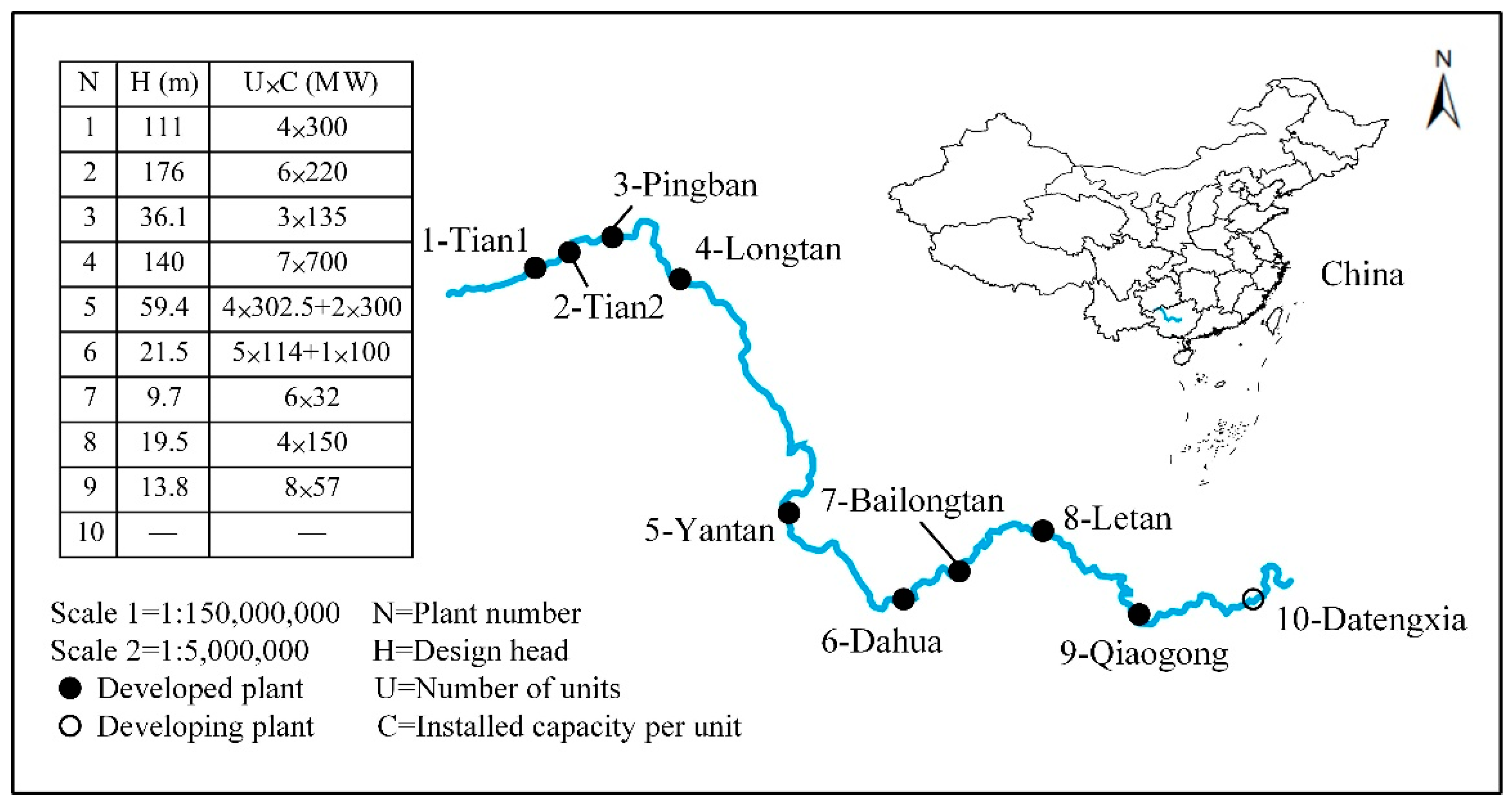
3], especially in Yunnan, Sichuan, and Guangxi provinces. To effectively utilize the water head drop to generate electricity, most of these river basins have adopted cascaded structures, such as the eight-level structure of the middle stream of the Jinsha River and the ten-level structure of the Hongshui River. However, most of the downstream plants in cascaded hydropower systems are often low-head hydropower plants with poor regulation performance (take the Hongshui River cascade structure shown in
Figure 1 as an example, where Pingban, Dahua, Bailongtan, Letan, and Qiaogong are such hydropower plants).
Although the construction of cascaded hydropower plants has greatly improved power generation efficiency, the forebay water level of the downstream plant is greatly affected by the water release of the upstream plant, resulting in large variations in the water head during a single day. Moreover, the power outputs of these plants are very sensitive to water heads [
4]. For head-sensitive cascaded hydropower plants (HSCHPs), inaccurate consideration of water heads will lead to deviations between the planned and actual power outputs, which pose a threat to the safety operation of the power system. In addition, limited by poor regulation performance, water spillage is inevitable when HSCHPs participate in short-term scheduling during the wet season. In 2018, the loss of electric quantity due to water spillage was approximately 69.1 billion kWh [
5], almost one fifth of the total power generation in the UK in 2018 [
6]. Due to the construction of many cascaded hydropower plants with poor regulation performance, China’s Sichuan and Yunnan provinces generate lots of water spillage during the wet season. From 2013 to 2018, the loss of electric quantity due to water spillage in Sichuan increased from 2.6 billion to 12.2 billion kWh, and that in Yunnan increased from 5 billion to 17.5 billion kWh [
7]. In view of the serious electric quantity loss, how to avoid or fully utilize water spillage is one of the hot issues faced by hydropower scheduling in China.
Simultaneously, with the rapid development of the Chinese economy, the peak–valley difference in power loads has increased sharply, leading to increased operational costs and operation risks for power systems [
8]. The large-scale input of fluctuating and intermittent energy sources (such as wind power and solar power), which are not adjustable, further intensifies the peak-shaving pressure [
9,
10]. The maximum peak–valley difference in large and medium-sized cities is approximately 50% of the maximum load. Hydropower, which is characterized by rapid load tracking and flexible regulation, is a high-quality peak-shaving power supply [
11]. Generally, peak shaving is achieved by the hydropower plants with good regulation performance. In fact, for hydropower plants with poor regulation performance, adjusting the water spillage volume at different periods during the wet season can also achieve a better peak-shaving effect. This paper mainly studies the impact of the strategy of adjusting water spillage on peak shaving.
Actually, short-term hydropower system peak-shaving scheduling is a challenging problem due to the complex solution of the objective function and the consideration of the grid, reservoir, and unit constraints. Studies of this problem have received much attention. Simopoulos et al. [
12] proposed an enhanced peak-shaving method to solve the hydro sub-problem, resulting in a modified load curve. Xie et al. [
13] used the peaking demands as constraints to improve the benefit maximization model. Su et al. [
14] formulated a short-term peak-shaving model for cascaded hydropower plants to satisfy the complex demand for the scheduling of grid-connected units. The problems of multiple-grid peak shaving were studied, and several methods were proposed to implement different peak-shaving requirements [
15,
16,
17]. The aforementioned studies can relieve the peak-shaving pressure, but there are still some limitations.
Most studies directly solve the peak-shaving objective function and rarely analyze the peak–valley characteristics of the load curve, sometimes leading to convergence failure. To avoid the above problem, we first accurately divide the peak and valley periods of the load curve before solving the peak-shaving objective function. The division of peak and valley periods based on subjective experience alone is accompanied by human error and, therefore, a more accurate division method is needed. Peak and valley periods have certain aggregation characteristics according to different load values, suitable for division by cluster analysis, which classifies the given data into similar overlapping or non-overlapping groups [
18]. Since the dividing line between peak and valley periods is blurred, it is more suitable to use fuzzy cluster analysis (FCA) for automatic identification, which has been widely applied in the field of meteorology, and computer networks [
19,
20,
21].
Moreover, the existing studies mostly focus on peak shaving during the dry season and wet season without water spillage. In fact, when the incoming water during the wet season is relatively large, for HSCHPs with poor regulation performance, water spillage is unavoidable. HSCHPs usually give priority to economic benefits and mostly aim at increasing power generation during the wet season. Therefore, we consider improving the peak-shaving effect of HSCHPs by adjusting the water spillage volume at each period without significantly affecting the power generation. In this paper, a spillage adjustment strategy called the strategy of releasing water spillage in advance (SRSA) is proposed to increase the power output during peak periods by reducing water spillage.
Mathematically, the short-term scheduling problem of cascaded hydropower plants can be classified as a complex constrained optimization problem with high dimensionality, nonconvexity, nonlinearity, and spatiotemporal coupling [
22,
23]. Moreover, various methods have been developed to solve this type of problem, including dynamic programming and its improved algorithms [
24,
25,
26], and heuristic algorithms [
27,
28,
29,
30]. Dynamic programming suffers from the well-known “curse of dimensionality” as the problem scale expands [
31] and is generally not used to solve peak-shaving models. The improved algorithms rely on their initial solutions [
32]. Heuristic algorithms are easy to converge to a local optimal or even an infeasible solution and extremely rely on the selection of parameters [
33]. In recent years, mixed-integer linear programming (MILP) has gained increasing popularity in the area of hydropower scheduling due to the availability of better performing and more user-friendly commercial software. MILP has powerful functions for processing mathematical models, and binary variables are introduced to linearize complex nonlinear constraints [
34]. Given the sensitive hydraulic connections and complex water spillage constraints in HSCHPs, MILP is selected to solve the short-term peak-shaving scheduling problem.
In the short-term peak-shaving model of HSCHPs, there are some nonlinear constraints which are difficult to solve directly with MILP. Piecewise linearization is commonly used to deal with nonlinear constraints by MILP. Most nonlinear constraints can be linearized directly, and the more difficult one is the hydropower output function, which is a nonconvex two-dimensional function. The piecewise linear approximation of this function is achieved in two ways: using a set of one-dimensional functions for approximation or using meshing and triangulation techniques. Unfortunately, the calculation accuracy of the former is insufficient, and the solution efficiency of the latter is affected because many binary variables are introduced [
4,
35,
36]. Considering the computational accuracy and burden, we follow the basic idea in [
37] and replace constraints with binary variables with a special ordered set of type two (SOS2), i.e., a set of variables of which at most two can be nonzero and these two variables must be adjacent in the order given to the set [
38].
This paper focuses on proposing a novel short-term peak-shaving method considering load characteristics and water spillage for the peak-shaving operation of HSCHPs with water spillage. In brief, the method has three features: (1) FCA is used instead of subjective experience to divide peak and valley periods of the load curve before directly solving the peak-shaving objective function; (2) SRSA is proposed to improve the peak-shaving ability of HSCHPs with water spillage by discarding water during peak periods in advance; and (3) the hydropower output function is approximated by the meshing technique combined with SOS2 to develop a model-based MILP for determining the optimal scheduling program.
3. Methods
3.1. Automatically Dividing Peak and Valley Periods via FCA
Peak and valley membership determines the correlation between the load at a certain period and the peak and valley loads of the day, regardless of the specific load at this period. The day is divided into
T periods and the periods are recorded as
, and the corresponding load values are
. As presented in Equations (22) and (23), the large semitrapezoid membership function determines the membership
of the load during period
t corresponding to the peak load, and the membership
of the load during period
t corresponding to the valley load is determined by the small semitrapezoid membership function [
40].
where
and
are the maximum and minimum loads over all periods, respectively.
FCA is mainly divided into the following steps.
Step 1: Establish and standardize a peak–valley membership matrix.
Use the peak and valley membership of each period
as the statistical index to obtain a peak–valley membership matrix
and standardize
according to Equation (24) to get a standardized peak–valley membership matrix
.
Step 2: Establish a fuzzy similarity matrix.
Determine the similarity
of
and
by Equation (25), and construct a fuzzy similarity matrix
.
where
c is a constraint variable;
; and
.
Step 3: Dynamic clustering based on a fuzzy equivalent matrix.
is squared in turn, i.e.,
. When
appears for the first time,
is the required fuzzy equivalent matrix (transitive closure), which is expressed as
.
where
.
Let
equal any element value in
(from maximum to minimum) to obtain the
truncation matrix
of
.
where
The column vector of corresponds to the element in . When some elements in are of the same type, the corresponding column vector in must be equal. As decreases from maximum to minimum, dynamic clustering is performed.
Step 4: Threshold determination.
Actually, is gradually reduced from 1 for dynamic clustering until the number of clusters is 3, and the automatic division results for the peak, flat, and valley periods are obtained. In practical applications, the peak, flat, and valley periods’ durations should be generally not less than 2 h.
3.2. Strategy of Releasing Water Spillage in Advance(SRSA)
Currently, HSCHPs mainly pursue the power generation benefit and often generate water spillage when the incoming water is particularly large during the wet season due to poor regulation performance. The amount of water spillage can be controlled by the gate. Simultaneously, the short-term scheduling of the power grid is faced with huge peak-shaving pressure because of the shape of the peak–valley difference. It is necessary to reasonably utilize the water spillage of HSCHPs to obtain greater peak-shaving benefits during the wet season. Therefore, SRSA is proposed to increase the power output during peak periods by reducing the water spillage during peak periods.
According to the principle of water balance, when the forebay water levels at the beginning and end of the scheduling period are fixed and the incoming water is determined, the water release during the scheduling period is also fixed. In the actual scheduling (AS) of HSCHPs during the wet season, water at each period is generally released evenly to generate electricity. For HSCHPs, to improve the power generation benefit, whether it is the dry season or wet season, it is necessary to place the operating water level near the highest position because the power generation heads are the largest and the power generation is also the largest under the same incoming water condition. To improve the peak-shaving benefit, the proposed SRSA is to release more water during valley periods, thereby reducing the water release during peak periods. Judging by the relationship between the water release and the tailrace water level, the tailrace water levels are also reduced, resulting in an increase in the power generation heads, thereby increasing the power output during peak periods.
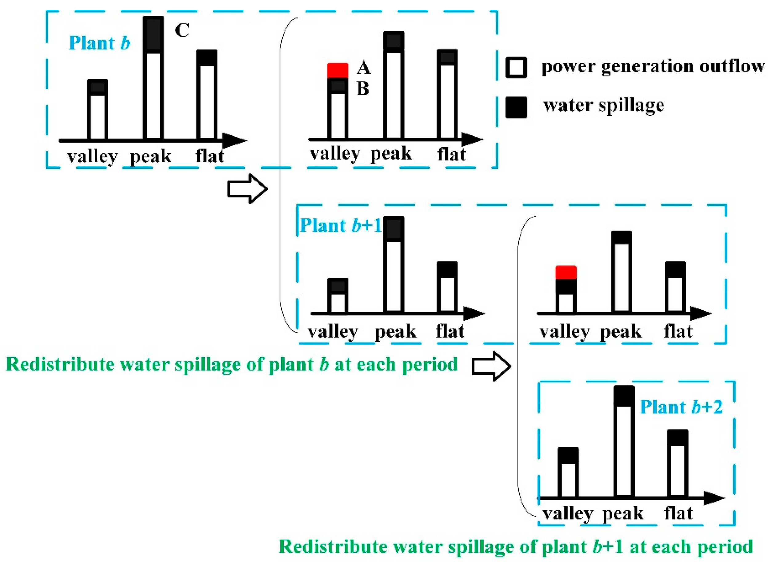
The adjustment process of SRSA is shown in
Figure 2. SRSA is a further adjustment based on the water spillage results of AS. In SRSA, the concept of the water spillage ratio (WSR) is introduced, i.e., the ratio of water spillage that is released in advance to the original total water spillage in a certain period. For plant
b, after redistributing the water spillage, the water spillage during valley periods consists of two parts: the original water spillage (“B”) and the water spillage from the peak periods (“A”); WSR is equal to A/C. Under the condition of constant power generation outflow, during valley periods, the power output of plant
b decreases due to the increased tailrace water levels. In other words, part of the power output of plant
b during valley periods is sacrificed in exchange for the increased power output during peak periods, thereby alleviating the peak period pressure. According to the water release of plant
b after adopting SRSA, the optimal water spillage of plant
b that makes the objective function relatively optimal can be calculated without making changes to other plants. When the water release of plant
b is known (the water spillage and power generation outflow are known), the total inflow of plant
b + 1 is determined and the water release can also be obtained. The same operation is performed on plant
b + 1 to calculate the optimal water spillage of plant
b + 1. After adjusting the water spillage of all plants, the optimal spillage adjustment program is determined so that the power output results of all plants are obtained.
In the proposed strategy, there is no change to the water release during flat periods. The reasons are as follows: first, if more water is released during valley periods, the power output during valley periods will be further reduced, affecting the daily total power generation; and second, limited by the reservoir storage and tailrace water level, the water that can be released during valley periods is certain, meaning that if SRSA is also carried out during flat periods, the water spillage from the peak periods may be reduced.
3.3. Steps for SRSA
The SRSA for HSCHPs should be carried out from the upstream plant to the downstream plant, according to the following process:
- Step 1:
The plant currently being adjusted for water spillage is recorded as b, and the total number of plants with water spillage is recorded as B.
- Step 2:
The most upstream plant b = 1, and its original water spillage is recorded as (obtained from AS).
- Step 3:
For plant b, divide the peak periods’ water spillage equally into the valley periods according to Equation (29) to calculate the adjusted water spillage, , and the original water spillage of plant b + 1, , by the proposed model.
- Step 4:
If , and jump to Step 3, otherwise go to Step 5.
- Step 5:
End the adjustment process.
where
and
are the water spillage of plant
b during period
t before and after adjusting the water spillage, respectively;
,
, and
are the peak, flat, and valley periods, respectively;
is the extra water spillage for each valley period;
is the sum of the number of valley periods; and
is the WSR during period
t,
, i.e., the ratio of water spillage released in advance to the total water spillage during period
t. In principle, the value range of
is
, but in fact, its range depends on the reservoir storage and tailrace water level limits of the plants. The optimal
can be calculated by the optimization model.
3.4. Linearization of Hydropower Output Function Based on SOS2
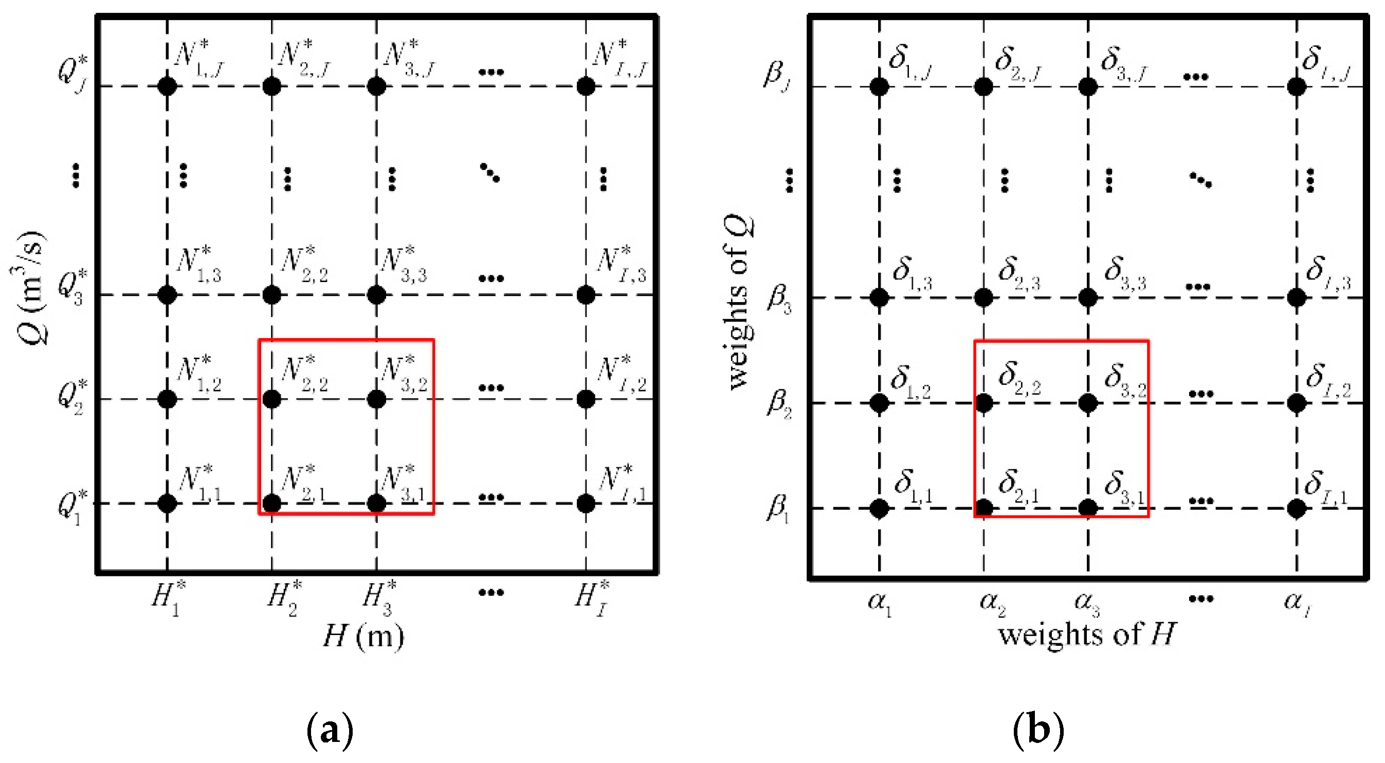
There are some nonlinear constraints, most of which can be achieved by simple linear equations, such as the relationship between the storage and forebay water level, the relationship between the tailrace water level and water release, and the relationship between the head loss and power generation outflow, in the short-term peak-shaving scheduling of HSCHPs with poor regulation performance. In particular, the hydropower output function is a typical nonconvex, nonlinear two-dimensional function, which is troublesome to linearize. In this paper, the meshing technique combined with SOS2 is used to linearize the hydropower output function since special ordered sets are well used in the linearization of the two-dimensional function [
41]. As
Figure 3a shows, the hydropower output function in Equation (18) is represented by grid values by discretizing the water head
H into
I points from the maximum to the minimum
and the power generation outflow
Q into
J points from the maximum to the minimum
. The non-negative auxiliary variable
in
Figure 3b is used as the weight of the power output
in
Figure 3a.
The specific modeling is as follows:
where sets
and
are SOS2 sets, which do not increase the number of variables.
Equations (34)–(36) express the point
as a convex combination of
and
. According to the characteristics of SOS2 (at most, two variables in the set are nonzero and they must be adjacent), only four neighboring grid points can be nonzero and the point
is confined to the interior of these four spatial grids. As shown in
Figure 3b, for instance,
,
,
, and
are nonzero, while all others are zero, meaning that only
,
,
, and
are nonzero in
Figure 3a. When the number of rasterized grid points is sufficient, the point
will infinitely approach the given output function surface.
3.5. Overall Solution Process
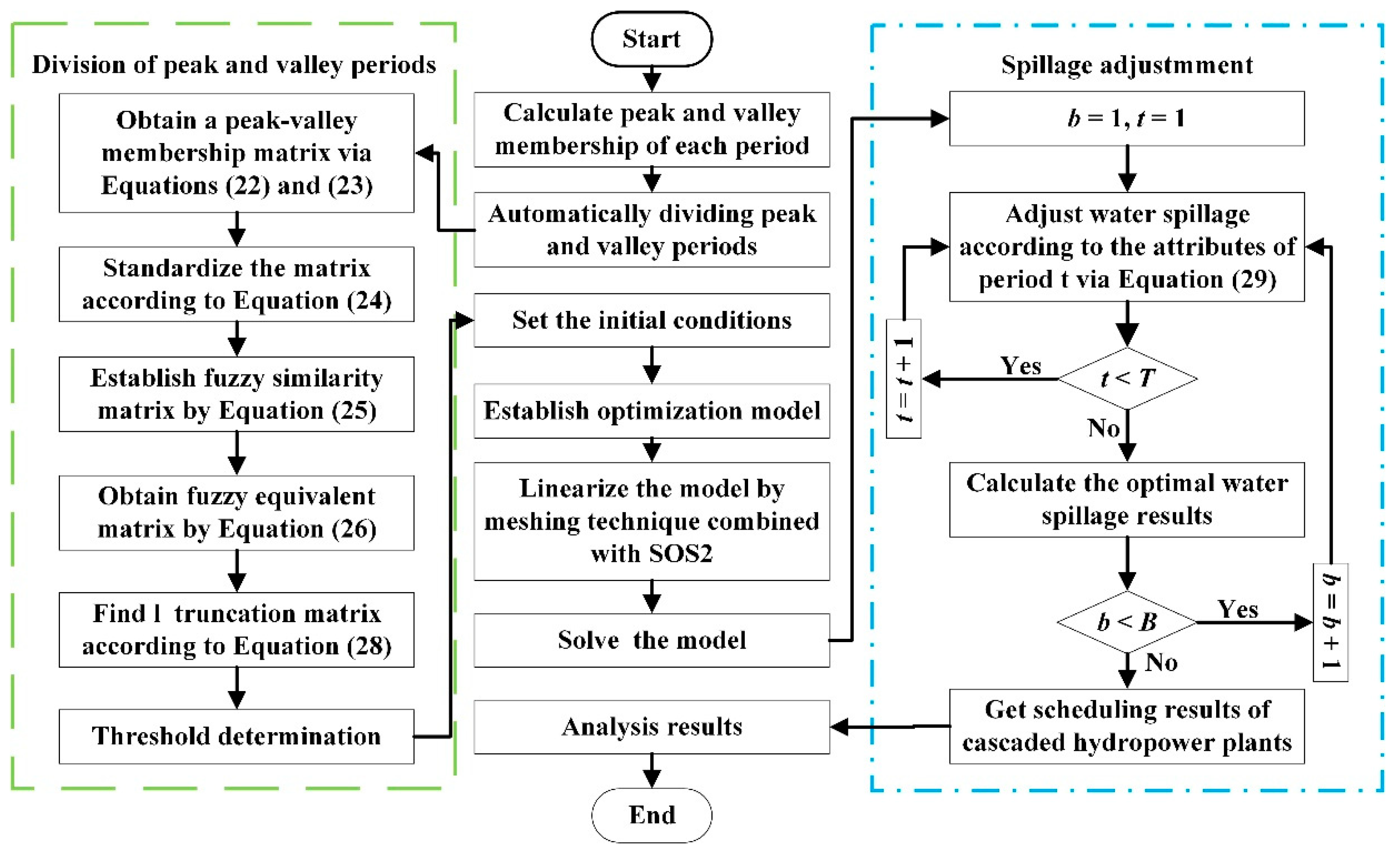
To reduce the peak–valley difference, a novel peak-shaving method considering load characteristics and water spillage for the peak-shaving operation of HSCHPs with water spillage is proposed. The overall solution process of the proposed method is presented in
Figure 4. First, the automatic division of peak and valley periods is carried out by FCA, i.e., the green line in
Figure 4. Then, the linearization of the model is achieved by the meshing technique combined with SOS2. Final, the optimal scheduling results are obtained to achieve an improved peak-shaving effect by SRSA, i.e., the blue line in
Figure 4. The model presented in the previous section is solved with Lingo (17.0
64), a modeling language widely used for optimal scheduling.
4. Application in the Hongshui River Basin
The Hongshui River, one of the first thirteen hydropower bases in China, is located in the upper reaches of the Xijiang River in the Pearl River Basin, with a total length of 1050 km. The total fall and annual average water volume are 760 m and 130 Gm3, respectively, meaning rich hydropower resources. There are 10 hydropower plants that are expected to be built in the Hongshui River, including 1 multiyear regulating hydropower plant, 2 annually regulating hydropower plants, 6 daily regulating hydropower plants, and 1 run-of-river hydropower plant. Currently, all hydropower plants except Datengxia are operational and generating some quantity of water spillage.
Pingban and the cascaded system consisting of Dahua, Bailongtan, Letan, and Qiaogong were selected as study cases to test the feasibility and validity of the proposed method, as shown in
Figure 1.
Table 1 lists the boundary conditions of the selected plants.
In this paper, the initial and terminal forebay water levels of each hydropower plant were set at the maximum to obtain as much power generation benefits as possible in the current scheduling period and the next scheduling period.
When each selected power plant releases water according to its maximum generation flow value, the time required for the reservoir storage from maximum to minimum is listed in
Table 2. The adjustable storage is the difference between the maximum storage and minimum storage. Obviously, when each selected hydropower plant generates electricity at the maximum generation flow without considering the incoming water, the forebay water level falls from the maximum to the minimum within a few hours, demonstrating that the forebay water level is quite sensitive during the scheduling period. In other words, the selected plants are all head-sensitive hydropower plants.
5. Results and Discussion
5.1. Identification of Peak, Flat, and Valley Periods
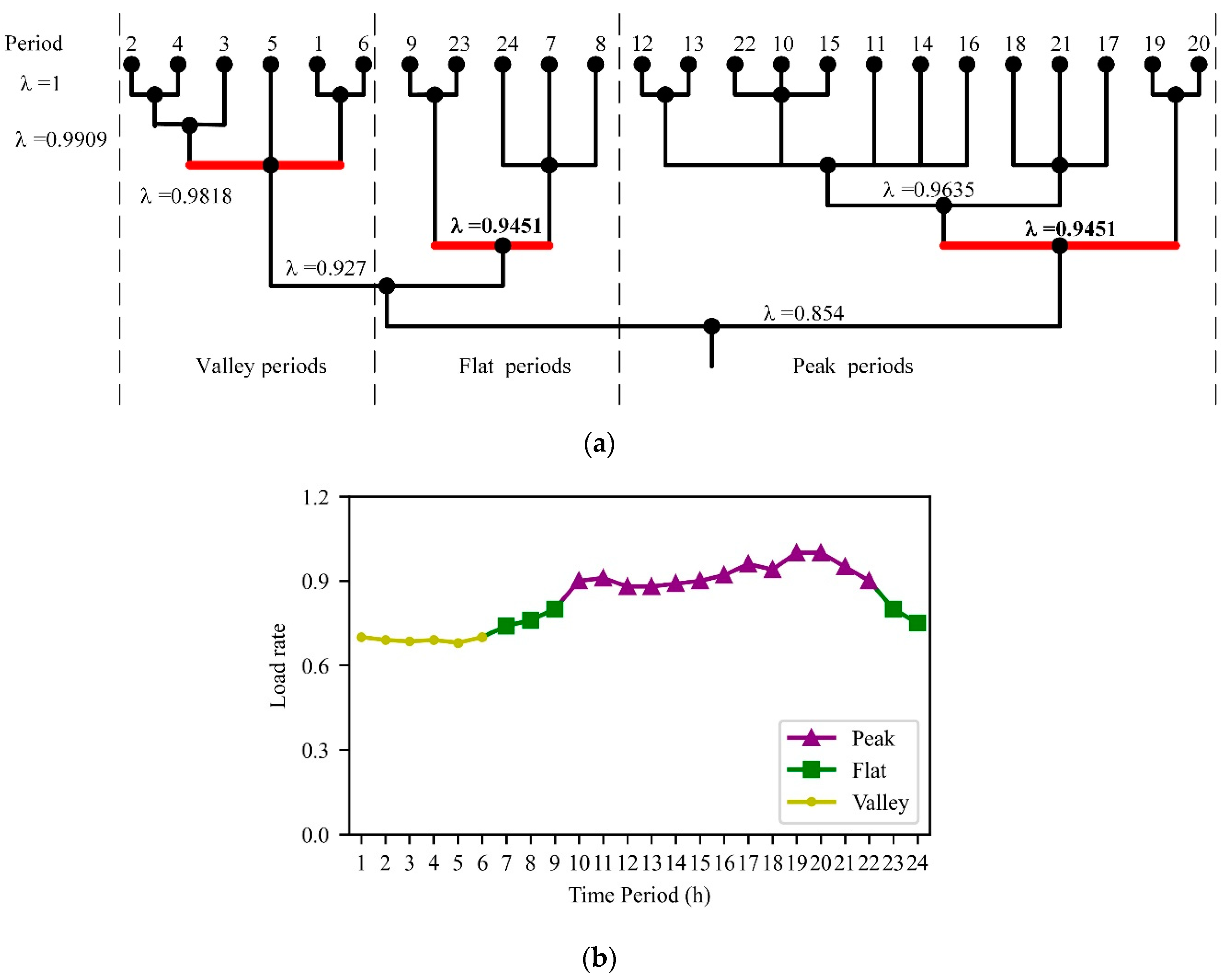
Since Hongshui River enters the wet season in July, HSCHPs’ incoming water is abundant, accompanied by serious water spillage and blocked head problems. Consequently, one day in July with a large amount of steady incoming water (to make the results more intuitive) was selected. The peak–valley difference is 22,966.08 MW, accounting for approximately 32% of the maximum load during the day. The valley periods must be identified before the use of SRSA. FCA, in which
c = 0.1, was chosen to divide the peak, flat, and valley periods. From
Figure 5a, the number of clusters is 3 when
is reduced to 0.9451. Periods 10–22 are peak periods; periods 7–9 and 23–24 are flat periods; and periods 1–6 are valley periods. The classification results satisfy the requirement that the peak, flat, and valley periods are not less than 2 h.
5.2. Case 1—Single Plant
Before verifying whether the short-term peak-shaving method was helpful for cascaded hydropower plants, a single hydropower plant was tested to show how the method works. In order to show the advantages of the proposed method, the scheduling with the proposed method (SPM), AS, and scheduling achieved only by solving the objective function (SAF) were compared. The initial and final forebay water levels and the incoming water are determined, therefore, the water release is certain. Thus, the ratio of water spillage to water release was used to indicate the total water spillage volume of the plant.
Pingban, a typical daily regulating hydropower plant, was selected to prove the effectiveness of SPM.
Table 3 presents the results of the SPM, AS, and SAF of Pingban. As shown in
Table 3, compared to AS, the peak-shaving capacity of SPM increased from 0 to 39.81 MW (9.8% of the installed capacity), and the object value of SPM decreased from 7075.97 to 7064.21 MW. Moreover, the ratio of water spillage to water release of SPM was consistent with that of AS, showing that SPM did not add additional water spillage. Compared to AS, SPM lost part of the daily total power generation, but SAF lost more. Although the peak-shaving capacity of SAF was greater than that of SPM, it sacrificed more daily total power generation and added extra water spillage (27.1%). In comparison, SPM achieved a certain peak-shaving effect while preserving more power generation and did not generate additional water spillage, which was more in line with an economic operation.
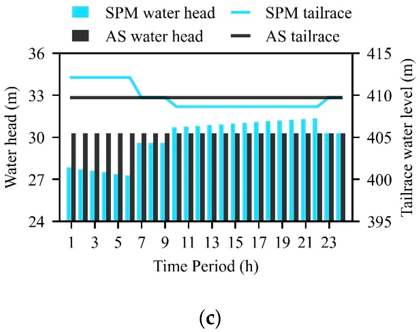
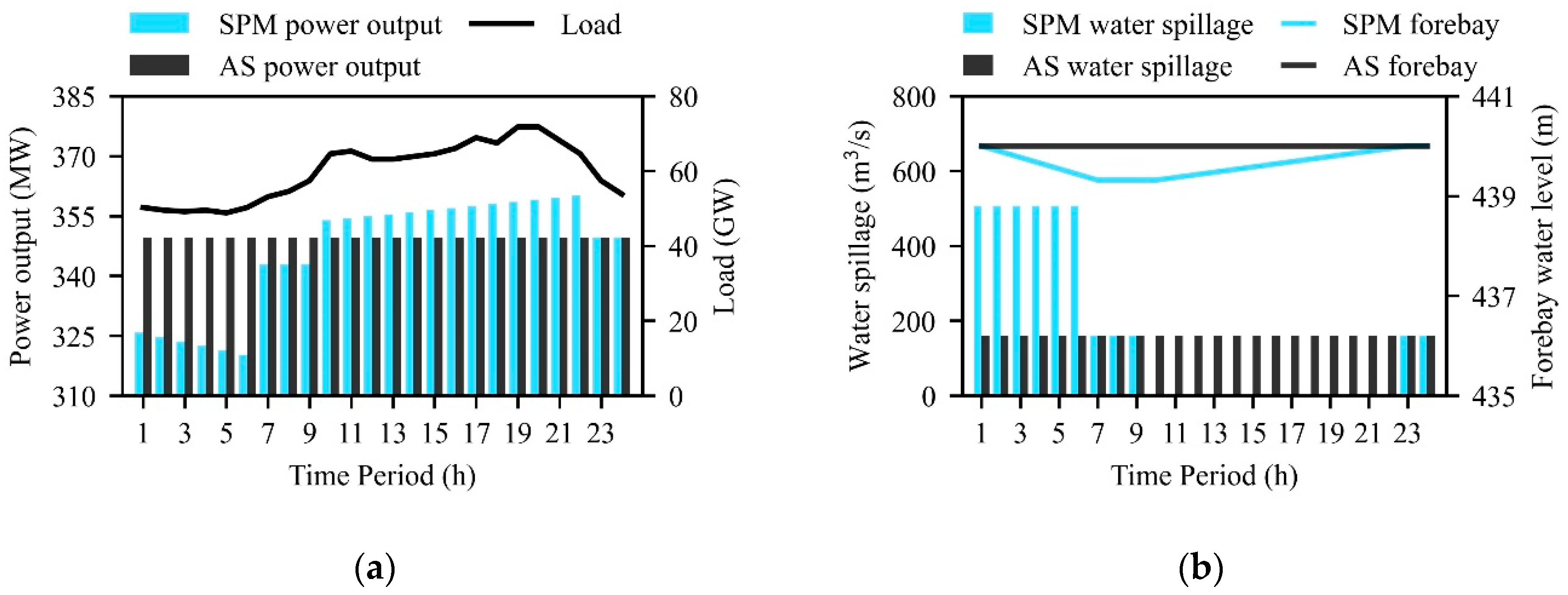
The results of SPM and AS are compared in
Figure 6. By SRSA, the water spillage during peak periods (periods 10–22) was reduced, that of the valley periods (periods 1–6) was increased, and that of the flat periods (periods 7–9 and periods 23–24) was unchanged, reflected in
Figure 6b. Since the power generation outflow was unchanged, the change trend of water release is the same as that of water spillage. The water release during each period met the ecological flow constraint.
For periods 1–6, as more water was released, the tailrace water levels increased and the forebay water levels decreased, leading to decreased water heads; assuming that the power generation outflow was unchanged, the power outputs decreased. Similarly, for periods 11–22, the water release was reduced, thus the tailrace water levels decreased. Although the forebay water levels were not as high as those of AS, the water heads were generally higher, resulting in increased power outputs. As the forebay water level gradually increased, the water head increased, as did the power output. During flat periods 7–9, although the tailrace water levels were unchanged, since the forebay water levels decreased, the water heads also decreased, leading to decreased power outputs. During flat periods 23–24, the water heads were unchanged, thus the power outputs were also unchanged.
In general, compared to the AS’s results, the daily total power generation of SPM decreased, but the peak period power generation increased, and the proportion of the latter in the former increased from 54.2% to 55.9%. For the selected plant, WSR at each peak period was 100%, meaning no water spillage during peak periods.
5.3. Case 2—Cascaded System
A cascaded hydropower system consisting of Dahua, Bailongtan, Letan, and Qiaogong, the HSCHPs in the Hongshui River Basin, was selected to validate the proposed SPM.
Table 4 shows the results of the SPM, AS, and SAF of the cascaded system. From
Table 4, SPM’s peak-shaving capacity of the selected cascade hydropower system was 668.77 MW (36.9% of the total installed capacity), which exceeded AS’s (0 MW). The peak-shaving capacity of each plant of SPM increased by 26.0%, 13.6%, 43.8%, and 56.8% of their installed capacity, respectively. SPM’s object value (6892.28 MW) was better than AS’s (7075.98 MW). The ratio of water spillage to water release of each plant in SPM was the same as that of AS, showing there was not more water spillage in SPM.
Compared with SAF, SPM’s peak-shaving capacity and object value were not particularly advantageous, but SPM sacrificed smaller daily total power generation. The main reason was that Dahua, Bailongtan, Letan, and Qiaogong in SAF all generated more water spillage. Under the condition that their respective total water release was constant, the increase in water spillage led to a decrease in power generation outflow, which affected the power outputs.
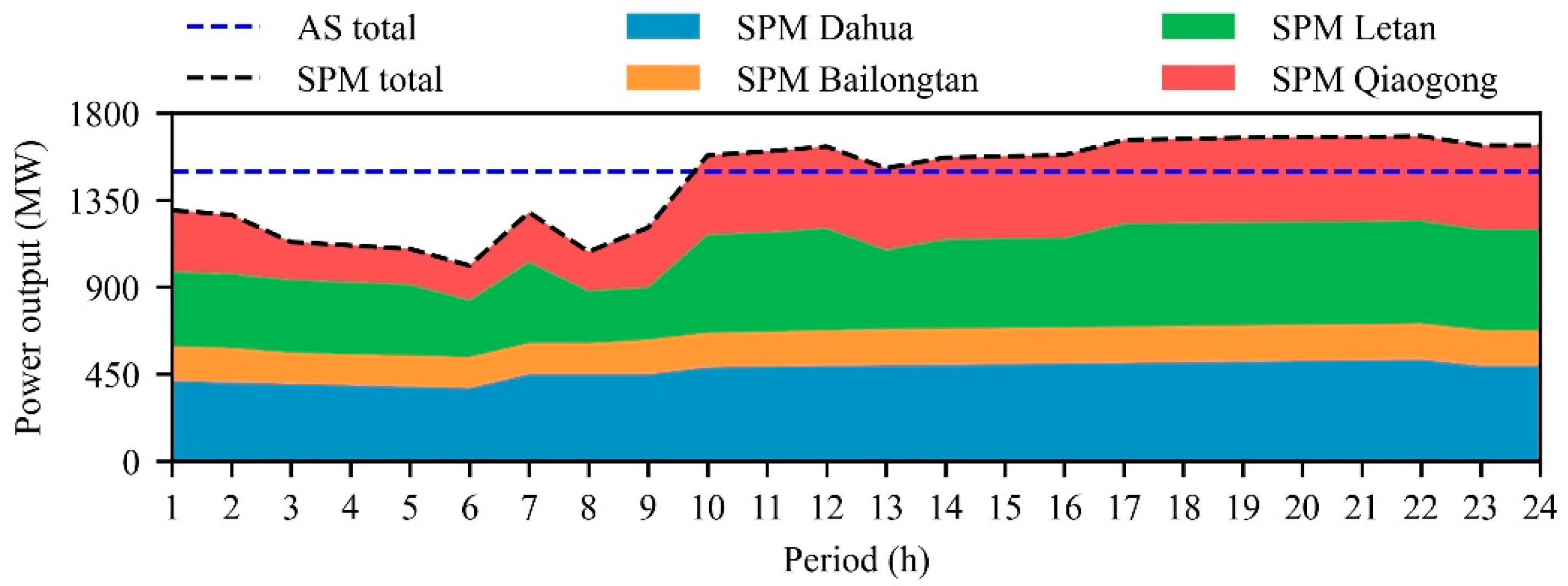
The power output results of SPM and AS for the cascaded hydropower system are illustrated in
Figure 7. The cascaded power outputs during periods 1–10 decreased and those during periods 11–24 increased. On the whole, the peak period power generation increased. In general, from AS to SPM, the daily total power generation decreased by 3.3%, but the peak period power generation increased by 8.3%. The proportion of the latter in the former increased from 54.2% to 60.6%.
In summary, SPM improved the efficiency of peak regulation without significantly affecting the power generation benefits and generating excess water spillage.
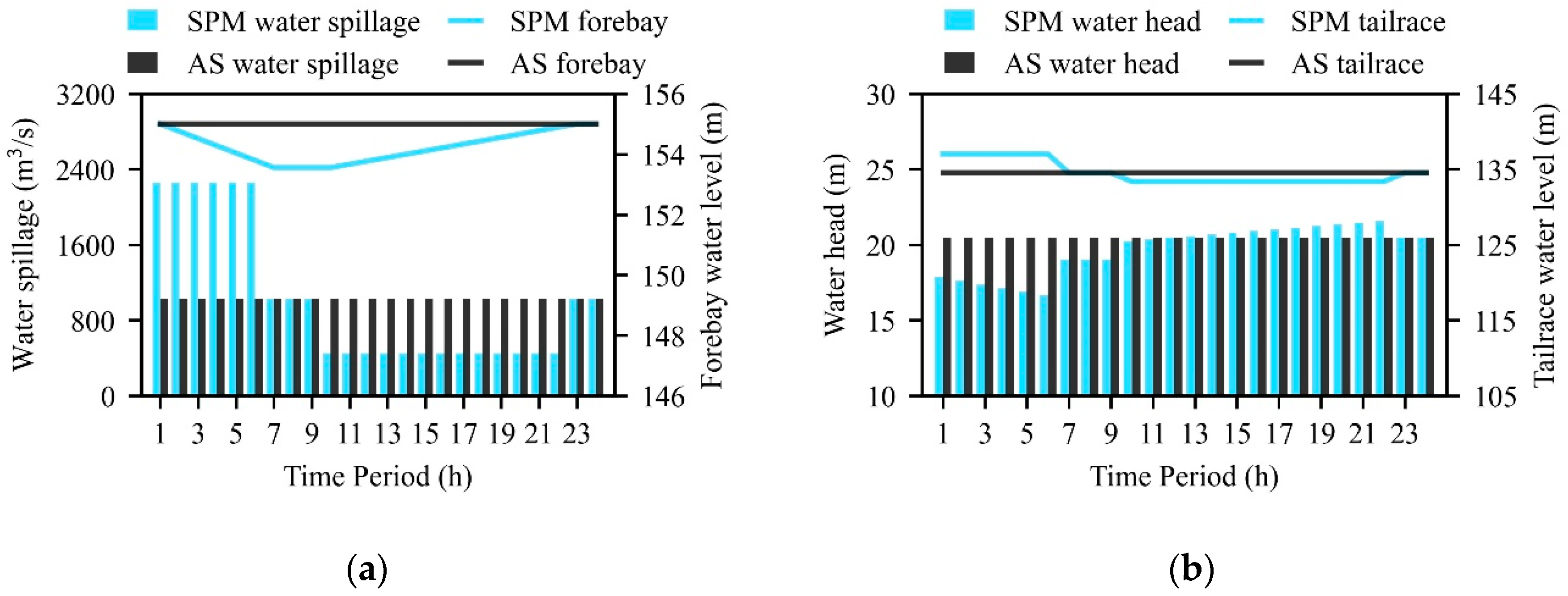
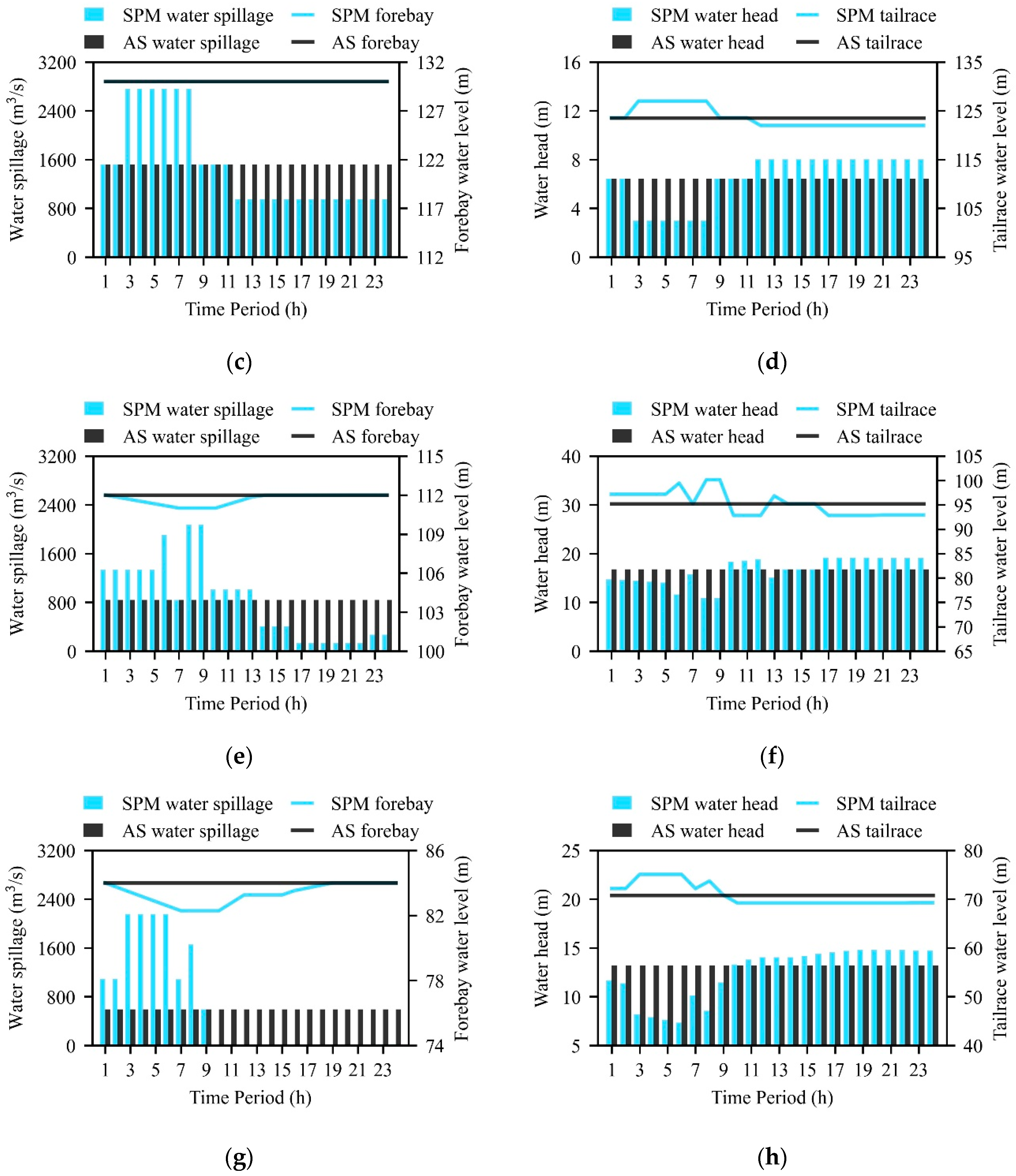
A comparison of water spillage, forebay water levels, water heads, and tailrace water levels between SPM and AS is presented in
Figure 8. Dahua, as the most upstream hydropower plant, was only affected by the adjustment of its own water spillage, thus its optimal operating status was similar to that of Case 1. However, Bailongtan, Letan, and Qiaogong were affected by both the water release of the upstream plant and their own water spillage adjustment. When the water release of the upstream plant changed, the impact on the downstream plant was reflected in a change in the inflow. Affected by the time lag, the optimal water spillage of three downstream plants during certain flat and peak periods after adjusting the water spillage was larger than AS’s. On the whole, the water spillage in most peak periods of each plant was reduced. Adopting SRSA, although the forebay water level and tailrace water level change trends of each plant in the cascaded system were different, their peak period power generation and peak-shaving capacity both increased, as presented in
Table 4. Considering water spillage and power generation outflow, the water discharge during each period of each plant met the ecological flow constraints.
Notably, for Bailongtan, after the water spillage of Dahua was adjusted, the tailrace water levels during peak periods were unsuitable to increase further, limited by the small storage capacity and poor regulation performance. Therefore, the WSRs of Bailongtan during peak periods were 0. Bailongtan was only affected by the water release of the upstream plant.


