1. Introduction
A Water Distribution Network (WDN) is mainly used to distribute water from a reservoir through pipes to fulfil demands of residents. The sum of water demands at these houses determines the amount of water that flows out of the tank. In simple terms, when the amount of water going out of a tank is more than the sum of the demands, then a leak is suspected. The challenge is to locate the leak.
Based on the size, leaks can be categorized into two classes: small leaks and large leaks. Small leaks are defined as leaks with excess flow ≤1 liter per second (lps) [
1], while large leaks are defined as leaks with excess flow >1 lps. Both leaks are detected and localized by utilizing the readings of sensors, for example, pressure and flow sensors. We define the detection and localization of leaks as the
leak quantification. Small leaks are hard to quantify because they do not cause significant changes in flows and pressures in a WDN. Large leaks are easier to quantify, even without the assistance of a sophisticated equipment. This is because large leaks cause significant changes in flows and pressures. Therefore, small leaks tend to persist over a long period that often contribute significantly to the total water losses [
1].
The extra flow going inside pipes caused by a leak must end at the source of the leak seen as the signature of the leak. The signature of leaks at different positions is uniquely indicated by the routes and the magnitude of extra flow on each route. The best way to capture every leak signature at all possible positions in a network is by observing all flows in pipes. This way, we can distinguish the signature of leaks at every location in a network. The drawback of this method is that it requires sensors to be placed on each pipe of the network, which is not feasible due to sensor provision and maintenance costs. A more feasible way to capture leak signatures is by observing flows only at selected pipes. However, this method is quite challenging as small leaks influence only a limited number of flows in pipes. Optimization algorithms are used to find sensor locations that can maximize their functionality.
1.1. Problem Definition
We define the common problems when using sensor readings to quantify leaks as follows:
Given a water distribution network with known demands and a set of k sensors already placed on pipes of the network, what changes in flow would be observed by those sensors for a leak of known size at a known position.
Given a water distribution network and a set of k sensors, how to determine the placement of these k sensors so that leaks can be quantified as accurately as possible. The sensors have not been deployed yet; the solution aims to determine the best possible locations for placing the sensors.
Sensor placement should consider how to accommodate cost-sensitive locations. For example, certain locations with an expensive cost for sensors to monitor than others or locations that are less accessible, should be avoided.
Leaks can occur as single or multiple events. The problem is how do we utilize the k sensors to quantify single and multiple leaks with only limited information about the leaks. To narrow down the scope to conduct maintenance, the uncertainty of the actual leak location must be minimized to the smallest possible area.
How to maintain the performance of leak quantification when data is corrupted due to sensor failures.
1.2. Research Contribution
A set of k sensors detects different flow changes triggered by leaks at different positions. The sensors detect similar flow changes caused by leaks of the same size in a dense area cause, while the sensors detect distinct flow changes caused by leaks of the same size in sparse areas cause (Problem 1). Therefore, the sparser the WDN, the more accurate the leak quantification is. Research focusing on solving Problem 1 exploits existing sensor readings and do not cover the sensor placement problem to maximize the performance of leak quantification.
We focused on solving Problem 2 to 5 when k sensors are not yet placed in a WDN and summarize our contributions as follows:
we develop a novel approach for characterizing small leaks by exploiting flow differences in pipes triggered by such leaks. A directed acyclic graph is used to uniquely describe the signature of a leak, called the lean graph. We maximize the performance of a given number of sensors to quantify small leaks using the lean graphs (Problem 2).
we adjust our approach for managing cost-sensitive locations by re-arranging the locations of sensors while maintaining the performance of leak quantification (Problem 3). The re-arrangement of a sensor is based on the similarities of the lean graphs of the boundary of the cost-sensitive locations.
we utilize the sensors placed by our algorithm to generate dictionaries of leak signatures to quantify single and multiple leaks in small, medium and large water distribution networks (Problem 4).
we enhace our algorithm to tolerate sensor failures and maximize the role of normal sensors by using the subspace voting mechanism (Problem 5).
Our algorithm is developed based on data produced by a simulator (EPANET [
2]) from real water distribution network models. Thus, the limitation of the simulator also applies to the development of our approach. This paper only considers an already-occurred leak. Leak prevention, such as pipe deterioration or blockage detection [
3], is beyond the scope of this paper. The rest of this paper is organized as follows: the review of research related to leak quantification in water distribution networks is presented in
Section 2, the methodology of our research (small leaks simulation and modeling, the sensor placement strategy, single and multiple leaks quantification and fault tolerance) is presented in
Section 3, the experimental results are presented in
Section 4, the discussion is presented in
Section 5 and finally the conclusion is presented in
Section 6.
2. Related Works
Leak quantification techniques have evolved from mathematical modelling to machine learning algorithms. Mathematical modelling simulates the features of the hydraulic system of an operational WDN by using non-linear equations [
4]. Mathematical modelling is more suitable for small-scaled networks due to its nature, which requires large computations. The computational cost can grow significantly when the mathematical modelling is applied to quantifying leaks in large-scale networks. Machine learning algorithms extract an unseen model from a set of data [
5] used to quantify leaks, such as genetic algorithms [
6,
7], support vector machines [
8] and artificial neural networks [
9,
10]. Most of the algorithms require a complete knowledge of network conditions to gain their best performances.
In reality, there is only a limited number of sensors provided. Many techniques have been developed to solve this problem by finding locations to optimally place sensors. Research in Reference [
11] quantifies leaks in a small network using Repeated Incremental Pruning to Produce Error Reduction (RIPPER) algorithm that compares flows detected by the sensors and the rules generated by the algorithm. Other research modelled the sensor placement strategy as the reduction of the Minimum Test Cover which (known as an NP-Hard problem) to the Minimum Set Cover problem as proposed in Reference [
12]. A genetic algorithm was used to find optimum sensor locations by comparing junction pressures of leak-free and leaky conditions [
13]. Observed flows in pipes [
12] and pressure in junctions [
13] with the largest differences are selected as the optimum sensor locations. Junction pressures are also used to explore possible locations to place sensors by finding locations with maximum scores of leak quantification functions by using a Depth-First Branch-and-Bound algorithm [
14].
Elaborating network structures to characterize leak signatures has significantly improved the efficiency of sensor placement strategies. The extra flows detected at the main inlet of a WDN, due to leaks at different positions, are different. The difference is due to the accumulative hydraulic resistances of pipes channelling the extra flows from the main inlet to the leak location. This trend can be noticed clearly in big leaks. The variations of extra flows attracted by leaks at different positions can be used to develop a model that maps leak signatures to their locations [
15]. Leaks are quantified by matching the sensor readings at the main inlet to the model.
The state-of-the-art of research in leak quantification in terms of the most efficient use of sensor is demonstrated in Reference [
15] that uses only one sensor placed at the inlet of a WDN, while research in Reference [
16] demonstrated how to manage the variation on demands that could result in an incorrect model produced by an algorithm used to quantify leaks. The research in Reference [
16] minimized the effect of the variation on demands by modeling the demands based on their geographical locations. The two leak quantification algorithms are based on flow sensing that aim to minimize the use of sensors while maintaining their performances. The leak quantification method in References [
15,
16] are mainly designed to quantify big leaks. The performances of the techniques are significantly affected when they are used to quantify small leaks. In addition, only single leaks can be quantified by the techniques. In real situations, multiple leaks can occur simultaneously at different places.
3. Proposed Method
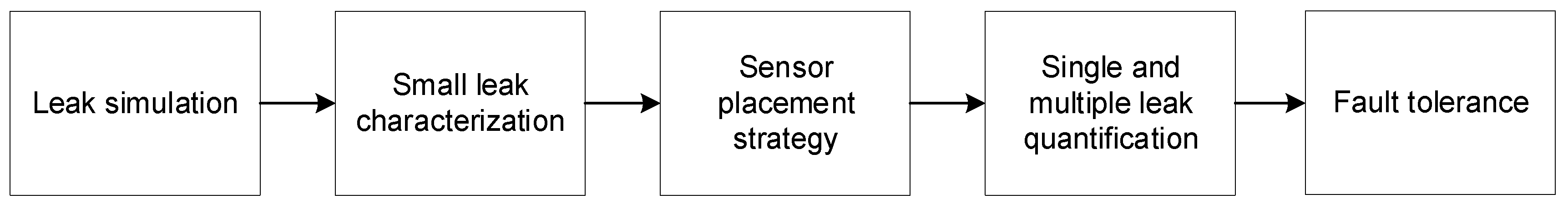
Our methodology consists of the leak simulation, the small leak characterization, the sensor placement strategy, the quantification method for single and multiple leaks and the enhancement of the quantification method to tolerate sensor failures (
Figure 1). We use flow sensors over pressure sensors due to the fact that pressure is more sensitive to measurement inaccuracies than flow [
17,
18].
3.1. Simulating Leaks
Leaks are simulated as an additional demand to the actual demand at a junction. Thus, any junction can be the source of a leak. We use EPANET [
2] to simulate an operational WDN and to generate leak scenarios at different positions. A leak is simulated at a junction by changing the emitter coefficient of the junction to obtain an intended leak size. The emitter coefficient of each junction can be different to simulate the same leak size due to the difference of the physical aspects such as elevation, the distance of the junction to the tank and so forth. Finding a proper emitter coefficient for different leak positions requires a trial-error process. One way to simulate the desired leak size is to use the hill climbing [
19] method. However, this method is inefficient to be implemented for large-sized networks.
To efficiently find the desired leak size, we use the bisection method [
20] to find an initial emitter coefficient for each junction by exploiting the relationship between pressure, emitter coefficient and leak size at the junction. Then, the hill climbing method [
19] is implemented by increasing or decreasing the initial emitter coefficient to simulate a leak at the junction until the desired leak size is met.
3.2. Characterizing Small Leaks
The flow of water in pipes from a tank or reservoir to the furthest downstream junctions forms a non-cyclic system. So, we can model the flows in a water distribution network as a Directed Acyclic Graph (DAG).
Definition 1. Leak-free graph. Let a snapshot of a leak free WDN in a Minimum Night Flow (MNF) be a DAG where V is the vertex set and E is the edge set that represent junctions and pipes respectively. Function maps an edge to flow in a pipe. The direction of the flow is indicated by the direction of the edge e and is the magnitude of the flow in the pipe that functions as the weight of the edge. A model representing flows of the WDN in a leak-free condition is called , where is the set of junctions and is the set of edges. We call this graph as the leak-free graph.
Definition 2. Leak graph. A snapshot of a WDN with a leak at junction x at y lps is modelled as a DAG with the same vertices and edges to (), but the weights and directions of the edges might change. We call this DAG, the leak graph. The direction of the edges in are determined by a function ; a POSITIVE value means the flow direction of edge e in is the same as the corresponding edge in and NEGATIVE means the opposite.
Definition 3. Influence graph. A graph that represents pipes of a WDN influenced by a leak at junction x at leak size y is called the influence graph () whose vertices and edge directions are the same to but the edge weights are different. The edge weights are produced by a function that produces edge weights. POSITIVE value indicates increased flow in pipe i and the flow directions at and are the same. NEGATIVE means the direction of flows in pipe i has flipped or the flow direction in the pipe has not changed but the flow decreased. Zero means a pipe is not influenced by the leak. Note that the NEGATIVE value can be perceived as the directions of an edge has changed at from the corresponding edge at . Therefore, to maintain the actual direction of edges at , we use another function that will give POSITIVE value only if the actual flow direction of pipe i has changed, and NEGATIVE for other conditions. Hence, the weight and direction of the edges at is the result of . By using this approach, the directions of edges at and are consistent. A matrix represents leak sources in rows and influenced pipes in columns, termed as the influence matrix ().
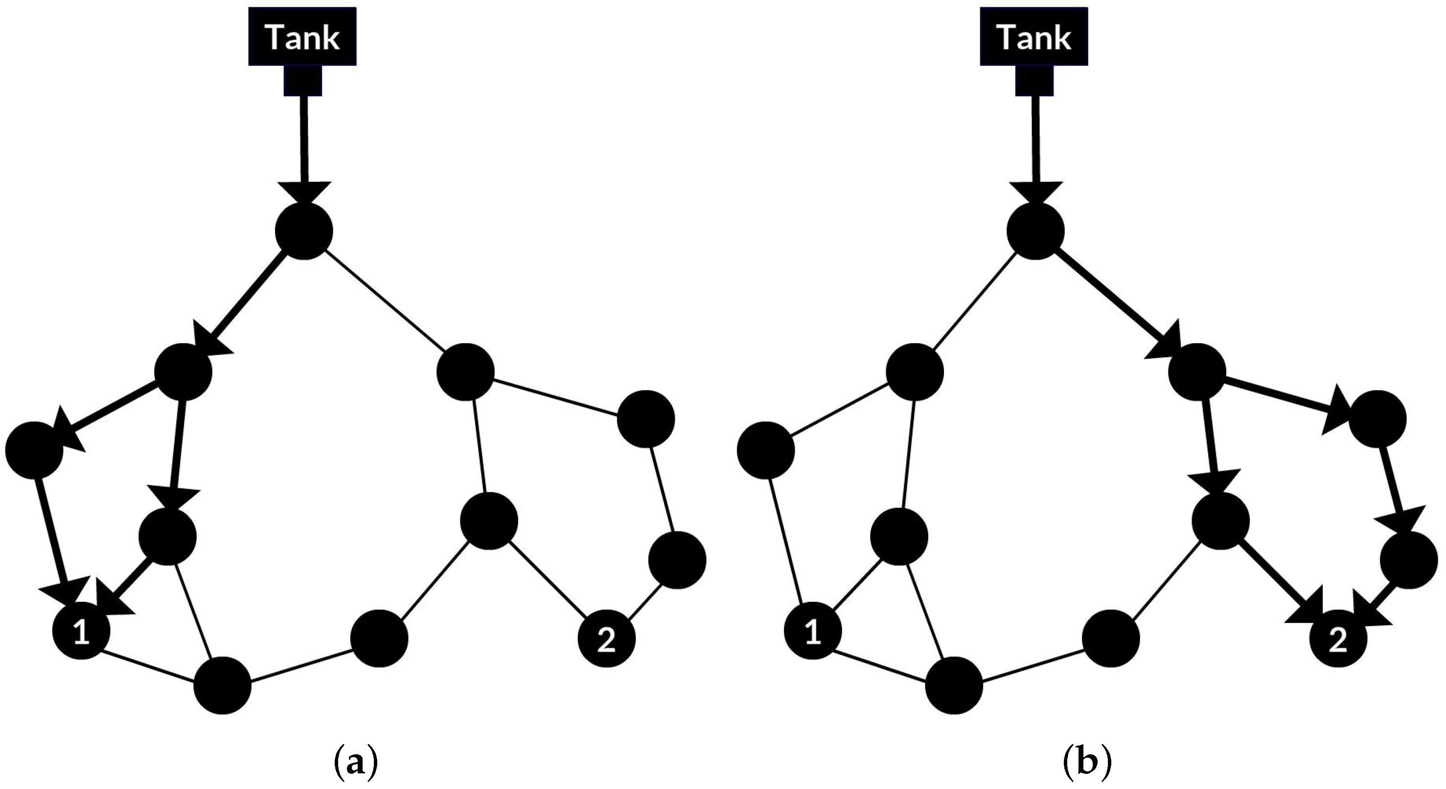
Definition 4. Lean graph. Let be a leak case from . We construct a DAG from each and collect all edges with directing to a leak source at junction x. Thus, creating a path from a tank/reservoir through edges representing pipes with increased or flipped direction flows to the leak location [21]. We call this DAG the Lean Graph () as indicated by the bold edges in Figure 2a,b. Therefore, while the direction and the weight of each edge in is the same as the corresponding edge in . Each lean graph is unique and used to characterize the signature of a leak at a particular position. The size of a leak determines the spread of influenced pipes. The bigger the size, the wider the spread, hence, bigger lean graphs. Bigger lean graphs result in overlapping leak signatures that cause the lean graphs fail to characterize leaks. The thinnest construction for all lean graphs is obtained with the smallest leak that can be simulated in a WDN, called the minimum common leak (MCL) size.
3.3. Sensor Placement Strategy
One way to quantify leaks is by partitioning a WDN into clusters and localizing a leak in a cluster based on certain criteria [
22,
23]. We partition a WDN based on lean graph similarities measured by using the
Jaccard Index (JI) [
24] which divides the intersection of each pair of lean graphs by their union. A
JI table stores the
JI of all lean graph pairs.
3.3.1. Clustering a WDN to Place Sensors
The clustering process starts by finding a centroid () of a cluster selected from a pair of junctions with the highest value in a JI table. Then, a threshold () is set to determine the boundary of the cluster. Connected junctions within the range of from are added into the cluster. Junctions that have been recruited in the cluster are removed from the next cluster formation process to avoid double selection. This procedure is performed for the remaining junctions until all junctions are included in a cluster. Next, an inlet for each cluster is selected from edges at the boundary of a cluster that connects the cluster to its neighbour. An inlet of a cluster is selected from edges at the boundary of a cluster with the highest JI score. The intuition of the criterion is that an edge with a high JI value indicates more intersection of leak signatures. The cluster inlet is used to distinguish the signatures of leaks in the cluster from the signatures of leaks of the other clusters. We evaluate the inlet selection using two measurements:
The best cluster set is the one with the lowest CS and the highest PB. One way to find the optimum cluster set is by using a parameter sweeping technique, that is, by gradually increasing threshold within a given range and step. However, optimizing sensor configurations using parameter sweeping often requires significant computational costs.
To manage this problem, we compare the parameter sweeping method with a randomized selection. The key for finding the optimal clusters is setting the proper . First, the randomized selection algorithm generates an initial to partition a WDN. This is set as the best . An inlet is selected for each cluster, then CS and PB scores are calculated. The CS calculation is performed in pairs. The dot product of each pair of sensor readings is calculated. This procedure is performed until the CS of all possible pair of sensor readings are calculated. Finally, the calculation results are summed to obtain a final CS score. The PB is calculated by summing the entropy of each cluster. These CS and PB are set as the best CS and PB.
In the next iteration, the randomized selection algorithm generates another to find new clusters and their inlets. Then, new CS and PB scores are calculated. If the new CS and PB are better than the previous scores, the new is set as the best , the best CS and PB are updated with the current scores. Otherwise, the previous best , CS and PB are maintained. This process is performed until the iteration limit is reached. Upon reaching the limit, the cluster inlets from the best , CS and PB are used.
3.3.2. Adjusting Clustering Results
The number of inlets to place sensors might not equal the number of sensors provided (k); adjustment steps are performed by partitioning or merging clusters to equalize to k. Partitioning is performed when the number of clusters is fewer than the number of sensors, while merging is performed if the opposite is true. We select the biggest cluster to be partitioned while we merge the smallest cluster to its neighbor with the highest JI score. Partitioning a cluster is performed using the same clustering procedure, but with higher . This procedure results in smaller clusters with higher connectivity which contributes to the higher PB score. Merging a cluster is performed by adding each junction of the smallest cluster to an adjacent cluster with the highest JI score.
3.3.3. Cost-Aware Clustering
Junctions can be in a sensitive area where placing a sensor is not feasible, such as highly secured buildings, expensive or inaccessible locations to deploy sensors. A possible way to accommodate this situation is to find places nearest to the sensitive area to place a sensor. This can be performed in a post clustering phase by grouping junctions in the cost-sensitive area into a cluster and then selecting an inlet for the cluster. A sensor for the inlet of the newly formed cluster is required. The sensor can be obtained by adding a new sensor or relocating a sensor from another cluster with a lower priority. Adding a new sensor increases the precision of leak quantification as it reduces cluster sizes. However, it requires more funding. Relocating a sensor causes the cluster from which the sensor is taken to be dismissed, and the junctions of the cluster are merged to adjacent cluster(s) with the highest JI score.
3.4. Localizing Single and Multiple Leaks
We develop a framework to locate leaks based on matching out-of-normal flows to the records of a leak signature database. When a leak occurs, we can easily find the location of the leak by comparing the current flow changes to the records in a database. One record in the database with the closest match is selected, and the label of the record indicates the location of the leak. The key to our leak quantification framework is to generate sufficient leak signatures in a database.
3.4.1. The Dictionary of Leak Signatures
Leaks affect flow changes in pipes differently depending on the location and size of the leak. The magnitude of flow changes in pipes triggered by a leak creates a unique vector of numbers that distinguishes from the others. Therefore, the unique vector can be regarded as the signature of the leak.
Definition 5. The dictionary of leak signature. Function indicates the influences of a leak at in the selected columns ; with . is the set of inlets and is the set of all pipes in a network. is a matrix that contains the vector of sensor readings where the rows of are the locations of leaks and the columns of are the cluster inlets . In other words, where all rows in are taken from and only columns of that match to are taken. We call the dictionary of leak signatures.
The columns of each row in a dictionary are used to represent the signature of a leak at junction
at
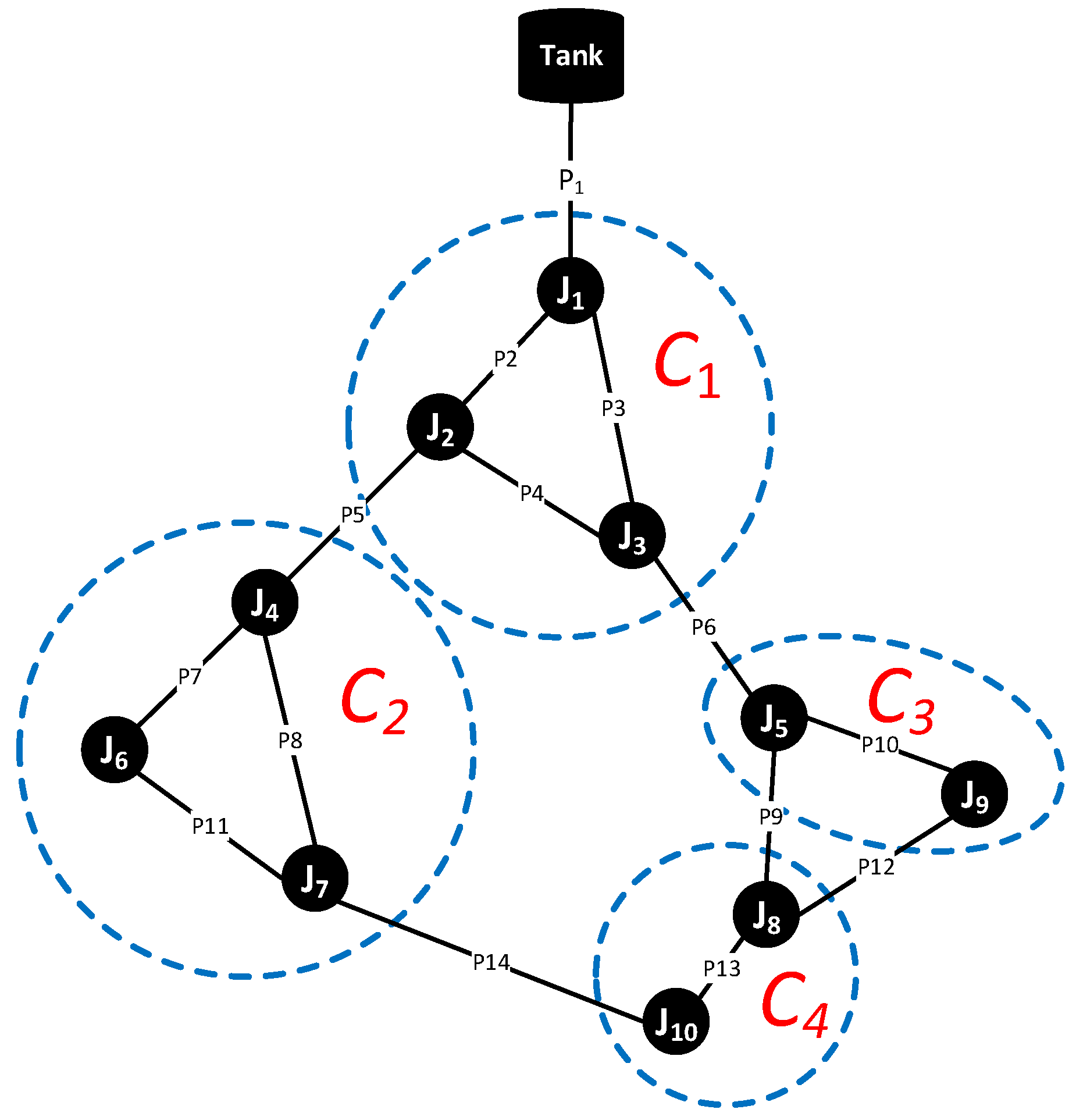
y lps. Consider a simple network with 10 junctions, 13 pipes and one tank (
Figure 3). Suppose there are our sensors to be deployed in the network. We partition the network using our partitioning algorithm (resulting in four clusters) and select the cluster inlets. One sensor is placed at every cluster inlet, namely at
.
acts as the main inlet which detects anomalous extra flows, suspected as the effect of leaks, into a network.
Leaks are simulated at every position in the network at the intended leak size (e.g., 0.2 lps). Flow changes in pipes are stored in an influence matrix. To create a dictionary of leaks at 0.2 lps, we take the columns of the influence matrix which correlate to the cluster inlets (
Table 1). Here, identical vectors are examined, and only one of the identical vectors
in the same cluster is selected to be kept in the dictionary, while the others are dismissed.
3.4.2. Reducing Leak Quantification Uncertainty
A record of a dictionary (
Table 1) quantifies a leak in one cluster. Suppose a single leak is quantified in a cluster consisting of three junctions. Then, a manual method, such as the use of acoustic detector, is then performed to the suspected junctions to find the actual leak location. Some clusters in dense areas could have many junctions that cause high uncertainty for maintenance.
Reducing the uncertainty can be performed by utilizing the distinctiveness of dictionary vectors. The key to accurately quantify leaks is how significant the variations of vectors are in representing the locations of leaks. The more variations, the less quantification uncertainty. We modify our sensor placement strategy by including flow variations detected by sensors () as another criterion in addition to JI to select a cluster inlet. All pipes with are included in the inlet candidate set, while the others are omitted.
Let be a set of cluster inlets selected by considering JI and . A dictionary is constructed by subsetting an influence matrix based on . Pipes in can be the same or different from . Next, any identical vectors in the dictionary are identified regardless of which cluster they belong. One of the identical vectors is to be kept in the dictionary, while the others are omitted. Thus, each vector in the dictionary is unique that refers to one junction or a group of junctions.
Continuing with our example, suppose the set of inlets in
are the same as in
, that is, (
). We notice that the vectors representing leaks at
and
are identical (
Table 1). One vector is selected to represent the leak signature for the two junctions. This procedure reduces the number of vectors in the dictionary by 1 row. The number of distinct vectors in a dictionary grows linearly with the leak size. The higher the leak size, the lower is the quantification uncertainty.
3.4.3. Multiple Leaks Dictionary
We change emitter coefficients at junctions to simulate identical leak sizes at every possible combination of locations. Considering the maximum size of small leaks must not exceed 1.0 lps, the possible range of double leaks is [
] lps constructed from
lps to
lps. The same method applies for triple leaks or any number of multiple leaks. For a network with
n junctions, the number of combinations of possible leak locations is calculated using Equation (
1) where
r is the number of multiple leaks.
We generate influence matrices by recording flow changes from leaks simulated at the combinations of locations at different sizes. Then, we subset the influence matrices at columns corresponding to the sensor locations to generate leak signature dictionaries.
3.4.4. Localizing Leaks
The extra flow detected at the main inlet can be the signature of single or multiple leaks. Since the number of leaks is unknown, every dictionary (single or multiple) that matches the extra flow detected at the main inlet is used to quantify leaks. For example, suppose an extra flow caused by a single leak is detected at lps. Although the extra flow is caused by a single leak, it is unknown to us. Hence, all dictionaries that match to 0.4 lps are selected, that is, single leak dictionary and double leak dictionary , to quantify the leak. The lowest Euclidean distance is calculated between the vector of the single leak against all vectors in the dictionaries. Vectors in each dictionary whose distances are equal to the lowest Euclidean distance are recorded, and the location of the leak is indicated by the labels of the vectors. The hydraulic system causes flow in pipes triggered by single and multiple leaks to differ. Thus, the vectors of should produce lower Euclidean distances than . In only a few cases the distances of the vectors are as low as the vectors of . This quantification method also applies to multiple leaks.
3.4.5. Evaluating the Performance of Quantification
Evaluating the accuracy of the leak quantification is performed by comparing the quantification label against the actual location of a leak. We consider three scorings to measure the performance of quantification:
Score 1 for a correct quantification. A leak at quantified at gives the score of 1. Also, a double leak at and quantified in a group of junctions [] or [] gives a score of 1.
Score for partially correct quantification, where n is the number of correctly quantified leaks and m is the number of leaks. A double leak at and quantified in a group of junctions [] or [] gives the score of .
A score of 0 is given for completely wrong quantification. For example, a double leak at and quantified in a group of junctions [].
3.5. Fault Tolerance
In reality, flow data can be corrupted and can affect the performance of leak quantification. The corrupted data can be caused by sensor failures. The failures can be a sensor that does not give flow detection (termed as the NA sensor), a sensor that consistently gives incorrect flow detection (termed as the biased sensor) and a sensor that gives inconsistent flow detection (termed as the noisy sensor).
Let us refer to the sensor locations in the simple network (
Figure 3). A
NA sensor on
will cause the signature of leaks at
and
to become indistinguishable (
Table 1). A biased sensor produces consistent data, but the value is incorrect. For example, an actual flow at 3.0 lps is consistently detected as 3.05 lps. A noisy sensor generates inconsistent data within a certain range of the actual flow, for example, ±3% [
25]. For example, a 3.0 lps flow is detected within the range of [2.91, 3.09] lps. Biased and noisy sensors do not affect leak signatures as dramatically as a
NA sensor. However, they degrade the quantification performance as they change leak signatures.
NA sensors can be noticed when there is no flow detection, while noisy sensors can be noticed when there are inconsistent flow detections. The problem with NA sensors can be solved by replacing the sensors, while the problem with noisy sensors can be solved by averaging flow detections. Sensor manufacturers have implemented the averaging flow method in their products.
3.5.1. Unnoticeable Sensor Failure
Biased sensors are hard to notice because they always give consistent values of flow detection. They cause shifted leak signatures even when there is no leak in a network. Even though leak signatures are shifted, the composition of the junction(s) owning a vector of leak signature does not change. Only the value(s) of the vector changes. The wider the bias the further the vector is shifted from the correct one.
Bias failure can occur to any of the sensors in a network. A biased sensor at the main inlet does not significantly influence quantification performance. This is because the sensor at the main inlet only detects a constant change of flow indicating the size of a leak or the accumulative size of multiple leaks. The performance of quantification will be more driven by the non-main-inlet sensors. However, a significant bias detection at the main inlet can lead to an incorrect selection of dictionary which eventually affects the quantification performance. For example, a biased sensor at the main inlet with +0.1 lps bias would cause an extra flow of 0.2 lps detected as 0.3 lps. This event will lead to an incorrect dictionary selection and eventually degrade the quantification performance.
3.5.2. Subspace Voting Quantification
The location of a biased sensor is unknown. Therefore, localizing leaks must be performed by using the given data from existing sensors. We created a method to minimize the effect of the biased data called the
subspace voting quantification. A subspace of a vector of leak signature consists of one or some components of the vector. For example, there are 15 subspaces of a vector generated from four sensors placed on pipes
(see
Figure 3), that is,
. In general, there are
subspaces of a vector of length
n. Suppose the sensor on
is biased. Every subspace containing
is not an accurate leak signature while every other subspace without
is.
To quantify a biased leak vector
, the Euclidean distances of every subspace of the biased vector
to the corresponding subspace of all records of a selected dictionary
are calculated. The vote of each subspace of a record of the dictionary with the lowest distance is marked with 1, otherwise 0. Then, the voting scheme takes place by sumarizing the votes of each dictionary record obtained from all subspace marks. All dictionary records with the highest vote are selected and used to quantify the biased vector
. The majority of the vote is expected to result in the correct quantification. However, the effect of the biased data might cause this not to happen. To evaluate the performance of the subspace voting quantification, we aggregate the quantification results of every possible leak vector based on the scoring scheme in
Section 3.3.
The voting method maximizes the role of the accurate subspaces against the inaccurate subspaces. Thus, the method can tolerate corrupted data. However, the method only works if and only if the number of inaccurate subspaces is fewer than the accurate subspaces.
4. Experimental Results
All experiments were purely conducted based on simulations using EPANET [
2]. We conducted our experiments sequentially by performing our sensor placement strategy, localizing single and multiple leaks and applying the subspace voting quantification method to deal with biased sensors.
4.1. Sensor Placement Strategy
We use seven WDNs (
Table 2) in our experiments with typical real-world elements: tanks, pipes, and junctions. Each WDN represents different characteristics that are significant to our sensor placement strategy: the complexity of network structure, demands, connection degree and the number of tanks. The structure of a network and its demands are the basic components to form a lean graph. The connection degree of a network determines how extra flow splits. The higher the degree, the more paths the extra flow can split. Finally, the extra flow can come from one or more of the tanks in the network.
The quality of a cluster set is measured based on two aspects—Cosine Similarity and Partition Balance. We used the parameter sweeping and randomized selection methods to partition a WDN. We compare the performance of both methods based on the CS and PB scores. Parameter sweeping method is an algorithm while randomized selection method is an algorithm on average. Both algorithms will have to perform the graph partitioning and to measure the CS and PB score each time a is generated. The efficiency of the randomized selection method is measured by recording the number of iterations performed compared to parameter sweeping. In parameter sweeping method, we used = [0.01, 1] with a step size of 0.01 that equals 100 iterations. While the randomized selection method, we set the iteration to a maximum of 50.
The computational cost of partitioning process increases along with the increase of network sizes. This trend is noticeable in larger networks as the size of each cluster in this category is commonly larger than that of the smaller category networks. Consequently, more lean graphs are to be processed to find an inlet for a cluster. Here, the role of randomized
selection is significant in reducing the computations. We record the time required to find the optimal
between parameter sweeping and randomized
selection methods and calculate the difference of time required by each method. We regard the time difference as the measurement of the efficiency [
29]. Significant improvements in efficiency are indicated when the randomized
selection method is used (
Table 3).
4.2. Complex Networks
We expand our experiments to find optimal sensor placement by using a more complex network with 388 junctions, 432 pipes, 11 pumps, four valves, seven tanks and one reservoir (the complete C-Town network [
26]). The network is divided into five smaller areas called District Metered Areas (DMA). Each DMA is a
semi-independent network which enables a DMA manager to control incoming and outgoing water to a DMA [
30]. Also, in some range, a DMA can fulfil its demands should the DMA is disconnected from the big network. This characteristic enables leaks to be quantified in a DMA to perform further maintenance procedures while maintaining the fulfilment of its demands [
31].
The inlet of a standalone DMA is the pipe closest to a tank or a reservoir of the DMA. But when all DMAs are connected, we need to identify a pipe that detects the most leak signatures for each DMA which might not be the pipe closest to a tank or a reservoir. One DMA’s Minimum Night Flow (MNF) at a point of time does not always match with the MNF of the other DMAs. Therefore, we find a period of common MNF where the collective demands in all DMAs are minimum. Then, we take the snapshot of the network at the common MNF and use it to construct the leak-free graph (). Then, we introduce leaks one at a time at junctions and construct the leak graphs (), the influence graphs () and finally the lean graphs (). We generate a JI matrix from the lean graphs and use it to select the main inlet for each DMA. Pipes at the boundary of a DMA are listed as the inlet candidates and sorted in descending order based on their JI scores. One pipe with the highest score is selected as the main inlet for the DMA.
4.3. Cost-Aware Clustering
We modify the cluster by grouping junctions in a cost-sensitive area into one cluster, and distribute other junctions which are not in the cost-sensitive area to the nearby clusters. To maintain the least deterioration in sensor placement quality, we accommodate the cost-sensitive areas in the post-clustering process. Some cluster inlets might change after the modification. We compare the quality of the initial and post-modification cluster sets by measuring the CS and PB scores.
Our approach can maintain the quality of the sensor placement indicated by insignificant changes in
CS and
PB, that is, less than 0.1 for both scores (
Table 4). The least changes of
CS and
PB scores is at the multi-tank network (Pescara). The use of sensors at the pipes connected to the tanks preserves the distinctiveness of sensor readings and the balance clusters. This way, the addition of a sensor for a cost-sensitive area has a very small effect on the scores. The results show that not only our approach can find optimal places for sensors, but also it is flexible to accommodate real issues in the implementation.
4.4. Localizing Leaks Using Dictionaries
We simulate single, double and triple leaks to examine our approach. Double and triple leaks are simulated at the same size for each combination of junctions. When a leak occurs, the only information that relates to a dictionary is the change of flow detected by the main inlet, while the type of the leak (single, double, or triple) and the locations are unknown. We use a scheme to select which dictionary to use to quantify leaks (
Table 5). Based on the scheme, all dictionaries that match to an extra flow detected at the main inlet is selected. Suppose a leak is detected at
lps at the main inlet, then dictionaries that can be used to quantify the leak are: single leak dictionary
, double leak dictionary
and triple leak dictionary
. Some dictionaries are not suitable to quantify certain sizes, such as a double leak dictionary to detect leaks at 0.2 lps and 0.3 lps or a triple leak dictionary to detect leaks at
lps,
lps and
lps.
As the baseline, we place five sensors for each network used for experiments. The dictionaries for each network are constructed from the five sensors. For testing purpose, we randomly generated 20 cases of every possible size of single, double and triple leaks. We measured the Euclidean distances of leak vectors to the vectors of the selected single, double and triple dictionaries. We use Beckenham network to describe the general experimental results as this network has the most balanced complexity among the other networks (see
Table 2).
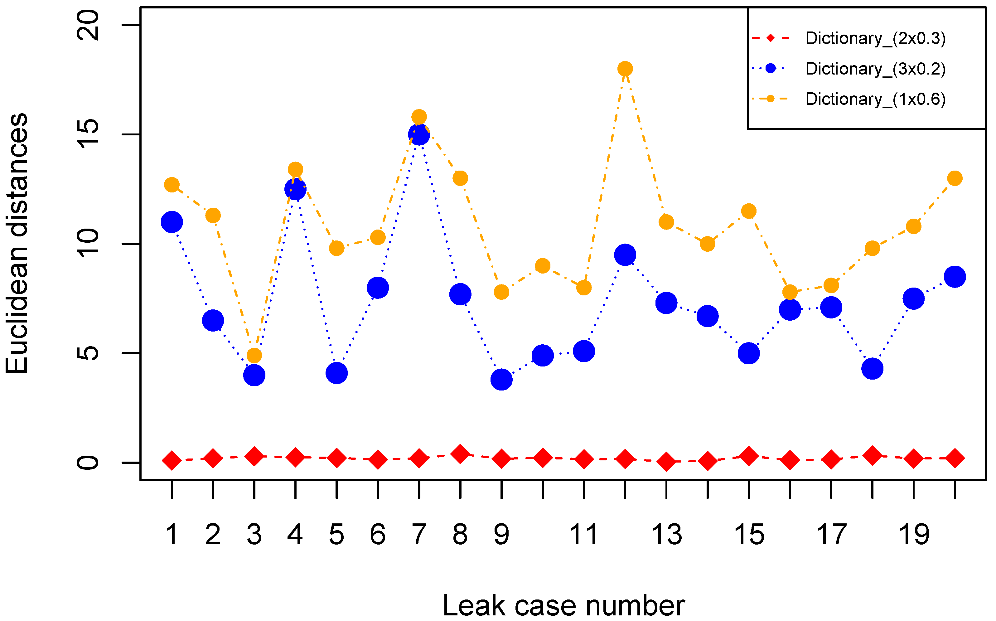
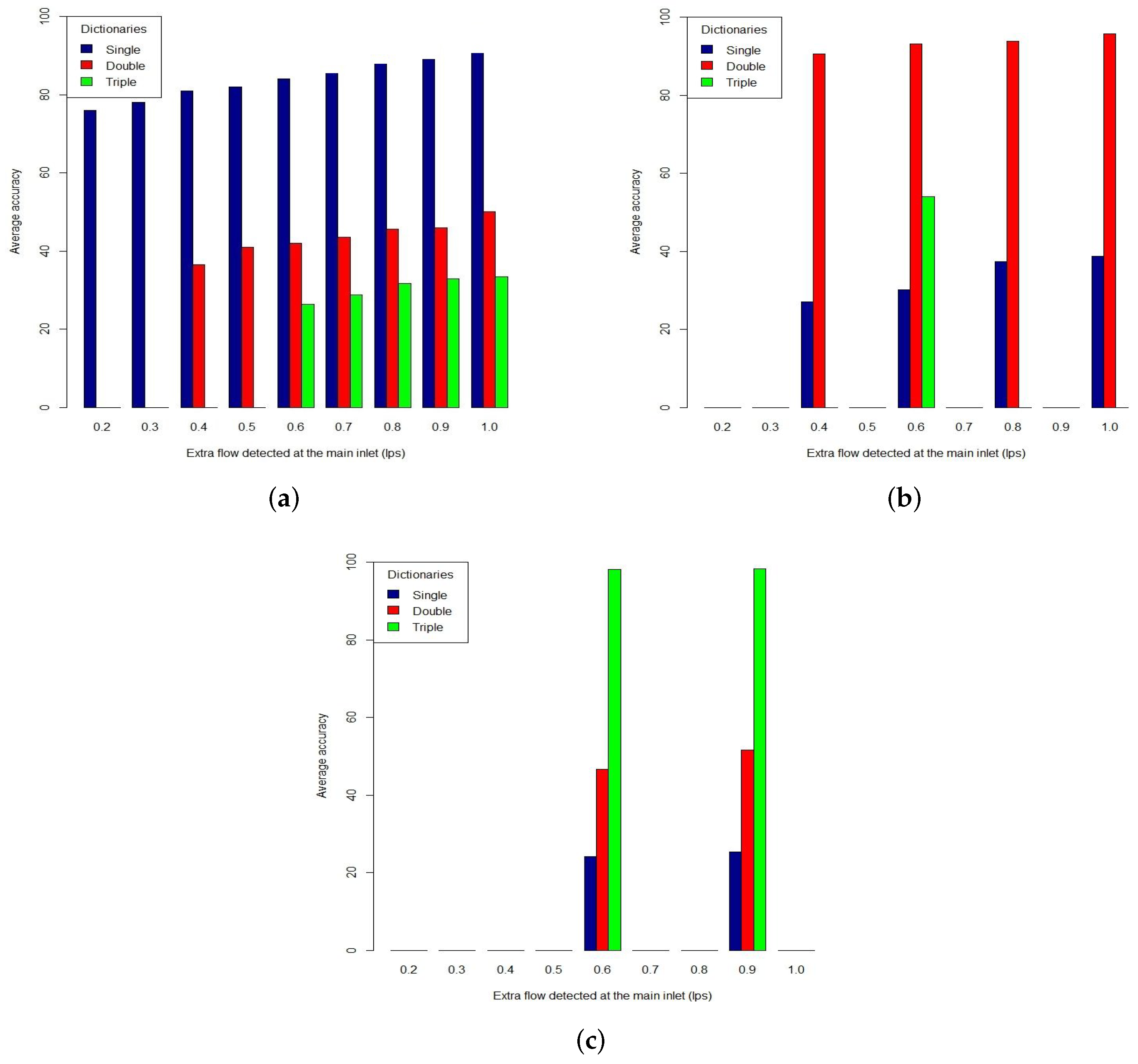
Vectors of the correct dictionary consistently result in the lowest Euclidean distances. For example, the lowest Euclidean distances to quantify double leaks are resulted from the vectors of a selected double leak dictionary (
Figure 4). This result shows that our method is accurate to distinguish different types of leaks. By applying the method, we calculated the averaged quantification accuracies of single, double and triple small leaks range from 70% to 85% (
Figure 5a–c). Smaller networks tend to produce higher quantification results due to the higher vector-to-junction ratio which indicates the distinctiveness of leak signatures in dictionaries. A dictionary vector of a small network commonly represents fewer junctions, hence, a higher vector-to-junction ratio. These results indicate that our method is effective in localizing single and multiple leaks.
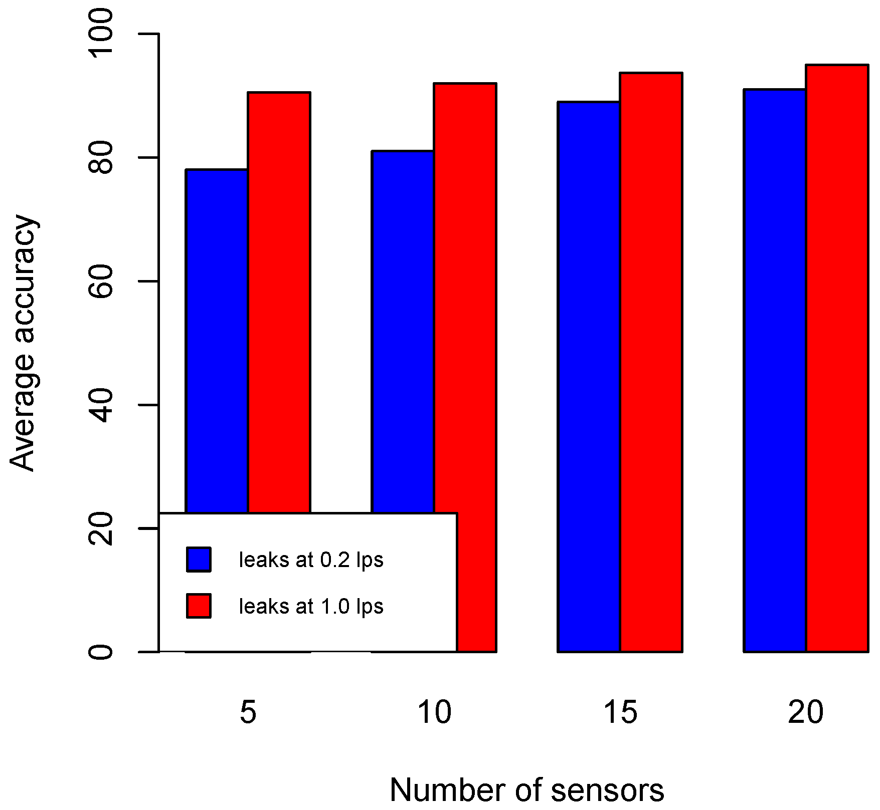
We extended our experiment by generating single, double and triple leaks within the range of [
] lps. We quantified the leaks by using corresponding dictionaries generated by using different numbers of sensors, that is,
. With five sensors, the performance of leak quantification has reached
at the lowest leak size (
lps) and
at highest leak size (1.0 lps). When more sensors are used, the performance gradually improves, especially in quantifying smaller sized leaks (
Figure 6). At some point, the improvement is insignificant. This is noticeable at the addition of 15 to 20 sensors. This shows that our method is effective in finding the locations of sensors which maximize their utility even with fewer sensors.
4.5. Comparisons
We compare our sensor placement strategy to the strategies that we consider as the state-of the art explained in
Section 2. First, we compare our method with the method developed by Narayanan et al. [
15] that used one sensor at the inlet of a WDN to find all leaks in it. Again, we used the Beckenham network to conduct our experiment due to its balanced complexity. We simulated leaks at 1.0 lps to examine the effectiveness of the method. Note that 1.0 lps leaks is the highest size of small leaks defined in Reference [
1]. The method [
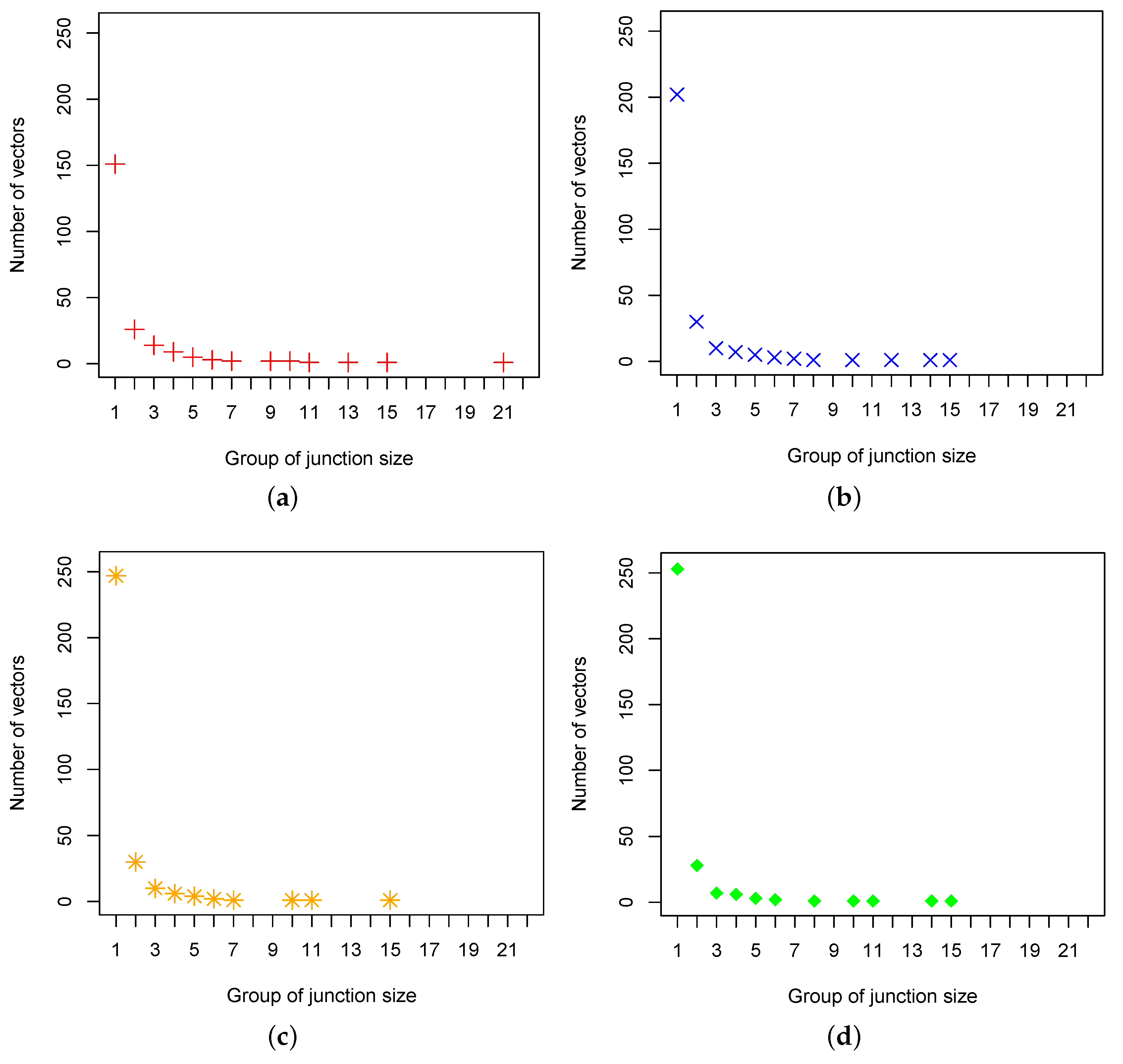
15] only recorded five leak signatures that quantify leaks into large group of junctions where each of them contains 157, 82, 81, 75, and 47 junctions. The leak signatures are fewer when the leaks are simulated at smaller sizes. This means the method produced low quantification certainty when applied for small leaks. Our method produced significant number of distinct leak signature that quantify leaks up to junction level (
Figure 7). The figure indicates that, with five sensors, there are 156 unique leak signatures that quantify one junction and there is only one unique leak signature that quantify a group of 21 junctions. The largest group of junctions quantified with five sensors is not even half of the smallest group of junctions quantified by the method in Reference [
15]. The number of leak signatures that quantify one junction increases along with the addition of sensors, while the number of leak signatures that quantify larger group of junctions decreases. This result shows that the method is not suitable to quantify small leaks despite the method is considered as the most efficient one in terms of the number of sensors used.
Second, we compare our method with the method developed by Sanz et al. that modeled demands based on their geographical locations [
16]. The method works similar to our cluster-based leak quantification method where locations that are geographically close tend to have similar leak signatures. The research used five sensors to examine its performance to localize leaks simulate at three different locations at a time (i.e., 1 lps, 3 lps and 5 lps) and three demand patterns. Thus, constituting nine scenarios in total. The accuracy of the localization was measured by the distance between the predicted leak location and the real one. The research in Reference [
16] examined the quantification performance by measuring the distance between a predicted leak location to the actual location of the leak. The research managed to quantify eight out of the nine scenarios with the average distance of predicted to the actual leak location by 370 m. Our method can be used to quantify single and multiple leaks at any position in a network. The use of five sensors produced 97% accuracy that quantify single leaks to the actual position. This result outperforms the method proposed in Reference [
16].
4.6. Subspace Voting Quantification
We conducted the subspace voting quantification experiments using n vectors generated at y lps leak size with s sensors. Suppose there are five sensors placed in pipes and in the Beckenham network. The sensors produced 72 unique vectors for leaks at 0.2 lps. All vectors along with their corresponding locations are stored in a dictionary of leak signatures at 0.2 lps (). To simulate a lps or a lps biased sensors, we perturb the vectors in the by adding or subtracting one or more columns of each vector by lps or lps.
There are 31 possible subspaces that can be generated from five sensors ( possible combinations). The subspaces are generated from one sensor location until the whole five sensor locations. For example, one column of a vector v of dictionary gets perturbed at with a lps bias. The vector becomes . To find the subspace votes, we calculate the Euclidean distances of every subspace of against the correlated subspace of each vector in . Whenever we find a subspace of a dictionary vector with the lowest distance () to the corresponding subspace of , we mark the vote of the dictionary vector with 1. We mark 0 if opposite. So, there are 31 (the number of possible subspaces) × 72 votes (the number of dictionary vectors) to quantify the perturbed vector . We perform the same method to obtain all possible perturbed vectors caused by a lps bias at . This procedure procedures 72 perturbed vectors.
Localizing the 72 perturbed vectors by using the subspace voting method produces higher performance compared to our naive quantification method (
Table 6). This result shows that the correctly functioning sensors can preserve the separation of leak signatures through the voting method. Quantification performances are higher for larger leak sizes due to the more extended separation of leak signatures. Thus, the effect of biased sensors can be minimized. This trend also applies to double and triple leak quantification. The other trend is that the subspace voting quantification method consistently outperforms the naive quantification method when more sensors are used. These results strengthen the evidence that the subspace voting quantification method is a better approach to mitigate biased sensors.
5. Discussion
Finding the MCL size of a WDN is a trial and error process by considering the limitation of the EPANET simulator, the common flow sensors specification and the size of a WDN. For example, EPANET can simulate flow up to four decimal digits, however, this detailed decimal number may not be feasible for sensors to read. We limit the EPANET flow simulation to a maximum of two decimal digits where recent manufactured sensors can read. Then, finding the trial and error process to find MCL is performed from the smallest possible leaks defined in Reference [
1]. Smaller MCL (e.g., 0.1 lps to 0.2 lps) can be simulated in smaller-sized WDNs with low average connection degree (<= 2.5), while larger -sized WDNs with high average connection degree (> 2.5) require higher MCL (e.g., >= 0.3 lps) to generate lean graphs for every possible leak locations.
Quantifying small leaks can be performed by elaborating sensors placed at the most strategic locations in a water distribution network. One compulsory location where a sensor to be placed is the inlet of a WDN. The sensor located at the WDN inlet not only detects the presence and the size of a leak in the WDN, but also locates the leak in a WDN with multiple tanks or reservoirs (e.g., the Pescara network [
27]). This quantification method is feasible to use due to the fact that leaks attract more extra flows from the closest tank or reservoir. By only utilizing sensors placed at the inlets of a multi-tank WDN, we can partition the WDN into clusters based on the source tank of extra flows. To increase the depth of the quantification, additional sensors can be placed using our proposed sensor placement strategy.
Our proposed leak signature dictionary to quantify leaks is effective when the number of sensors is sufficient to cover a network. For example, five sensors can produce finer leak quantification (up to the junction level) because the leak signatures are quite distinct. However, for larger-sized networks, the five sensors might not be able to reach the level due to less distinctive leak signatures. In this case, finding the actual leak location must be performed manually, for example, using an acoustic sensor in an area whose leak signature has the closest euclidean distance with an observed flow readings. This situation can lead to the increase of the uncertainty to find the actual leak location in a network with higher average connection degree.
The experimental results on the single and multiple leak quantification have indicated that our method has promising results (
Figure 5). Our method is significantly different from what we consider as the most advanced method that only requires one flow sensor to quantify leaks proposed in Reference [
15] and a similar method to ours that quantify leaks in clusters based on their geographical locations [
16]. However, there are some conditions for our method to work properly. First, we assume flows are steady in a snapshot of the MNF. Then, we use the snapshot to simulate leaks at every possible location in a WDN to generate the lean graphs. In reality, this condition might not be the case due to sensor inaccuracies or an altered pattern of water usage. Second, EPANET can tolerate up to 0.001 inaccuracy to run the hydraulic equations. This characteristic also influences our experiments.
The drawback of the subspace voting quantification is that it requires an exhaustive computation as the vote must be conducted for all possible subspaces. To illustrate the computation, with the five sensors, a biased sensor in results in 72 perturbed vectors. To quantify the leak vectors, it requires 72 (perturbed vectors) × 72 (dictionary vectors) × 31 (all possible subspaces) = 160,704 calculations. This number grows significantly when we simulate two or three possible biased sensors. The number of calculations is 160,704 × 25 (5 possible locations for single bias sensor + 10 possible locations for two bias sensor and + 10 possible locations for three bias sensor) = 4,017,600 computations. The computations grow as more sensors are used. Despite the huge number of computations, this is the most common sense approach to implement given the lack of knowledge which sensors are biased and which sensors are functioning correctly.
6. Conclusions
We have shown that our sensor placement strategy is effective at quantifying single and multiple small leaks. Experimental results proved that our sensor placement strategy is robust when applied in WDNs with a various features. Our sensor placement strategy is also flexible in accommodating cost-sensitive locations while maintaining its performance. Lastly, we have shown that we can maintain the quantification performance when some sensors are biased using the subspace voting mechanism. As our experiments are purely based on simulations, we are intended to extend our experiments to use real water distribution networks to strengthen our hypothesis.
Author Contributions
Conceptualization, A.M.S. and R.C.-O.; Data curation, A.M.S.; Funding acquisition, R.C.-O.; Investigation, A.M.S.; Methodology, A.M.S., R.C.-O. and A.D.; Software, A.M.S.; Supervision, R.C.-O. and A.D.; Writing—original draft, A.M.S.; Writing—review & editing, R.C.-O. and A.D. All authors have read and agreed to the published version of the manuscript.
Funding
This research is funded by a grant from the Indonesian Directorate General of Higher Education (DIKTI) and CRC for Water Sensitive Cities sub project C5-1 Intelligent Urban Water Systems.
Conflicts of Interest
The authors declare that there is no conflict of interest in this work.
References
- Frauendorfer, R.; Liemberger, R. The Issues and Challenges of Reducing Non-Revenue Water. Asian Development Bank. 2010. Available online: http://hdl.handle.net/11540/1003 (accessed on 22 November 2020).
- Rossman, L.A. EPANET 2: Users Manual; U.S. Environmental Protection Agency: Cincinnati, OH, USA, 2000.
- Lin, C.-C.; Yeh, H.-D. An Inverse Transient-Based Optimization Approach to Fault Examination in Water Distribution Networks. Water 2019, 11, 1154. [Google Scholar] [CrossRef]
- Pudar, R.S.; Liggett, J.A. Leaks in pipe networks. J. Hydraul. Eng. 1992, 118, 1031–1046. [Google Scholar] [CrossRef]
- Jiawei, H.; Kamber, M.; Pei, J. Data Mining (Third Edition). The Morgan Kaufmann Series in Data Management Systems; Morgan Kaufmann: Boston, MA, USA, 2012. [Google Scholar]
- Vitkovsky, J.P.; Simpson, A.R.; Lambert, M.F. Leak detection and calibration using transients and genetic algorithms. J. Water Resour. Plan. Manag. 2000, 126, 262–265. [Google Scholar] [CrossRef]
- Wu, Z.Y.; Sage, P. Water Loss Detection via Genetic Algorithm Optimization-Based Model Calibration. Water Distrib. Syst. Anal. Symp. 2006, 247, 180. [Google Scholar]
- Mamo, T.G. Virtual DMA Municipal Water Supply Pipeline Leak Detection and Classification Using Advance Pattern Recognizer Multi-Class SVM. J. Pattern Recognit. Res. 2014, 1, 25–42. [Google Scholar] [CrossRef]
- Barradas, I.; Garza, L.E.; Morales-Menendez, R.; Vargas-Martínez, A. Leaks Detection in a Pipeline Using Artificial Neural Networks; Lecture Notes in Computer Science (Including Subseries Lecture Notes in Artificial Intelligence and Lecture Notes in Bioinformatics); Springer: Berlin/Heidelberg, Germany, 2009; Volume 5856, pp. 637–644. [Google Scholar]
- Sun, C.; Parellada, B.; Puig, V.; Cembrano, G. Leak localization in water distribution networks using pressure and data-driven classifier approach. Water 2020, 12, 54. [Google Scholar] [CrossRef]
- Cardell-Oliver, R.; Scott, V.; Chapman, T.; Morgan, J.; Simpson, A. Designing sensor networks for leak detection in water pipeline systems. In Proceedings of the 2015 IEEE Eighth International Conference on Intelligent Sensors, Sensor Networks and Information Processing (IEEE ISSNIP 2015), Singapore, 7–9 April 2015. [Google Scholar]
- Abbas, W.; Perelman, L.S.; Amin, S.; Koutsoukos, X. An efficient approach to fault identification in urban water networks using multi-level sensing. In Proceedings of the 2nd ACM International Conference on Embedded Systems for Energy-Efficient Built Environments, BuildSys ’15, Seoul, Korea, 4–5 November 2015; pp. 147–156. [Google Scholar]
- Casillas, M.V.; Puig, V.; Garza-Castañón, L.E.; Rosich, A. Optimal sensor placement for leak location in water distribution networks using genetic algorithms. Sensors 2013, 13, 14984–15005. [Google Scholar] [CrossRef] [PubMed]
- Sarrate, R.; Nejjari, F.; Rosich, A. Sensor placement for fault diagnosis performance maximization in distribution networks. In Proceedings of the 20th Mediterranean Conference on Control & Automation (MED), Barcelona, Spain, 3–6 July 2012; pp. 110–115. [Google Scholar]
- Narayanan, I.; Vasan, A.; Sarangan, V.; Sivasubramaniam, A. One meter to find them all-water network leak localization using a single flow meter. In Proceedings of the 13th International Symposium on Information Processing in Sensor Networks, Berlin, Germany, 15–17 April 2014; pp. 47–58. [Google Scholar]
- Sanz, G.; Perez, R.; Kapelan, Z.; Savic, D. Leak detection and localization through demand components calibration. J. Water Resour. Plan. Manag. 2016, 142, 04015057. [Google Scholar] [CrossRef]
- Lucas, M.W. Network Flow Analysis, 2nd ed.; No Starch Press Inc.: San Fransisco, CA, USA, 2010. [Google Scholar]
- De Silva, D.; Mashford, J.; Burn, S. Computer Aided Leak Location and Sizing in Pipe Networks, 2nd ed.; Urban Water Security Research Alliance City East, Qld: Alliance, OH, USA, 2011. [Google Scholar]
- Russell, S.; Norvig, P. Artificial Intelligence: A Modern Approach; CreateSpace Independent Publishing Platform: Scotts Valley, CA, USA, 2016. [Google Scholar]
- Russell, J.; Cohn, R. Bisection Method; Book on Demand; 2012; ISBN1 5512717871, ISBN2 9785512717875. Available online: https://books.google.com.au/books?id=IcucMQEACAAJ (accessed on 18 November 2020).
- Kernighan, B.W.; Lin, S. An efficient heuristic procedure for partitioning graphs. Bell Syst. Tech. J. 1970, 49, 291–307. [Google Scholar] [CrossRef]
- Elhay, S.; Deuerlein, J.; Piller, O.; Simpson, A.R. Graph partitioning in the analysis of pressure dependent water distribution systems. J. Water Resour. Plan. Manag. 2018, 144, 04018011. [Google Scholar] [CrossRef]
- Rajeswaran, A.; Narasimhan, S.; Narasimhan, S. A graph partitioning algorithm for leak detection in water distribution networks. Comput. Chem. Eng. 2018, 108, 11–23. [Google Scholar] [CrossRef]
- Levandowsky, M.; Winter, D. Distance between sets. Nature 1971, 234, 34–35. [Google Scholar] [CrossRef]
- Clark Solutions. 7000/8000 Series Flow Meter With Optional Outputs; Technical Report; Clark Solutions: Hudson, MA, USA.
- Tolson, B.A.; Khedr, A. Battle of Background Leakage Assessment for Water Networks (BBLAWN): An Incremental Savings Approach. Procedia Eng. 2014, 89, 69–77. [Google Scholar] [CrossRef]
- Department of Homeland Security. Water Distribution System Research Database. Kentucky Critical Infrastructure Protection Program, under OTA No HSHQDC-07-3-00005, Subcontract No 02-10-UK; Department of Homeland Security: Washington, DC, USA, 2016. [Google Scholar]
- Water Corporation of Western Australia. Water Distribution Network Research Database; WA Water Corporation Research Center: Osborne Park, WA, USA, 2017. [Google Scholar]
- Krause, A.; Leskovec, J.; Guestrin, C.; VanBriesen, J.; Faloutsos, C. Efficient sensor placement optimization for securing large water distribution networks. J. Water Resour. Plan. Manag. 2008, 134, 516–526. [Google Scholar] [CrossRef]
- Zhao, W.; Beach, T.H.; Rezgui, Y. Optimization of potable water distribution and wastewater collection networks: A systematic review and future research directions. IEEE Trans. Syst. Man Cybern. Syst. 2016, 46, 659–681. [Google Scholar] [CrossRef]
- Carnevali, L.; Tarani, F.; Vicario, E. Performability evaluation of water distribution systems during maintenance procedures. IEEE Trans. Syst. Man Cybern. Syst. 2020, 50, 1704–1720. [Google Scholar] [CrossRef]
| Publisher’s Note: MDPI stays neutral with regard to jurisdictional claims in published maps and institutional affiliations. |
© 2020 by the authors. Licensee MDPI, Basel, Switzerland. This article is an open access article distributed under the terms and conditions of the Creative Commons Attribution (CC BY) license (http://creativecommons.org/licenses/by/4.0/).


