Article

Hybridised Artificial Neural Network Model with Slime Mould Algorithm: A Novel Methodology for Prediction of Urban Stochastic Water Demand

by
Salah L. Zubaidi
1,*,
Iqbal H. Abdulkareem
2,
Khalid S. Hashim
3,4,
Hussein Al-Bugharbee
5,
Hussein Mohammed Ridha
6,
Sadik Kamel Gharghan
7,
Fuod F. Al-Qaim
8,
Magomed Muradov
3,
Patryk Kot
3 and
Rafid Al-Khaddar
3
1
Department of Civil Engineering, Wasit University, Wasit 52001, Iraq
2
Environmental Research and Studies Centre, University of Babylon, Babylon 51001, Iraq
3
BEST Research Institute, Liverpool John Moores University, Liverpool L3 3AF, UK
4
Department of Environment Engineering, University of Babylon, Babylon 51001, Iraq
5
Department of Mechanical Engineering, Wasit University, Wasit 52001, Iraq
6
Department of Electrical and Electronics Engineering, Faculty of Engineering, Universiti Putra Malaysia, Serdang 43400, Malaysia
7
Department of Medical Instrumentation Techniques Engineering, Electrical Engineering Technical College Middle Technical University, Al Doura, Baghdad 10022, Iraq
8
Faculty of Science for Women, Babylon University, Babylon 51001, Iraq
*
Author to whom correspondence should be addressed.
Water 2020, 12(10), 2692; https://doi.org/10.3390/w12102692
Submission received: 26 July 2020 / Revised: 20 September 2020 / Accepted: 24 September 2020 / Published: 26 September 2020
(This article belongs to the Special Issue Advanced Applications of Electrocoagulation in Water and Wastewater)

Abstract

:
Urban water demand prediction based on climate change is always challenging for water utilities because of the uncertainty that results from a sudden rise in water demand due to stochastic patterns of climatic factors. For this purpose, a novel combined methodology including, firstly, data pre-processing techniques were employed to decompose the time series of water and climatic factors by using empirical mode decomposition and identifying the best model input via tolerance to avoid multi-collinearity. Second, the artificial neural network (ANN) model was optimised by an up-to-date slime mould algorithm (SMA-ANN) to predict the medium term of the stochastic signal of monthly urban water demand. Ten climatic factors over 16 years were used to simulate the stochastic signal of water demand. The results reveal that SMA outperforms a multi-verse optimiser and backtracking search algorithm based on error scale. The performance of the hybrid model SMA-ANN is better than ANN (stand-alone) based on the range of statistical criteria. Generally, this methodology yields accurate results with a coefficient of determination of 0.9 and a mean absolute relative error of 0.001. This study can assist local water managers to efficiently manage the present water system and plan extensions to accommodate the increasing water demand.

1. Introduction

Security of municipal water is fundamental to gain a sustainable environment in modern cities, especially under the impact of global warming and socio-economic variables. Additionally, most cities are located close to freshwater sources to ensure the prosperity of both industry and agriculture. For the mentioned reasons, freshwater scarcity is a classic problem for policymakers [1,2]. Recently, the World Economic Forum confirmed that water scarcity is one of the largest international risks because of the limited amount of accessible freshwater (approximately 0.014% of the total amount of water on Earth). In addition, climate change, water pollution and poor management of freshwater sources are other major factors that contribute to water scarcity. For example, climate change increases water demand which increases the pressure on the urban water system, especially during periods of water shortage. Accordingly, water companies must devise strategies to tackle this issue. Hence, water utilities should support and enhance the management of the municipal water system [3,4,5].
Hemati et al. [6] reported that, during the period from 1930 to 2009, Melbourne experienced two short-term droughts and three long-term droughts (the last one was from 1997 to 2009). As a result, annual rainfall was adversely affected, making its influence on the municipal water supply system keenly felt. In addition, Roy and Majumder [7] stated that hazardous weather events, such as heatwaves in Australia, are likely to be more regular or extreme, leading to alterations in the amount of freshwater available.
In the last few decades, there has been a surge of interest in the effects of climate change on the demand for freshwater. Although data from several sources have identified that the increase of urban water demand is associated with climatic factors, researchers have not looked at the variability of climate change in much detail. Therefore, to date, the impact of climate change on urban water demand has still not yet been extensively investigated. Consequently, the uncertainty in water sustainability has increased due to the lack of knowledge about the impact of climate change on the demand of water [8].
Prediction of municipal water demand is crucial to manage, operate and plan urban water systems. It leads to a balance between water need and delivery, especially with the fluctuations caused by climate change that cause unexpected growth in water demand, fluctuations in stochastic patterns and an increase in the uncertainty for water utilities. Additionally, estimating water demand is quite useful for proper management, operation and upgrading of present freshwater sources [8,9,10]. Ebrahim Banihabib and Mousavi-Mirkalaei [11] stated that modelling techniques for prediction of municipal water demand are required to address the potential water security. Prediction of medium-term water demand is classified as a tactical type, and it is used to improve water supply networks and installations and to manage dam reservoirs [12].
A review of different municipal water demand modelling techniques over the past few decades [5,13,14,15,16] highlighted various issues that include: (1) Most of these methods and techniques were focused on the prediction of short-term water demand, and little research has considered medium- to long-term urban water demand; (2) different artificial intelligence techniques were successfully applied to simulate urban water demand, such as artificial neural network [8], support vector regression [17], adaptive neuro-fuzzy inference system [18] and random forests [19]; (3) several studies indicated that hybrid techniques yield superior outcomes when compared with the classical single models, such as Chen et al. [19] and Altunkaynak and Nigussie [20]; and (4) a number of methods, techniques and models have been used to forecast water demand based on weather or climatic factors. However, these techniques have been largely deterministic and focus generally on only a few weather variables, such as the study of Mouatadid and Adamowski [21]. Very limited research has used the stochastic signal to predict water demand based on climatic factors, such as the studies of Zubaidi et al. [22] and Zubaidi et al. [8]. These studies used the stochastic model to predict the stochastic signal of water demand of an area in Melbourne that served by the Yarra Valley Water utility, considering the effects of five climatic factors, and applied two hybrid models (particle swarm optimisation and artificial neural network (PSO-ANN)) and lightning search algorithm and artificial neural network (LSA-ANN).
Although the application of machine learning and data analytic methodologies in urban water estimating have grown considerably in recent years, more investigations are needed to develop new methodologies to enhance the results from present conservation and demand management programmes [5]. Altunkaynak and Nigussie [9] stated that the artificial neural network is a preferred option to simulate water demand because it can deal with non-linear time series.
Different metaheuristic optimisation algorithms could be applied to tackle a range of problems for various application domains. The main advantages of optimisation algorithms are their ability to select the optimal values of parameters of the system under different conditions, and they have time-saving qualities. Recently, a multi-verse optimiser (MVO) proposed by Mirjalili et al. [23] to solve various optimisation problems, for example, has been used for energy management in smart cities [24] and multi-level image segmentation [25]. Additionally, a backtracking search algorithm (BSA) has been utilised to tackle several optimisation issues, such as predicting urban water demand depending on previous water consumption data [26], photovoltaic models [27] and power signals [28]. Moreover, a slime mould algorithm (SMA) has been proposed by Li et al. [29] and used in several optimisation issues, but has not been investigated in the urban water sector, such as the spring design problem [30], photovoltaic models [31] and image segmentation method [32].
In addition, the literature has emphasised the importance of using data pre-processing to improve the quality of time series and to determine the best independent variables. More attention has recently focused on data cleaning. Therefore, several signal pre-treatment techniques have been employed to clean and/or detect the trend, seasonal and stochastic components of water consumption time series, such as singular spectrum analysis (SSA) [33,34], wavelet transform (WT) [20,35], variational mode decomposition (VMD) [36] and empirical mode decomposition (EMD) [37,38]. Another significant aspect of data pre-processing is selecting the best independent variables, such as principal component analysis (PCA) [39,40], mutual information (MI) [41,42] and variance inflation factor (VIF) [22,43].
Despite the fact that different techniques and approaches were used to forecast the future water demand, water companies still face challenges in estimating the accurate water demand, especially with the influence of climatic factors and their implications for future water demand. Therefore, additional research studies are required to accurately estimate the growing water demand [8].
In this context, the main contributions of the current research are:
  • The employment of 10 climatic factors over 16 years to assess the impact of climate change on urban water demand.
  • Development and analysis of a new hybrid algorithm SMA-ANN for the water demand optimisation problem, and choosing the optimal hyperparameters of the ANN approach.
  • The application of two hybrid algorithms, MVO-ANN and BSA-ANN, for analysing and validating the proposed SMA-ANN algorithm.
  • Using the novel methodology, which contains data pre-processing techniques (EMD and tolerance) and hybrid SMA-ANN algorithm, to simulate the monthly stochastic pattern of water demand based on the best scenario of climatic factors over 16 years.
  • Minimising the uncertainty by applying three metaheuristic algorithms for more validation, and using the ANN (stand-alone) to confirm the results of the SMA-ANN model. Additionally, employing 10 climatic factors that give scientific insight (i.e., to what extent climate change has driven water demand) for policymakers to achieve sustainability.
To the best of the authors’ knowledge, the present study explores a novel methodology for the first time: the effects of climate change on the monthly stochastic pattern of urban water demand. The structure of the research is organised as follows: case study and data used are presented in Section 2; the proposed methodology for predicting monthly stochastic water demand is described in Section 3; Section 4 provides the analysis and compares the obtained results; and finally, Section 5 presents the final conclusions with some considerations of the study.

2. Case Study and Data Used

The suggested methodology was applied to the observed water consumption and climatic factor data relating to the South East Water (SEW) utility, which is one of three retail water utilities that purchase water wholesale from the Melbourne Water company in Melbourne, Australia. The sources of freshwater are 11 large storage facilities, which are refilled regularly by stormwater harvesting [44]. The urban water system network of SEW utility serves more than 1.7 million individuals in a 3640 km2 area, and the company has approximately 72,700 customers, categorised into residential, industrial and commercial [45].
The collected data comprise monthly urban water consumption (megalitre, ML), maximum temperature (Tmax) (°C), minimum temperature (Tmin) (°C), mean temperature (Tmean) (°C), solar radiation (Srad) (MJ/m2), potential evapotranspiration (FA-O56) (mm), vapour pressure (VP) (hpa), rainfall (Rain) (mm), evaporation (Eva) (mm), maximum relative humidity (RHmax) (%) and minimum relative humidity (RHmin) (%) from 2000 to 2015. Figure 1 shows the time series and box plot of monthly water consumption for SEW utility. The figure reveals the decrease in water consumption due to drought, and water-conserving policies and initiatives. After that, the consumption increased, possibly because restrictions were eased after the impact of the drought lessened. It may also be due to the strategies that Melbourne Corporation pursued by upgrading the dams and relying on other resources, such as water desalination and water recycling [44].

3. Proposed Methodology

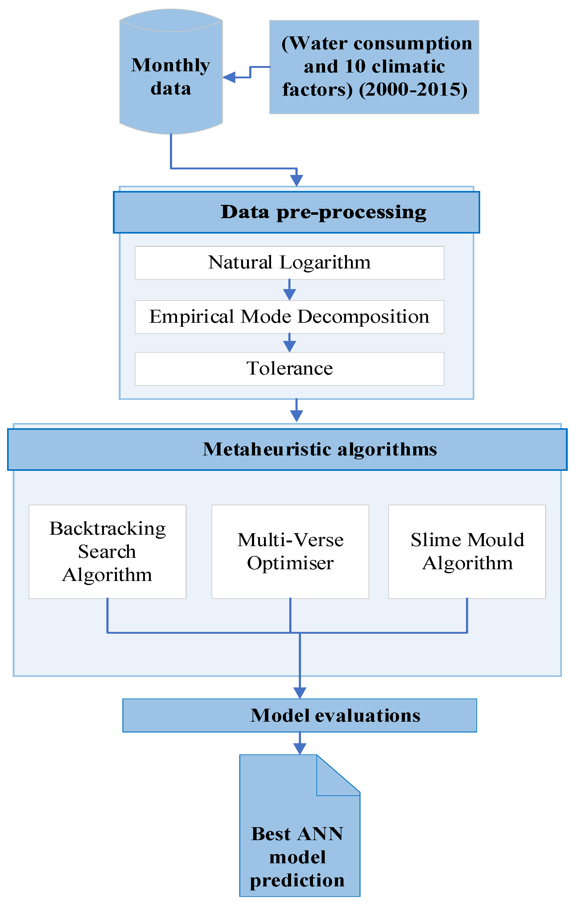
There is a relatively small body of literature that is concerned with the impact of climate change only on the municipal water demand. Accordingly, this paper proposes a novel combined methodology for investigating the impact of climate change on water demand. It could be divided into five main categories: data pre-processing, slime mould algorithm (SMA), artificial neural network (ANN), hybrid metaheuristic algorithm-based artificial neural network and model evaluation. Figure 2 shows the structure of the proposed methodology to predict monthly stochastic data of water demand based on climatic factors.

3.1. Data Pre-Processing

Recent developments in urban water predictive methodologies have highlighted the need to apply different data pre-processing techniques, which could be classified into normalisation, cleaning and selection of best model input [5,46]. To be in accordance with Tabachnick and Fidell [47], the natural logarithm was used to normalise all raw time series of water and climatic factors to reduce both the impact of the outliers and the multi-collinearity between independent factors.
Zubaidi et al. [8] mention that the relation between water demand time series and climatic time series is stochastic. Stochastic models will also offer a better reflection of reality and insight into the system’s dynamics [48]. Hence, an empirical mode decomposition (EMD) approach was applied to decompose the original time series of dependent and independent variables into trend, seasonal, stochastic and noise components, and to detect the stochastic component after that. EMD is used in the analysis of various problems, such as machinery fault diagnosis [49] and biomedical signal analysis [50].
EMD is also used for analysing geodetic data [51]. In this study, the authors have used EMD to analyse the natural variability of sea level and its effect, among other factors, on the trend of the sea level. Recently, Chu and Huang [52] utilised EMD for synthetisation and generation of flow data and for increasing the number of flow time series for the same time period, which is used in the simulation of a water supply system. This technique decomposes a time series into a number of time domain components called intrinsic mode functions (IMFs). The latter must have two properties:
  • The maximum difference between the number of local maxima and minima is one.
  • The mean value of an IMF is zero.
For a time series x(t), the extraction of IMFs could be described briefly in the following steps [51]:
  • Assume hk − 1(t) = x(t), and hi,k − 1(t) = x(t), where i and k refer to the IMF number and the iteration number for finding the accurate ith IMF, respectively.
  • Identify all the maxima and minima points of the series hi,k − 1(t).
  • Connect the maxima points by cubic spline interpolation and do the same thing for the minima points. The linked maxima points are called the upper envelope, Ui,k − 1(t), while the linked minima points are called the lower envelope, Li,k − 1(t).
  • The mean of the upper and lower envelopes is found using this formula: mi,k − 1(t) = (Ui,k − 1(t) − Li,k − 1(t))/2.
  • Form the following formula: hi,k(t): = hi,k − 1(t) − mi,k − 1(t). The component hi,k(t) is primarily described as the first IMF. To determine the first IMF accurately, the hi,k(t) is considered as a new signal, and the mean of upper envelope, lower envelope and the mean (i.e., UI,k(t), Li,k − 1(t) and mi,k of the hi,k(t)) are calculated. The new component hi,k(t) is checked to see whether it has IMF properties or not. If it does, then it (i.e., hk(t)) is identified as an IMF. If not, the process will be repeated until IMF properties are obtained. The number of the repetitions to identify an IMF is called iterations and is notated by k, while the IMF number is notated by i.
  • When the ith IMF is obtained, the residue is obtained: resi = hi,k − 1 − IMFi.
  • The residue resi is now treated as the signal hi+1,k − 1 and the same steps 2–6 are repeated until no more IMFs can be extracted.
The EDM process above is applied for all dependent and independent variables in this study.
Regarding the selection of the best model input, Pallant [52] recommended using a tolerance method to choose the independent variables that have a tolerance value of more than 0.1, because values less than 0.1 indicate the presence of multi-collinearity.

3.2. Slime Mould Algorithm (SMA)

The SMA is one of the recent nature-inspired algorithms. It refers to the mathematical model of simulating the propagation wave of slime mould when forming the optimal path for connecting foods. This model adaptively simulates the process of producing negative and positive feedback during the propagation wave. This algorithm is incorporated into different optimisation problems, including the engineering ones. The main two stages in the SMA algorithm are called approaching food and warp food.
a.
Approaching food
In this stage, the slime is approaching food based on its odour in the air, and this behaviour is mathematically described as follows:
X ( t + 1 ) = { X b ( t ) + vb × ( W × X A ( t ) X B ( t ) ) ,   r < p vc × X ( t ) ,   r p
where
vb is a parameter which ranges from −a to a.
vc   represents a parameter which decreases from one to zero in a linear form.
Xb represents the current individual location corresponding to high odour concentration.
t is the current iteration.
X is the location of the slime mould.
X A   and   X B are randomly selected individuals from the mould.
W is the weight of the slime mould.
The formula of p can be represented as follows:
p = tanh [ S ( i ) DF ]   where   i ϵ   1 , 2 , 3 , ,   n
S(i) represents the fitness of X .
DF represents the best fitness over all the iterations.
As mentioned above, vb   ranges from −a to a, and a can be described as follows:
a = arctanh ( ( t max t ) + 1 )
The W formula can be described as follows:
W ( SmeelIndex ( t ) ) ¯ = { 1 + r × log ( bF S ( i ) bF wF + 1 ) ,             condition 1 r × log ( bF S ( i ) bF wF + 1 ) ,       others
SmeelIndex = sort ( S )
where
r denotes the random value within the interval [0, 1].
bF represents the optimal fitness obtained in the current iterative process.
wF represents the worst fitness value obtained in the current iterative process.
SmeelIndex refers to the sequence of fitness values.
b.
Warp food
In this stage, the behaviour of the slime in conducting contraction of its venous structure is mathematically described as follows.
X * = { rand × ( UB LB ) + LB , rand < z X ( t ) + vb × (   W   × X A ( t ) X B ( t ) ) ,   r < p vc × X ( t ) ,   r p
where LB and UB are the lower and upper boundaries of the search range, and rand and r are random parameters ranging from 0 to 1. Further details of the SMA can be found in Li et al. [29]. In this study, the SMA algorithm is combined with the ANN model to determine the optimum parameters of the ANN model (see Section 3.4).

3.3. Artificial Neural Network (ANN)

In recent years, there has been an increasing interest in using the ANN model to predict urban water demand, because it is capable of accurately simulating the nonlinear time series. Additionally, Rahim et al. [5] reported that different multi-layer feedforward neural networks (MLFFNNs) have been successfully developed utilising propagation networks in a water demand estimation model for short and medium terms. The Levenberg–Marquardt (LM) backpropagation algorithm was employed for training the ANN model because it can effectively simulate any independent/dependent map [53]. The structure of the ANN model can be categorised into four layers: the input layer, two hidden layers and an output layer. The input layer contains the independent variable (climatic factors), the output layer involves the dependent variable (water demand) and the hidden layers comprise the hidden neurons, which are responsible for stimulating the nonlinear relationship between water consumption and climatic factors. As in Zubaidi et al. [43], the tansigmoidal activation function was considered in both of the hidden layers and the linear activation function was utilised in the output layer. In this research, total data can be randomly categorised into training (70%), testing (15%) and validation datasets (15%) [54]. Following González Perea et al. [55], the ANN model was integrated with a metaheuristic algorithm to determine the optimal hyperparameters of the ANN model that includes the learning rate coefficient (LR) and the number of neurons hidden in the first (N1) and second (N2) hidden layers.

3.4. Hybrid Metaheuristic Algorithm-Based Artificial Neural Network

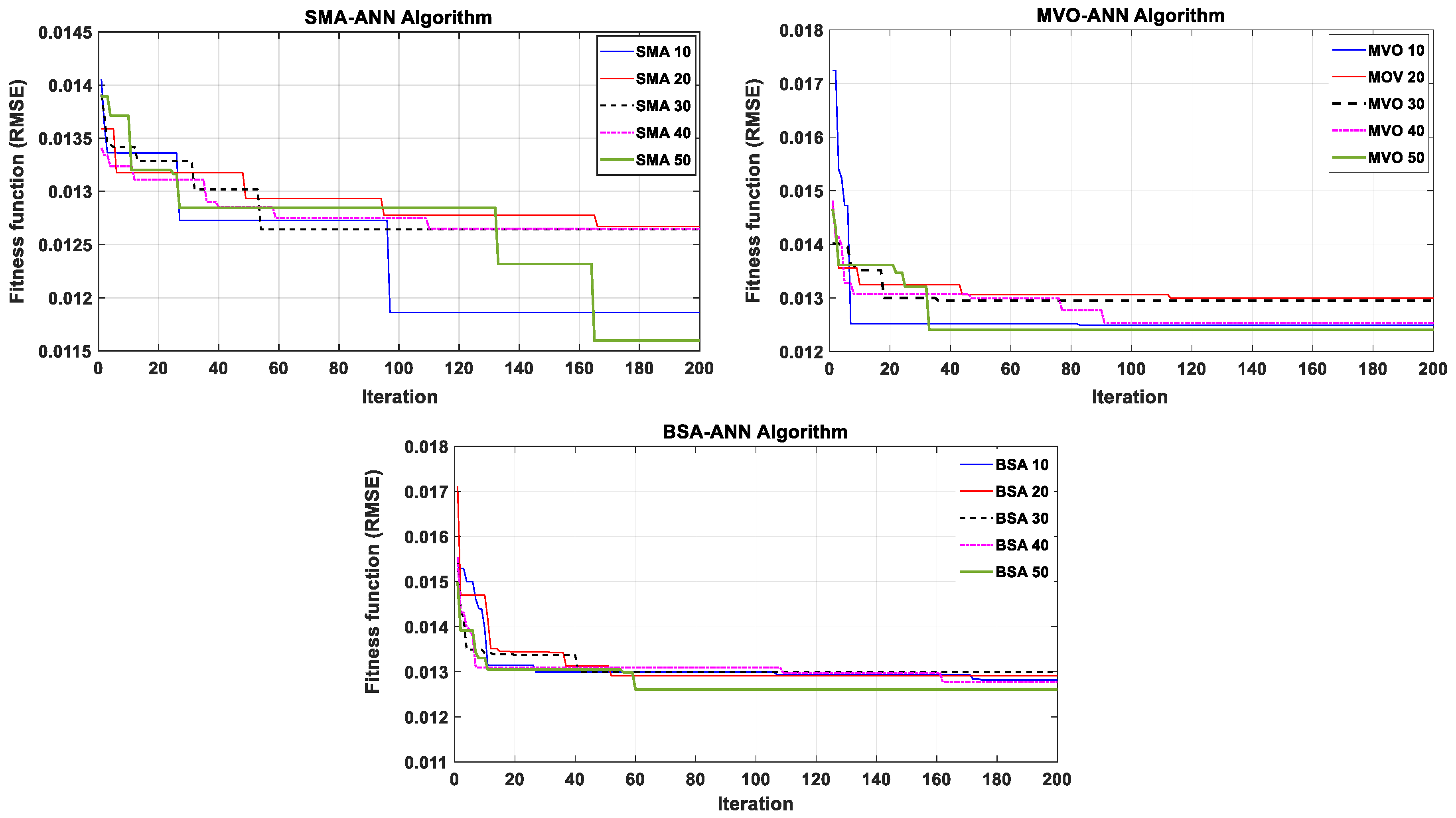
In the ANN technique, before achieving the stages of training, testing and validation, it is important to locate two hyperparameters, which are the learning rate coefficient (LR) and the number of neurons hidden (N1 and N2) for the hidden layer one and two, respectively. These hyperparameters are responsible for mapping the nonlinear relationship among the stochastic signals of water consumption and climatic factors. The determination of these hyperparameters, based on a trial and error procedure, may not present the optimum solutions. For this purpose, the ANN model is hybridised with the slime mould algorithm (SMA-ANN) (automated machine learning) to select the best LR, N1 and N2 for the ANN model. Additionally, two extra metaheuristics were hybridised with the ANN, the multi-verse optimiser (MVO-ANN) and the backtracking search algorithm (BSA-ANN), to assess and validate the results of the SMA-ANN algorithm. Five population sizes (10, 20, 30, 40 and 50 popsize) with 200 iterations were employed for each hybrid algorithm to select the popsize that could offer the lower value of fitness function (root mean square error, RMSE).

3.5. Model Evaluation

In this research, several performance statistical criteria were employed to evaluate the performance of the suggested methodology, because there are no global performance criteria that are appropriate for a particular usage. The performance criteria employed in this research are categorised into absolute, relative and dimensionless errors [36]. The absolute error contains the mean absolute error (MAE, Equation (7)) and mean square error (MSE, Equation (8)). The relative error comprises the mean absolute relative error (MARE, Equation (9)). The dimensionless error contains the coefficient of determination (R2, Equation (10)). In addition, a Bland–Altman scatterplot is used to graphically represent the upper and lower limits of agreement area between (actual data–simulated data) on the y-axis, and ((actual data + simulated data)/2) on the x-axis. Moreover, Augmented Dickey–Fuller (ADF) and Kwiatkowski–Phillips–Schmidt–Shin (KPSS) tests are used to examine the stationarity of the stochastic component for dependent and independent variables.
MAE = i = 1 N | C i P i | N
MSE = i = 1 N ( C i P i ) 2 N
MARE = 1 N i = 1 N | C i P i | C i
R 2 = [ i = 1 N ( C i C ¯ i ) ( P i P ¯ i ) ( C i C ¯ i ) 2 ( P i P ¯ i ) 2 ] 2
where C i : measured water consumption, P i : predicted water demand, C ¯ i : mean of measured water consumption, P ¯ i : mean of predicted water demand, N: length of data.

4. Results and Discussion

4.1. Preparation of Dependent and Independent Variables

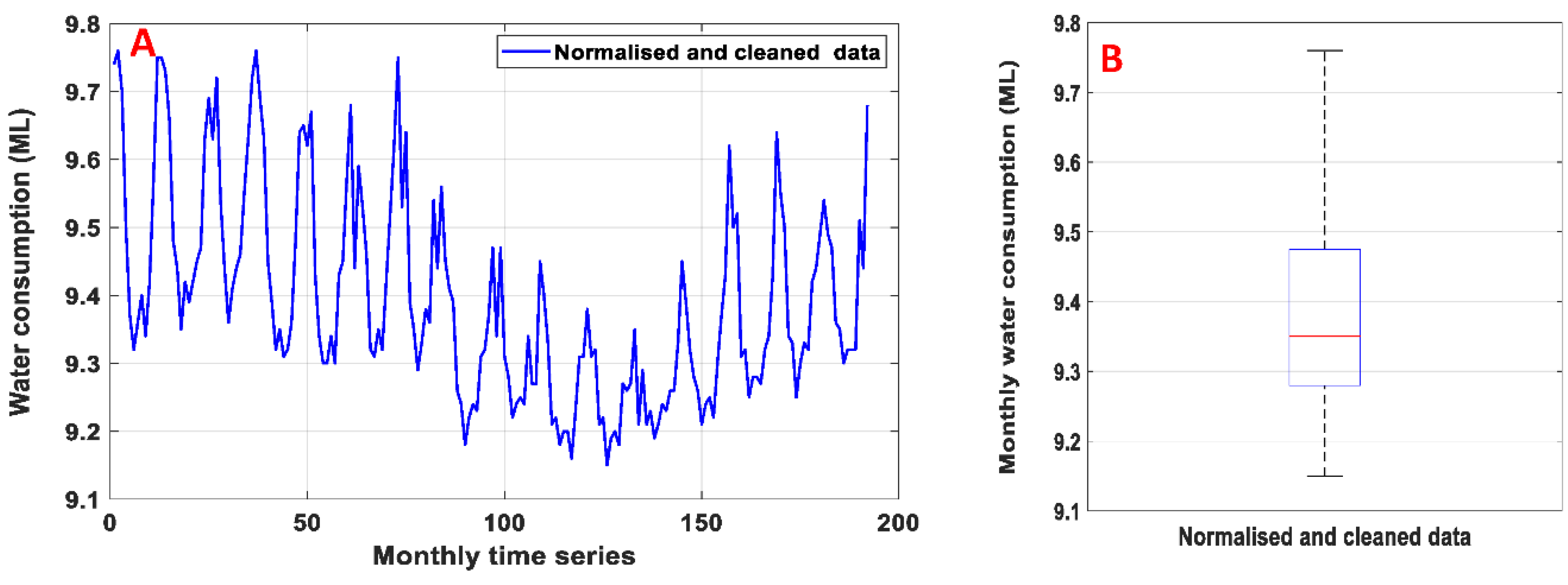
Firstly, data on water consumption and 10 climatic factors were normalised and cleaned according to Section 3.1. Figure 3 shows the normalised and cleaned water data. Figure 3A shows that the variance of the seasonal periods along the time series had been reduced in comparison to Figure 1A. Figure 3B shows that the time series, after the normalisation and treating of the outliers, tended to follow a normal distribution in comparison with Figure 1B.
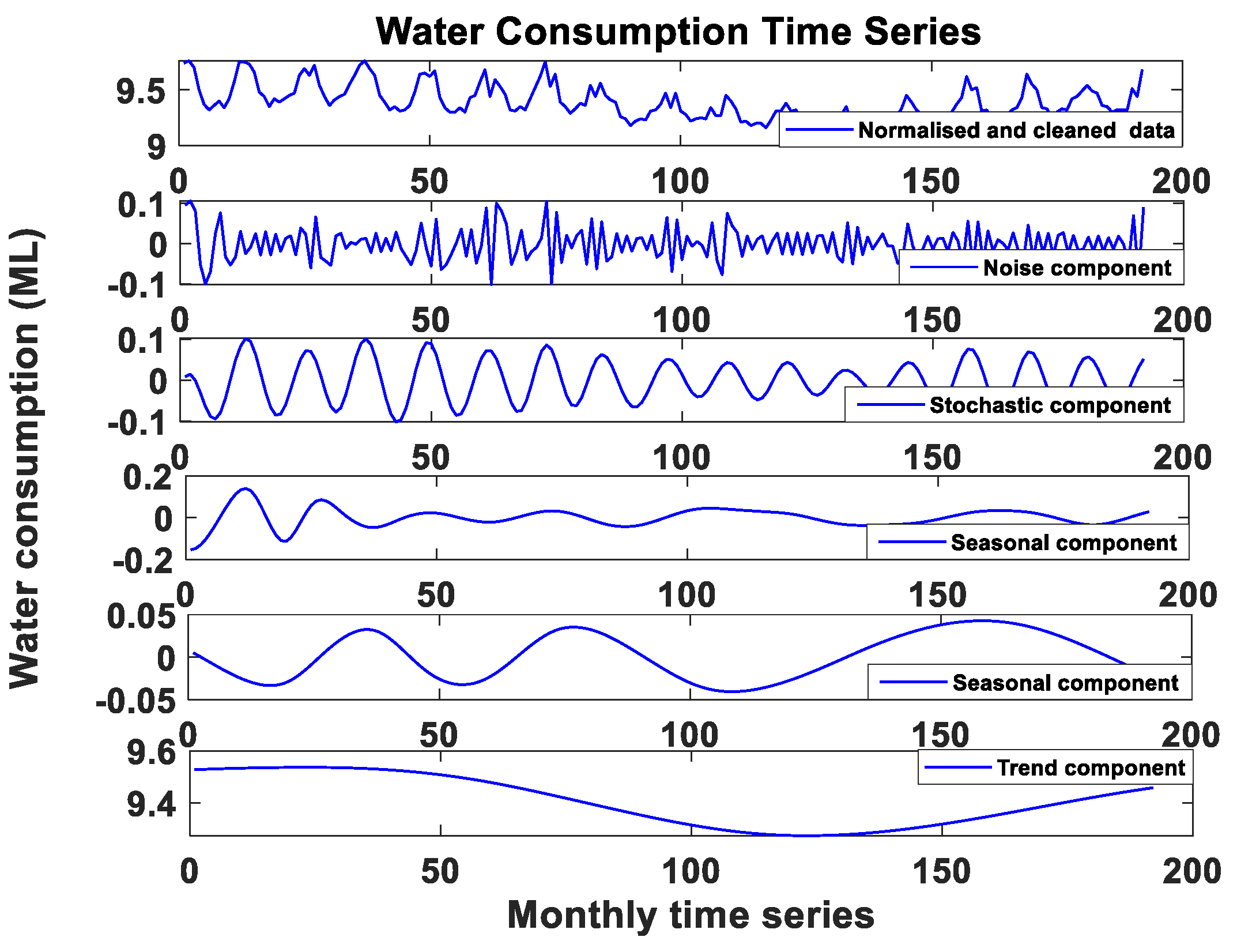
Then, the EMD approach was applied to analyse the normalised data of water consumption and all climatic factors to unravel the stochastic components of each time series. Figure 4 presents the normalised and cleaned data for water consumption and its decomposed components, including trend, seasonal, stochastic and noise. The Augmented Dickey–Fuller and Kwiatkowski–Phillips–Schmidt–Shin tests were used to assess the stationarity of the stochastic component for each factor (i.e., these two tests are used to test and select the stochastic signal). It can also be seen that other components (trend and seasonal) represented the deterministic signal, which was driven by socio-economic factors.
Table 1 presents the correlation coefficients between water consumption and climatic factors time series in the raw and stochastic stage. The table shows that data pre-processing techniques produced significant improvements in the quality of the data, such as increasing the correlation coefficient between water consumption and maximum temperature time series (from 0.63 to 0.93). Additionally, the correlation coefficient between the stochastic signal of water consumption and climatic factors over 16 years confirmed the relation between water consumption and climatic factors.
In the final stage of data pre-processing, a tolerance method was used to locate the best scenario of independent factors, climatic factors, that could accurately simulate the stochastic component of water demand and omit redundant factors to avoid multi-collinearity. The tolerance values for all of the climatic factors in the initial stage were less than the minimum limit of acceptance (i.e., it should be more than 0.1) except the Rain, which had a tolerance value equal to 0.43. So, the climatic factors that had multi-collinearity were removed separately, one by one, until the tolerance values of the selected model reached more than 0.1, as shown in Table 2. The latter shows that Tmax, RHmin and Rain were selected to be the best scenario of independent factors based on the tolerance value. As presented in Table 2, the tolerance value for each climatic factor was more than 0.1, which means the multi-collinearity assumption was not violated.
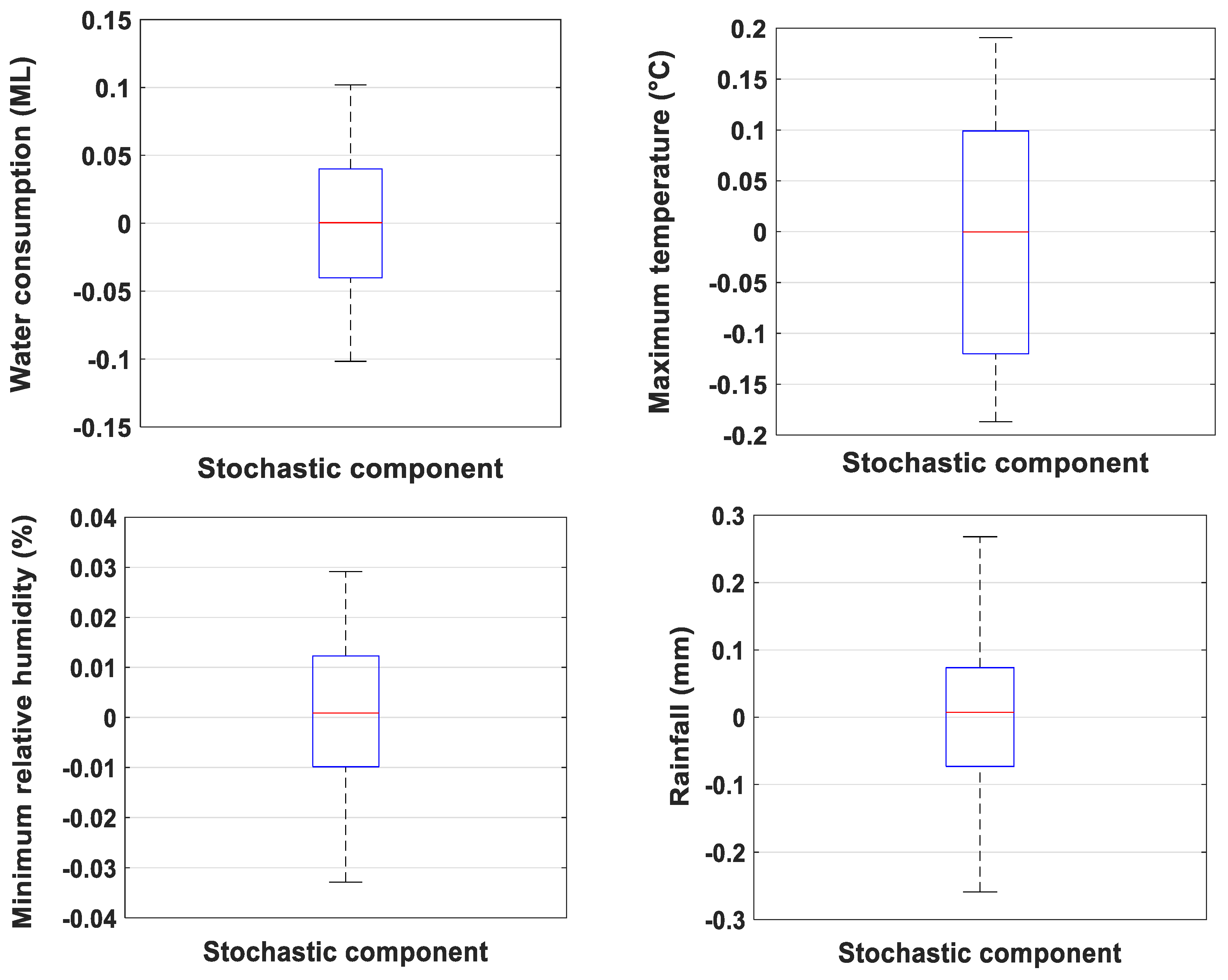
Another graphical technique can show the significance of data pre-processing. Figure 5 presents the box plot of the stochastic components of water consumption, Tmax, RHmin and Rain. It can be seen that there were no outliers within the data, and the median was zero for water consumption and Tmax, and nearly zero for all RHmin and Rain factors. The stochastic components of all factors showed a normal distribution, which was confirmed by the Kolmogorov–Smirnov test with significance values (Sig.) of more than 0.05 (i.e., the Sig. values were 2 for both minimum relative humidity and rainfall factors). Additionally, Figure 5 reveals how the EMD technique enhanced the normal distribution of water consumption compared to the distribution of water consumption in Figure 3B.
After preparing the stochastic signals of the dependent and independent factors, data were organised into three sets (as mentioned in Section 3.3): training (70%, 134 datapoints), testing (15%, 29 datapoints) and validation (15%, 29 datapoints) to build and assess the prediction model. Accordingly, this was to ensure that each dataset had data selected from along total time series (i.e., the values of the key statistical parameters, such as the maximum limit, minimum limit and standard deviation for the mentioned datasets were very comparable).

4.2. Model Configuration

The ANN model needed to be integrated with the metaheuristic algorithm to determine the optimum hyperparameters of the ANN model, including LR, N1 and N2. Thus, the SMA algorithm was hybridized with the ANN model, and the results, for more validation, were compared with the MVO-ANN and BSA-ANN algorithms. Each algorithm was run five times based on population sizes (10, 20, 30, 40 and 50 popsize) with 200 iterations to increase the solution range, as depicted in Figure 6. It can be noticed that popsize of 50 offered the best solution for all hybrid algorithms based on the fitness function (RMSE) (i.e., offered the lowest RMSE value).
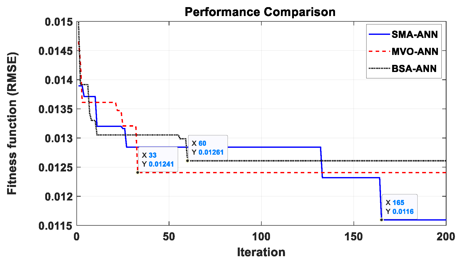
For a closer inspection of the 50 popsize of all of the three hybrid algorithms, Figure 7 shows that the SMA-ANN algorithm yielded the lowest RMSE (0.0116) after 165 iterations, while the RMSE was 0.01241 (after 33 iterations) and 0.01261 (after 60 iterations) for the MVO-ANN and BSA-ANN algorithms, respectively. That meant that the MVO-ANN and BSA-ANN algorithms did not improve their performance, based on the value of fitness function (RMSE), along with the iteration limit. For these reasons, SMA-ANN was a better choice to determine the hyperparameters of the ANN approach compared to the MVO-ANN and BSA-ANN algorithms. So, the 50 popsize of the SMA-ANN algorithm offered LR, N1 and N2 values of 0.7094, 2 and 6, respectively.
To scrutinise and validate the influence of integrating the ANN model with the SMA algorithm, the performance of the ANN technique was inspected. Thus, wide scenarios of the trial and error process were used to select the hyperparameters of the ANN technique. The outcomes presented that the values of hyperparameters were LR = 0.6, N1 = 2 and N2 = 3.

4.3. Performance Evaluation

After determining the hyperparameters of the ANN model, the ANN model became ready to simulate the monthly stochastic signal of municipal water demand. The ANN model was implemented several times to get a better network (weights) that could accurately predict the water demand. Different types of statistical tests were used to assess the ability of the model to forecast water demand based on climatic factors (validation stage).
Three statistical metrics were applied to examine the ability of the model to generalise data in the validation stage and compare the results of the SMA-ANN with the ANN model. Table 3 provides three metrics, MAE, MSE (absolute error) and MARE (relative error), to assess the non-linear dependency between the actual and simulated water demand for both models. According to Dawson et al. [56], both models showed good accuracy, but the SMA-ANN could predict water demand rather well based on the MARE value.
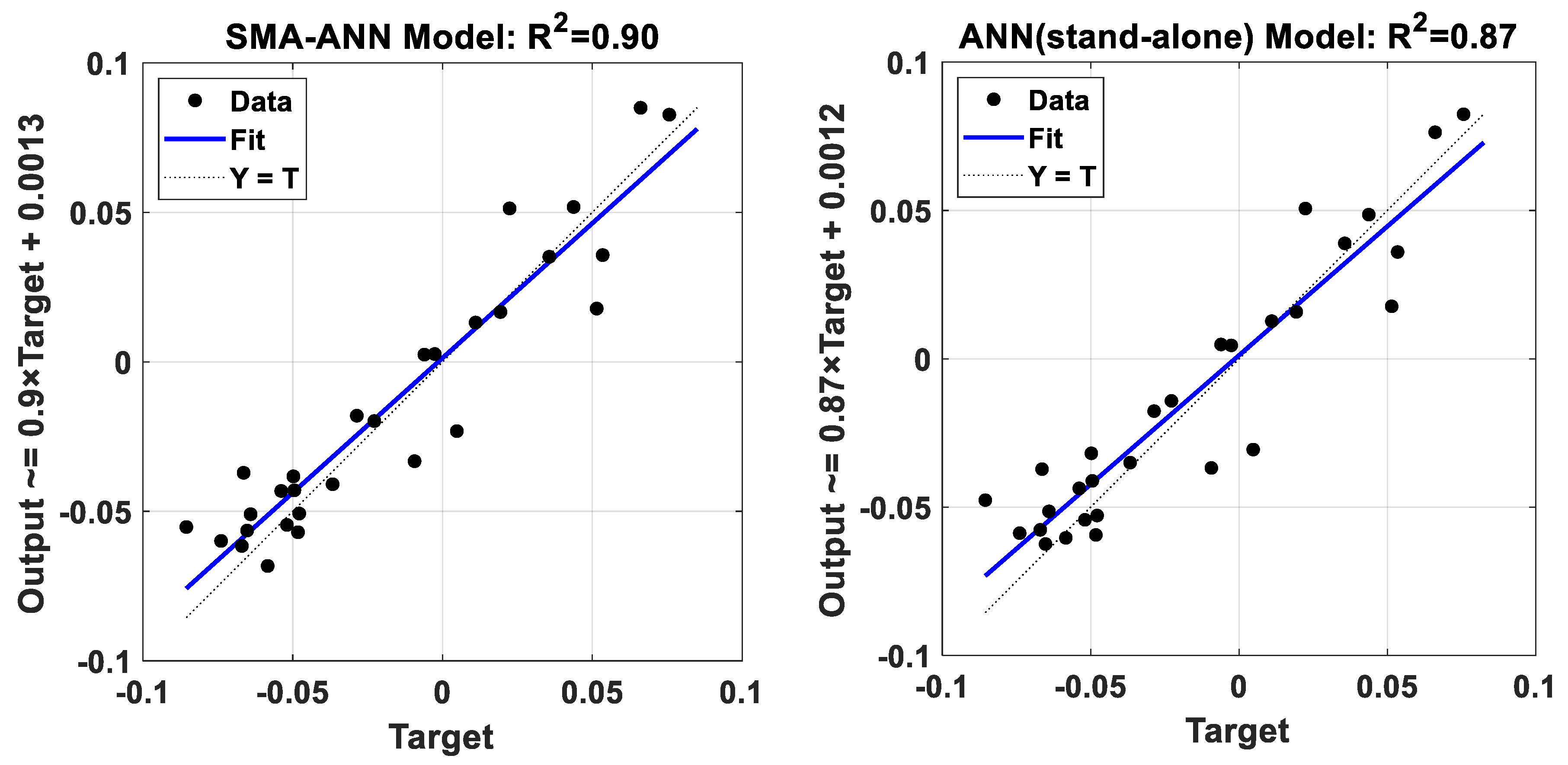
In addition, Figure 8 presents the coefficient of determination (R2) for the SMA-ANN and ANN models. The values of R2 delivered information for the linear relationship between the actual water consumption (Target, ML) and predicted water demand (Output, ML) for both models. Similar to the error tests (absolute and relative), both models offered good results according to Dawson et al. [56]. However, the value of R2 for the SMA-ANN model was 0.9, which is more accurate than that of the ANN model (0.87). Additionally, the scatter data for the SMA-ANN model were falling closer to the ideal line than the scatter data for the ANN model.
Figure 9 shows the Bland–Altman for the SMA-ANN and ANN models. The SMA-ANN has a mean = −0.002998 ML with limits of the agreement being −0.03358 and 0.02759 ML, while these values for the ANN model were −0.003439, −0.03536 and 0.02947 ML for the mean, lower and upper limits of agreement area, respectively. Additionally, a good agreement was noticed for the SMA-ANN model because up to 97% of the data were scattered between the limits of agreement, whereas the proportion was 90% for the ANN model. Generally, the obtained results revealed that the SMA-ANN model had limits of agreement much closer to the mean, and it had a higher agreement percentage compared to the ANN model. Additionally, there was no trend in the scattered data for both Figure 8 and Figure 9, and the randomness of the residual data was assessed and confirmed using the ADF test. That meant the tolerance method was successfully used to select the best model input.
The obtained results emphasised that the determination of the ANN’s parameters using hybridisation with the SMA algorithm was better than that conducted by trial and error procedure. In the former process (i.e., SMA-ANN), the parameters were determined automatically, whereas the latter was conducted manually.
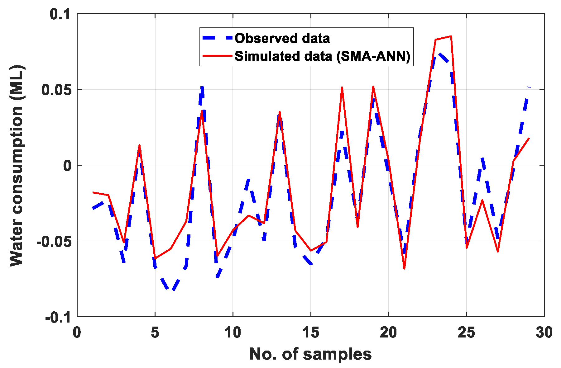
All the statistical tests examined and validated the SMA-ANN model and, for more examination, ADF and KPSST tests were used to check the stationarity of the simulated stochastic signal of water demand and residual analysis. The results showed that the simulated time series of water demand was stationary and the residual data were normally distributed, which was assessed by the Kolmogorov–Smirnov test. Furthermore, a graphical test was used to confirm the SMA-ANN model by comparing the observed and simulated water time series in the validation stage as shown in Figure 10, which shows that the model could closely follow the trend and cycles of the observed stochastic time series based on the scale of error. There were several slight deviations in the simulated time series that may have came from the influence of fluctuation of the climatic factors. However, based on both scale of error and the result of the Bland–Altman for the SMA-ANN, the error could be considered statistically insignificant.
The most interesting conclusions that could be drawn from the above results were: (1) the EMD technique had a significant rule to decompose the raw data to select the stochastic signals of dependent and independent variables. Additionally, the tolerance method was effective in determining the best scenario of independent factors. (2) The optimal hyperparameters of the ANN model were determined based on the novel hybrid model, SMA-ANN, which outperformed both MVO-ANN and BSA-ANN algorithms depending on the RMSE value. (3) The novel combined methodology that comprised data analytic and machine learning could effectively simulate the stochastic signal of water demand concerning climatic factors. (4) An automated machine learning outperformed trial and error procedure based on several statistical tests. (5) Using three metaheuristic algorithms to build the prediction model and validate the results by the ANN (stand-alone) and employing 10 climatic factors decreased the uncertainty and increased the forecasting range. (6) The hybridisation of the model, as well as the way of categorisation of the training, testing and validation samples, presented a promising application of the developed model for covering unknown extreme events, particularly when it was applied to predict data that were not used before in the model configuration. (7) The research provided important scientific insights for managers and policymakers in SEW utility to manage the water supply system under sudden increases in water demand due to the variability of the stochastic pattern of climatic factors. They could, for example, feed the model with predicting climatic factors to forecast water demand for medium-term (i.e., future). After that, they could compare the water demand in the future with the capacity of the water system and decide whether the water system is capable of successfully working under the extreme events or not. (8) The obtained results confirmed the association between climate change and water demand for the medium term.

5. Conclusions

In this study, the potential of novel coupled data pre-processing and automated machine learning for monthly stochastic urban water demand prediction based on several climatic factors was investigated. Data for water consumption and 10 climatic factors for the South East Water utility in Melbourne were utilised for building and assessing the proposed methodology. Data pre-processing techniques were considered to analyse and select the stochastic signals of water consumption and climatic factors time series by EMD approach, and to detect the best independent variables by the tolerance method. The automated machine learning included the ANN model, which integrated with the SMA algorithm to find optimal hyperparameters of the ANN model. The results highlighted the importance of data pre-processing to prepare the stochastic pattern of dependent and independent variables and to select the best scenario of independent variables. Additionally, the SMA-ANN was found to be superior to both the BSA-ANN and MVO-ANN algorithms based on RMSE as an objective function. Moreover, the performance of the hybrid model, SMA-ANN, was more accurate than the ANN (stand-alone) approach depending on different statistical tests. Furthermore, the outcomes indicated that the suggested methodology can be successfully applied in regions that suffer from climate change (i.e., drought), such as Melbourne. Consequently, the South East Water utility can take advantage of this study’s findings to establish effective strategies for optimised system operation and to maintain a balance between water requested and delivered. It also helps to establish appropriate pricing plans, schedule new changes in the network and optimise the operating procedures, such as pumps, to enhance the water quality, and to reduce the uncertainty. Based on recent literature, severe weather will probably become more common in the future. Thus, there is an urgent need for more studies that use the same or different data analytic and artificial intelligence techniques to simulate the stochastic component of urban water demand based on climate factors for regions that suffer from climate change. However, the availability of reliable data for water consumption and climatic factors for the medium or long term is considered a principal limitation of this methodology.

Author Contributions

Formal analysis, S.L.Z. and K.S.H.; data curation, S.K.G. and H.M.R.; investigation, H.A.-B.; Resources, P.K.; project administration, R.A.-K., methodology, I.H.A.; review & editing, F.F.A.-Q.; M.M., conceptualization. All authors have read and agreed to the published version of the manuscript.

Funding

This research received no external funding.

Conflicts of Interest

The authors declare no conflict of interest.

References

  1. Farhan, S.L.; Abdelmonem, M.G.; Nasar, Z.A. The Urban Transformation of Traditional City Centres: Holy Karbala as a Case Study. Int. J. Archit. Res. ArchNet-IJAR 2018, 12, 53–67. [Google Scholar] [CrossRef]
  2. Farhan, S.L.; Jasim, I.A.; Al-Mamoori, S.K. The transformation of the city of Najaf, Iraq: Analysis, reality and future prospects. J. Urban. Regen. Renew. 2019, 13, 160–171. [Google Scholar]
  3. Zubaidi, S.L.; Kot, P.; Hashim, K.; Alkhaddar, R.; Abdellatif, M.; Muhsin, Y.R. Using LARS–WG model for prediction of temperature in Columbia City, USA. IOP Conf. Ser. Mater. Sci. Eng. 2019, 584, 1–9. [Google Scholar] [CrossRef]
  4. Hashim, K.S.; Kot, P.; Zubaidi, S.L.; Alwash, R.; Al Khaddar, R.; Shaw, A.; Al-Jumeily, D.; Aljefery, M.H. Energy Efficient Electrocoagulation Using Baffle-Plates Electrodes for Efficient Escherichia Coli Removal from Wastewater. J. Water Process. Eng. 2020, 33, 1–7. [Google Scholar] [CrossRef]
  5. Rahim, M.S.; Nguyen, K.A.; Stewart, R.A.; Giurco, D.; Blumenstein, M. Machine Learning and Data Analytic Techniques in Digital Water Metering: A Review. Water 2020, 12, 294. [Google Scholar] [CrossRef] [Green Version]
  6. Hemati, A.; Rippy, M.A.; Grant, S.B.; Davis, K.; Feldman, D. Deconstructing Demand: The Anthropogenic and Climatic Drivers of Urban Water Consumption. Environ. Sci. Technol. 2016, 50, 12557–12566. [Google Scholar] [CrossRef]
  7. Roy, U.; Majumder, M. Vulnerability of Watersheds to Climate Change Assessed by Neural Network and Analytical Hierarchy Process; Springer: New York, NY, USA, 2016; Volume 3, p. 97. [Google Scholar] [CrossRef]
  8. Zubaidi, S.L.; Ortega-Martorell, S.; Kot, P.; Alkhaddar, R.M.; Abdellatif, M.; Gharghan, S.K.; Ahmed, M.S.; Hashim, K. A Method for Predicting Long-Term Municipal Water Demands Under Climate Change. Water Resour. Manag. 2020, 34, 1265–1279. [Google Scholar] [CrossRef]
  9. Altunkaynak, A.; Nigussie, T.A. Monthly water demand prediction using wavelet transform, first-order differencing and linear detrending techniques based on multilayer perceptron models. Urban Water J. 2018, 15, 177–181. [Google Scholar] [CrossRef]
  10. Rasifaghihi, N.; Li, S.S.; Haghighat, F. Forecast of urban water consumption under the impact of climate change. Sustain. Cities Soc. 2020, 52. [Google Scholar] [CrossRef]
  11. Ebrahim Banihabib, M.; Mousavi-Mirkalaei, P. Extended linear and non-linear auto-regressive models for forecasting the urban water consumption of a fast-growing city in an arid region. Sustain. Cities Soc. 2019, 48. [Google Scholar] [CrossRef]
  12. Pacchin, E.; Alvisi, S.; Franchini, M. A Short-Term Water Demand Forecasting Model Using a Moving Window on Previously Observed Data. Water 2017, 9, 172. [Google Scholar] [CrossRef]
  13. House-Peters, L.A.; Chang, H. Urban water demand modeling: Review of concepts, methods, and organizing principles. Water Resour. Res. 2011, 47. [Google Scholar] [CrossRef] [Green Version]
  14. Donkor, E.A.; Mazzuchi, T.H.; Soyer, R.; Roberson, J.A. Urban water demand forecasting: Review of methods and models. J. Water Resour. Planing Manag. 2014, 140, 146–159. [Google Scholar] [CrossRef]
  15. Ghalehkhondabi, I.; Ardjmand, E.; Young, W.A., II; Weckman, G.R. Water demand forecasting: Review of soft computing methods. Environ. Monit. Assess. 2017, 189, 313. [Google Scholar] [CrossRef]
  16. De Souza Groppo, G.; Costa, M.A.; Libânio, M. Predicting water demand: A review of the methods employed and future possibilities. Water Supply 2019. [Google Scholar] [CrossRef]
  17. Candelieri, A. Clustering and Support Vector Regression for Water Demand Forecasting and Anomaly Detection. Water 2017, 9, 224. [Google Scholar] [CrossRef]
  18. Firat, M.; Turan, M.E.; Yurdusev, M.A. Comparative analysis of fuzzy inference systems for water consumption time series prediction. J. Hydrol. 2009, 374, 235–241. [Google Scholar] [CrossRef]
  19. Chen, G.; Long, T.; Xiong, J.; Bai, Y. Multiple Random Forests Modelling for Urban Water Consumption Forecasting. Water Resour. Manag. 2017, 31, 4715–4729. [Google Scholar] [CrossRef]
  20. Altunkaynak, A.; Nigussie, T.A. Monthly Water Consumption Prediction Using Season Algorithm and Wavelet Transform–Based Models. J. Water Resour. Plan. Manag. 2017, 143. [Google Scholar] [CrossRef]
  21. Mouatadid, S.; Adamowski, J. Using extreme learning machines for short-term urban water demand forecasting. Urban. Water J. 2016, 14, 630–638. [Google Scholar] [CrossRef]
  22. Zubaidi, S.L.; Dooley, J.; Alkhaddar, R.M.; Abdellatif, M.; Al-Bugharbee, H.; Ortega-Martorell, S. A Novel approach for predicting monthly water demand by combining singular spectrum analysis with neural networks. J. Hydrol. 2018, 561, 136–145. [Google Scholar] [CrossRef]
  23. Mirjalili, S.; Mirjalili, S.M.; Hatamlou, A. Multi-Verse Optimizer: A nature-inspired algorithm for global optimization. Neural Comput. Appl. 2015, 27, 495–513. [Google Scholar] [CrossRef]
  24. Ullah, I.; Hussain, I.; Uthansakul, P.; Riaz, M.; Khan, M.N.; Lloret, J. Exploiting Multi-Verse Optimization and Sine-Cosine Algorithms for Energy Management in Smart Cities. Appl. Sci. 2020, 10, 2095. [Google Scholar] [CrossRef] [Green Version]
  25. Wang, X.; Pan, J.-S.; Chu, S.-C. A Parallel Multi-Verse Optimizer for Application in Multilevel Image Segmentation. IEEE Access 2020, 8, 32018–32030. [Google Scholar] [CrossRef]
  26. Zubaidi, S.L.; Ortega-Martorell, S.; Al-Bugharbee, H.; Olier, I.; Hashim, K.S.; Gharghan, S.K.; Kot, P.; Alkhaddar, R.M. Urban Water Demand Prediction for a City That Suffers from Climate Change and Population Growth: Gauteng Province Case Study. Water 2020, 12, 1885. [Google Scholar] [CrossRef]
  27. Zhang, Y.; Jin, Z.; Zhao, X.; Yang, Q.J. Backtracking search algorithm with Lévy flight for estimating parameters of photovoltaic models. Energy Convers. Manag. 2020, 208, 112615. [Google Scholar] [CrossRef]
  28. Mehmood, A.; Shi, P.; Raja, M.A.Z.; Zameer, A.; Chaudhary, N.I. Design of backtracking search heuristics for parameter estimation of power signals. Neural Comput. Appl. 2020. [Google Scholar] [CrossRef]
  29. Li, S.; Chen, H.; Wang, M.; Heidari, A.A.; Mirjalili, S. Slime mould algorithm: A new method for stochastic optimization. Futur. Gener. Comput. Syst. 2020, 111, 300–323. [Google Scholar] [CrossRef]
  30. Ghafil, H.N.; Jármai, K. Dynamic differential annealed optimization: New metaheuristic optimization algorithm for engineering applications. Appl. Soft Comput. 2020, 93, 106392. [Google Scholar] [CrossRef]
  31. Jiao, S.; Chong, G.; Huang, C.; Hu, H.; Wang, M.; Heidari, A.A.; Chen, H.; Zhao, X. Orthogonally adapted Harris Hawk Optimization for parameter estimation of photovoltaic models. Energy 2020, 203, 117804. [Google Scholar] [CrossRef]
  32. Rodríguez-Esparza, E.; Zanella-Calzada, L.A.; Oliva, D.; Heidari, A.A.; Zaldivar, D.; Pérez-Cisneros, M.; Foong, L.K. An Efficient Harris Hawks-inspired Image Segmentation Method. Exert Syst. Appl. 2020, 155, 113428. [Google Scholar] [CrossRef]
  33. Zubaidi, S.L.; Kot, P.; Alkhaddar, R.M.; Abdellatif, M.; Al-Bugharbee, H. Short-Term Water Demand Prediction in Residential Complexes: Case Study in Columbia City, USA. In Proceedings of the 2018 11th International Conference on Developments in eSystems Engineering (DeSE), Cambridge, UK, 2–5 September 2018; pp. 31–35. [Google Scholar]
  34. Zubaidi, S.L.; Al-Bugharbee, H.; Muhsen, Y.R.; Hashim, K.; Alkhaddar, R.M.; Hmeesh, W.H. The Prediction of Municipal Water Demand in Iraq: A Case Study of Baghdad Governorate. In Proceedings of the 2019 12th International Conference on Developments in eSystems Engineering (DeSE), Kazan, Russia, 7–10 October 2019; pp. 274–277. [Google Scholar]
  35. Campisi-Pinto, S.; Adamowski, J.; Oron, G. Forecasting Urban Water Demand Via Wavelet-Denoising and Neural Network Models. Case Study: City of Syracuse, Italy. Water Resour. Manag. 2012, 26, 3539–3558. [Google Scholar] [CrossRef]
  36. Seo, Y.; Kwon, S.; Choi, Y. Short-Term Water Demand Forecasting Model Combining Variational Mode Decomposition and Extreme Learning Machine. Hydrology 2018, 5, 54. [Google Scholar] [CrossRef] [Green Version]
  37. Vecchio, A.; Anzidei, M.; Serpelloni, E.; Florindo, F. Natural Variability and Vertical Land Motion Contributions in the Mediterranean Sea-Level Records over the Last Two Centuries and Projections for 2100. Water 2019, 11, 1480. [Google Scholar] [CrossRef] [Green Version]
  38. Chu, T.-Y.; Huang, W.-C. Application of Empirical Mode Decomposition Method to Synthesize Flow Data: A Case Study of Hushan Reservoir in Taiwan. Water 2020, 12, 927. [Google Scholar] [CrossRef] [Green Version]
  39. Gedefaw, M.; Hao, W.; Denghua, Y.; Girma, A.; Khamis, M.I. Variable selection methods for water demand forecasting in Ethiopia: Case study Gondar town. Cogent Environ. Sci. 2018, 4. [Google Scholar] [CrossRef]
  40. Haque, M.M.; Rahman, A.; Hagare, D.; Chowdhury, R.K. A Comparative Assessment of Variable Selection Methods in Urban Water Demand Forecasting. Water 2018, 10, 419. [Google Scholar] [CrossRef] [Green Version]
  41. Zhang, X.; Qiu, J.; Leng, G.; Yang, Y.; Gao, Q.; Fan, Y.; Luo, J. The Potential Utility of Satellite Soil Moisture Retrievals for Detecting Irrigation Patterns in China. Water 2018, 10, 1505. [Google Scholar] [CrossRef] [Green Version]
  42. Kim, K.; Joo, H.; Han, D.; Kim, S.; Lee, T.; Kim, H.S. On Complex Network Construction of Rain Gauge Stations Considering Nonlinearity of Observed Daily Rainfall Data. Water 2019, 11, 1578. [Google Scholar] [CrossRef] [Green Version]
  43. Zubaidi, S.L.; Gharghan, S.K.; Dooley, J.; Alkhaddar, R.M.; Abdellatif, M. Short-Term Urban Water Demand Prediction Considering Weather Factors. Water Resour. Manag. 2018, 32, 4527–4542. [Google Scholar] [CrossRef]
  44. MW. Corporate Plan 2016/17 to 2020/21; MW: Victoria, Australia, 2017; p. 39. [Google Scholar]
  45. SEW. South East Water Annual Report 2015-16; Including the Financial Report; SEW: Queensland, Australia, 2016. [Google Scholar]
  46. Araghinejad, S. Data-Driven Modeling: Using MATLAB® in Water Resources and Environmental Engineering; Springer: New York, NY, USA, 2014. [Google Scholar] [CrossRef]
  47. Tabachnick, B.G.; Fidell, L.S. Using Multivariate Statistics, Sixth ed.; Pearson Education, Inc.: New York, NY, USA, 2013. [Google Scholar]
  48. Bailey, O.; Zlatanovic, L.; van der Hoek, J.P.; Kapelan, Z.; Blokker, M.; Arnot, T.; Hofman, J. A Stochastic Model to Predict Flow, Nutrient and Temperature Changes in a Sewer under Water Conservation Scenarios. Water 2020, 12, 1187. [Google Scholar] [CrossRef] [Green Version]
  49. Tabrizi, A.A.; Al-Bugharbee, H.; Trendafilova, I.; Garibaldi, L. A cointegration-based monitoring method for rolling bearings working in time-varying operational conditions. Meccanica 2017, 52, 1201–1217. [Google Scholar] [CrossRef] [Green Version]
  50. Abdou, A.D.; Ngom, N.F.; Sidibé, S.; Niang, O.; Thioune, A.; Ndiaye, C.H. Neural networks for biomedical signals classification based on empirical mode decomposition and principal component analysis. In Innovation and Interdisciplinary Solutions for Underserved Areas; Springer: New York, NY, USA, 2017; pp. 267–278. [Google Scholar]
  51. Zeiler, A.; Faltermeier, R.; Keck, I.R.; Tomé, A.M.; Puntonet, C.G.; Lang, E.W. Empirical mode decomposition-an introduction. In Proceedings of the 2010 International Joint Conference on Neural Networks (IJCNN), Barcelona, Spain, 18–23 July 2010; pp. 1–8. [Google Scholar]
  52. Pallant, J. SPSS Survival Manual: A Step by Step Guide to Data Analysis Using IBM SPSS; Open University Press/McGraw-Hill: London, UK, 2016. [Google Scholar]
  53. Bayatvarkeshi, M.; Mohammadi, K.; Kisi, O.; Fasihi, R. A new wavelet conjunction approach for estimation of relative humidity: Wavelet principal component analysis combined with ANN. Neural Comput. Appl. 2018. [Google Scholar] [CrossRef]
  54. Zubaidi, S.L.; Al-Bugharbee, H.; Ortega-Martorell, S.; Gharghan, S.K.; Olier, I.; Hashim, K.S.; Al-Bdairi, N.S.S.; Kot, P. A Novel Methodology for Prediction Urban Water Demand by Wavelet Denoising and Adaptive Neuro-Fuzzy Inference System Approach. Water 2020, 12, 1628. [Google Scholar] [CrossRef]
  55. González Perea, R.; Camacho Poyato, E.; Montesinos, P.; Rodríguez Díaz, J.A. Optimisation of water demand forecasting by artificial intelligence with short data sets. Biosyst. Eng. 2019, 177, 59–66. [Google Scholar] [CrossRef]
  56. Dawson, C.W.; Abrahart, R.J.; See, L.M. HydroTest: A web-based toolbox of evaluation metrics for the standardised assessment of hydrological forecasts. Environ. Model. Softw. 2007, 22, 1034–1052. [Google Scholar] [CrossRef] [Green Version]
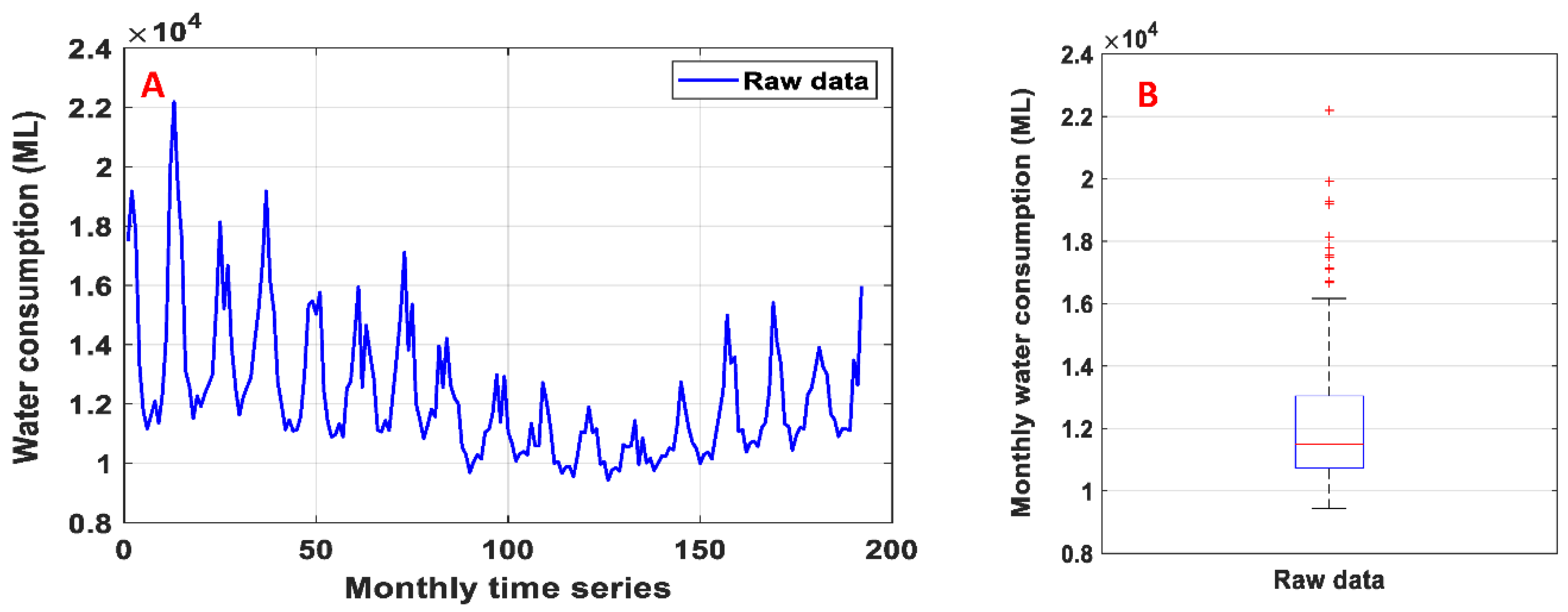
Figure 1. (A) Monthly time series, (B) box plot of municipal water consumption for SEW utility.
Water 12 02692 g001
Figure 2. The proposed methodology for predicting water demand based on climatic factors.
Water 12 02692 g002
Figure 3. (A) Monthly time series, (B) box plot of normalised and cleaned municipal water consumption data.
Water 12 02692 g003
Figure 4. Normalised and cleaned water time series and the first five components obtained by EMD.
Water 12 02692 g004
Figure 5. Box plot of monthly stochastic components for water consumption and climatic factors.
Water 12 02692 g005
Figure 6. Performance of SMA-ANN, MVO-ANN and BSA-ANN algorithms.
Water 12 02692 g006
Figure 7. Performance comparison of the best popsize of SMA-ANN, MVO-ANN and BSA-ANN algorithms.
Water 12 02692 g007
Figure 8. The performance of SMA-ANN and ANN techniques in the validation stage.
Water 12 02692 g008
Figure 9. Bland–Altman plot of SMA-ANN and ANN techniques in the validation stage.
Water 12 02692 g009
Figure 10. A comparison between observed and simulated stochastic data in the validation stage.
Water 12 02692 g010
Table 1. Correlation coefficients between water consumption and climatic factors in the raw and stochastic stage.
DataTmaxTminTmeanRainEvaSradVPRHmaxRHminFA-O56
Raw0.630.610.62−0.100.610.600.55−0.59−0.540.63
Stochastic0.930.910.92−0.530.880.830.88−0.89−0.750.88
Table 2. Collinearity statistics to the selected model input.
Climatic FactorsTolerance Value
Tmax0.322
RHmin0.344
Rain0.867
Table 3. Statistical indicators of SMA-ANN and ANN models in the validation stage.
ModelsMAERMSEMARE
SMA-ANN0.0120.0150.001
ANN0.0130.0170.015