Article

Spatiotemporal Variation in Phytoplankton Community Driven by Environmental Factors in the Northern East China Sea

1
Department of Oceanography, Pusan National University, Busan 46241, Korea
2
Oceanic Climate & Ecology Research Division, National Institute of Fisheries Science, Busan 46083, Korea
*
Author to whom correspondence should be addressed.
Water 2020, 12(10), 2695; https://doi.org/10.3390/w12102695
Submission received: 13 July 2020 / Revised: 10 September 2020 / Accepted: 24 September 2020 / Published: 26 September 2020
(This article belongs to the Special Issue Marine Nitrogen Fixation and Phytoplankton Ecology)

Abstract

:
The East China Sea (ECS) is the largest marginal sea in the northern western Pacific Ocean. In comparison to various physical studies, little information on the seasonal patterns in community structure of phytoplankton is currently available. Based on high performance liquid chromatography (HPLC) pigment analysis, spatiotemporal variations in phytoplankton community compositions were investigated in the northern ECS. Water temperature and salinity generally decreased toward the western part of the study area but warmer conditions in August led to strong vertical stratification of the water column. In general, major inorganic nutrient concentrations were considerably higher in the western part with a shallow water depth, and consistent with previous results, had no discernable vertical pattern during our observation period except in August. This study also revealed PO4-limited environmental conditions in May and August. The monthly averaged integral chlorophyll-a concentration varied seasonally, highest (35.2 ± 20.22 mg m−2) in May and lowest (5.2 ± 2.54 mg m−2) in February. No distinct vertical differences in phytoplankton community compositions were observed for all the sampling seasons except in August when cyanobacteria predominated in the nutrient-deficient surface layer and diatoms prevailed at deep layer. Canonical correlation analysis results revealed that nutrient distribution and the water temperature were the major drivers of the vertical distribution of phytoplankton communities in August. Spatially, a noticeable difference in phytoplankton community structure between the eastern and western parts was observed in November with diatom domination in the western part and cyanobacteria domination in the eastern part, which were significantly (p < 0.01) correlated with water temperature, salinity, light conditions, and nutrient concentrations. Overall, the two major phytoplankton groups were diatoms (32.0%) and cyanobacteria (20.6%) in the northern ECS and the two groups were negatively correlated, which holds a significant ecological meaning under expected warming ocean conditions.

1. Introduction

Phytoplankton communities play an important role in marine ecosystems, affecting carbon and nutrient cycling, the structure and efficiency of the food web, and the flux of particles to deep waters [1,2,3]. Phytoplankton show a clear variation in community structure and abundance in response to environmental changes, so the phytoplankton community structure can be used as a useful indicator of ecosystem and water quality characteristics [4,5,6]. Therefore, in order to understand the structure and function of the ecosystem, it is necessary to monitor the spatiotemporal changes in the phytoplankton community [7]. Various methods such as microscopy, flow cytometry, and pigment analysis have been used to quantitatively analyze phytoplankton community structure. Traditionally, microscopic methods have been the most commonly used to assess biomass and community structure [8]. Microscopes can provide detailed information on species and size, but this method requires taxonomic expertise and very considerable time. Furthermore, microscopic methods fall short when identifying small organisms such as some of picophytoplankton and nano flagellates [9], and the structure of fragile cells of many species can be altered during the process of fixation in Lugol’s solution, formaldehyde, glutar-aldehyde, and similar fixatives [10,11]. Flow-cytometric analysis has been developed for providing more rapid and automated method for identification of communities of smaller phytoplankton. Flow-cytometric analysis requires a full understanding of the optical characteristics of the species and can mainly separate phytoplankton communities into picoplanktonic prokaryotes, picoeukaryotes, and nanoeukaryotes [12,13,14]. High performance liquid chromatography (HPLC) was used for this study because HPLC method can be used to measure the concentration of each pigment separately, and possible to determine the clustering of phytoplankton using the extracted marker pigments [15]. In particular, this method can provide useful information on nano- and pico-sized phytoplankton communities that are difficult to distinguish based on microscopic observations [16].
The East China Sea (ECS) is the largest marginal sea in the northern west Pacific and approximately 70% of the area is made up of a wide continental shelf. ECS is one of the most productive areas and possible sinks of carbon dioxide [17]. Furthermore, it is considered one of the most important marine fishing grounds in China [18]. Various water masses affect in the ECS, such as the Yellow Sea bottom cold water (YSCW) from the north, Changiiang diluted water (CDW) from the world’s largest Yangtze river from the west, Kuroshio water (KW) from the east and Taiwan current warm water (TCWW) from the south [19,20,21,22]. Generally, the environmental conditions vary from the eastern part to the western part in the ECS. This complex topography and various water masses cause show heterogeneous and complex environmental characteristics seasonally and spatially [23]. Previous studies for phytoplankton community in the northern ECS are quite limited and most of the studies have focused on the Yangtze River estuary and adjacent waters [24,25,26]. Three different phytoplankton communities in the Yangtze River estuary have been identified according to water mass [27,28,29]. Diatoms are generally the most dominant groups in this area [27,28,29,30,31]. In the northern ECS near Korea, several previous studies focused on the phytoplankton community were carried out in spring [32] and summer [33,34] and mostly conducted over one season. In addition, most of the studies have focused on the spatial distribution of diatoms and dinoflagellates which can be identified under the microscope. To date, little information on the seasonal patterns in community structure that is inclusive of all phytoplankton is currently available in the northern ECS. Therefore, the present study aimed to investigate spatiotemporal changes in composition and distribution of phytoplankton community structure in the northern ECS that is possible using pigment analysis through HPLC.

2. Materials and Methods

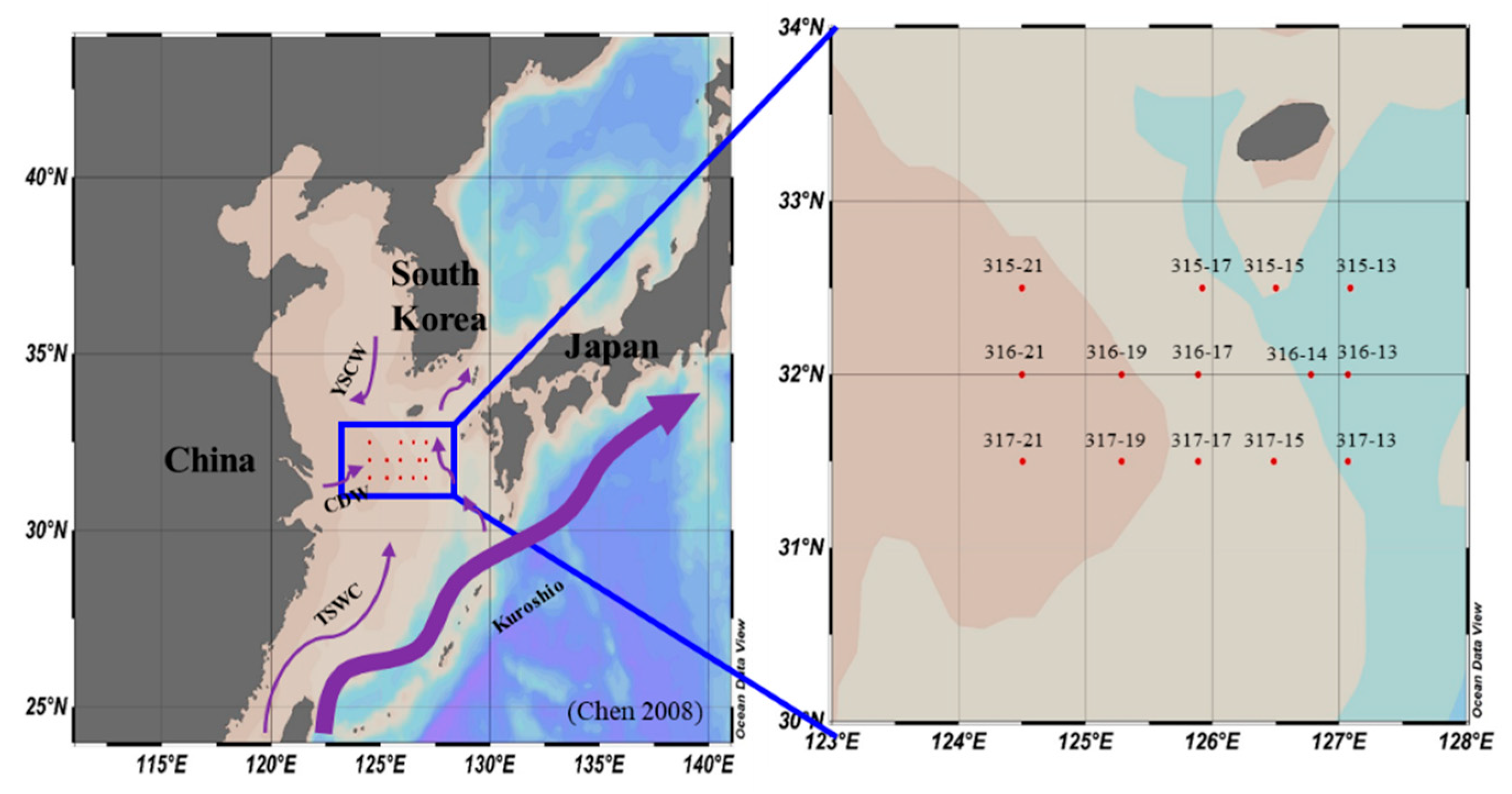
2.1. Sampling Site and Water Sampling

Four cruises were carried out in the northern ECS from 1–9 February, 30 April–10 May, 2–10 August, and 7–17 November in 2018, as representatives for winter, spring, summer, and autumn, respectively (Figure 1; Table 1). Water samples were collected from three light depths (100%, 30%, and 1% penetration of surface irradiance, PAR) using a CTD/rosette sampler fitted with Niskin bottles. The light depths were determined by a Secchi disk. Phytoplankton pigments and physicochemical parameters (temperature, salinity, and major nutrients; N, P, and Si) were analyzed in samples drawn from the three light depths. The vertical temperature and salinity were measured by SBE9/11 CTD (Sea-Bird Electronics, Bellevue, WA, USA) sensors.

2.2. Phytoplankton Pigment Analysis

Water samples for photosynthetic pigment analysis were filtered through 47 mm GF/F filters (Whatman, Maidstone, UK; 07 μm), and then stored in a freezer at −80 °C to avoid degradation. Pigments were extracted in 100% acetone (5 mL) with cantaxanthin (100 μL) as an internal standard for 24 h in the dark at 4 °C and placed in an ultra-sonic bath to disrupt a cell [35,36]. An aliquot water of 1 mL was passed through a 0.45 μm PTFE syringe filter to rid the samples of particles. After the extracts were centrifuged for 10 min at 3500 rpm to remove cellular debris and glass fibers. All procedures were carried out under low light conditions to minimize pigment degradation. Pigments were analyzed using a HPLC (Agilent Infinite 1260, Santa Clara, CA, USA), and the separation of pigments was performed using a slightly modified method of [37] and [38]. The peaks were identified based on their retention time compared with those of pure standards (chlorophyll a, chlorophyll b, β-carotene, fucoxanthin, prasinoxanthin, 19′-hexanoyloxyfucoxanthin, diadinoxanthin, 19′-butanoyloxy-fucoxanthin, peridinin, alloxanthin, neoxanthin, violaxanthin, prasinoxanthin, lutein, and zeaxanthin obtained from DHI, Denmark). The concentrations of pigments in samples were calculated as following equation. Standard response factor (Rf) was calculated based on the standard pigment and dividing the concentration of the standard by the measured peak area [38].
Concentration = Area × Rf × (Ve/Vs) [ngL−1]
  • Area = area of the peak in the sample [area]
  • Rf = standard response factor [ngL−1 area−1]
  • Ve = AIS/(peak area of IS added to sample) × (Volume of IS added to sample) [L]
  • Vs = volume of filtered water sample [L]
  • AIS = peak area of IS when 1 mL IS is mixed with 300 μL of H2O
  • IS = Internal Standard
The CHEMTAX program was used to estimate the contribution of the different phytoplankton community structure to the total chlorophyll a [15,16]. The contribution of diatoms, dinoflagellates, prymnesiophytes, chlorophytes, chrysophytes, cryptophytes, cyanobacteria and prasinophytes were calculated based on the program. Twelve pigments and initial pigment ratios for around the Korean peninsula were used for this study [38]. In the following CHEMTAX, to derive the most accurate phytoplankton groups, data was binned according to sampling month and three light depths (100%, 30% and 1% penetration of surface irradiance, PAR) [39,40].

2.3. Dissolved Inorganic Nutrient Concentration

An aliquot of water (100 mL) was filtered onboard through GF/F filters (Whatman, Maidstone, UK; 07 μm) for dissolved inorganic nutrient concentrations (NH4, NO2, NO3, PO4, and SiO2) and kept frozen (−20 °C) until further analysis. Concentrations of nutrients were determined in an automatic analyzer (Quaatro, Bran + Luebbe, Germany) belonging to the National Institute of Fisheries Science (NIFS), Korea. Dissolved inorganic nitrogen (DIN) concentrations were calculated as the sum of NH4, NO2 and NO3.
For verifying P-limited water conditions, Excess Nitrate (ExN), which is calculated as ExN = DIN-(R*PO4) (R = Redfield N:P ratio of 16), was used in this study [41,42,43]. ExN values of <0 indicate PO4-enriched condition, while ExN > 0 indicates the converse condition [41,42,43].

2.4. Statistical Analysis

Canonical correspondence analysis (CCA) was performed using “past 3” software to explain the relationship between environmental parameters and phytoplankton community structure [44]. Temperature, salinity, depth, DIN, PO4, SiO2, and ExN were include for the environmental parameters.

3. Results

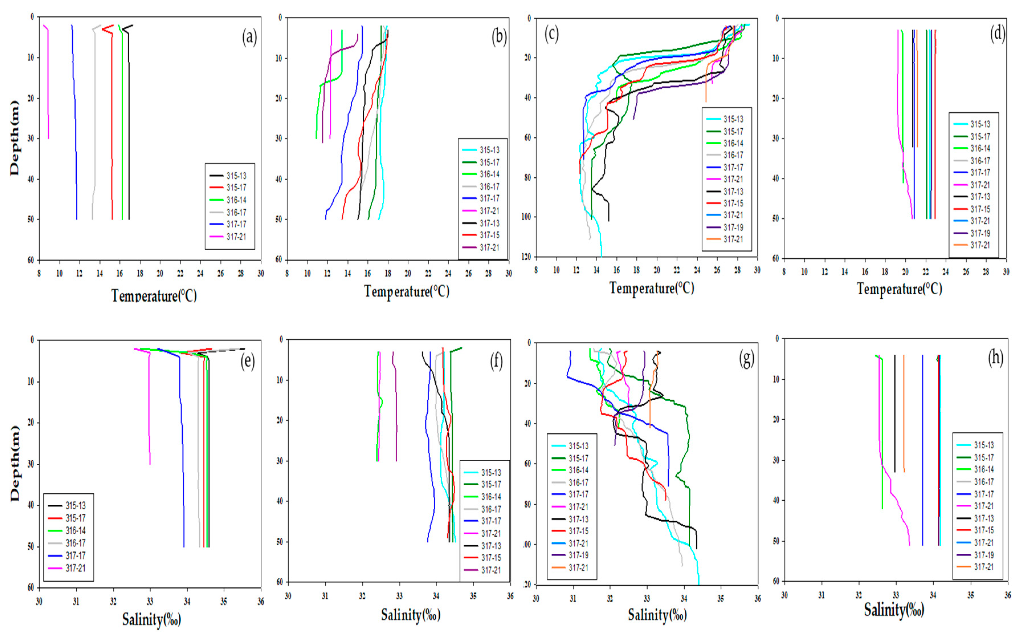
3.1. Physical Environments

Seasonal distribution patterns of temperature and salinity during the four cruises are summarized in Table 1. The average temperature was lowest in February (winter) at 13.7 ± 2.9 °C and gradually increased to highest in August (summer) at 24.2 ± 4.7 °C. The average salinity was highest at 34.1 ± 0.6 in February and lowest at 32.3 ± 0.7 in August. In February, the water temperature decreased toward the western part from the eastern part in the study area and the salinity showed the same trend as the water temperature (Table 1). The water temperature and salinity in May (spring) were also relatively higher in the eastern part and lower in the western but the difference in water temperature was smaller in May compared to that in February. On the other hand, the water temperature and salinity were inversely spatially distributed in August with low in the eastern and high in the western parts and the differences were smallest during the observation period. Vertically, the temperature increased with depth in August, which resulted in a strong stratification (Figure 2). In November (autumn), the patterns in water temperature and salinity were similar to those in February and May.

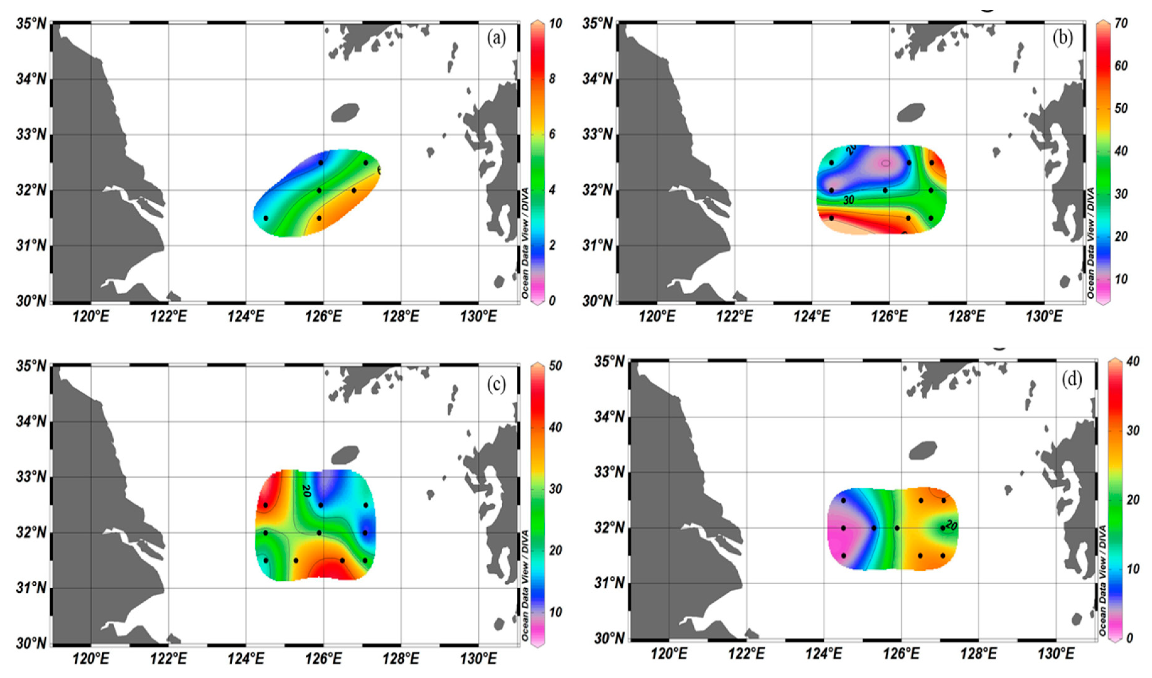
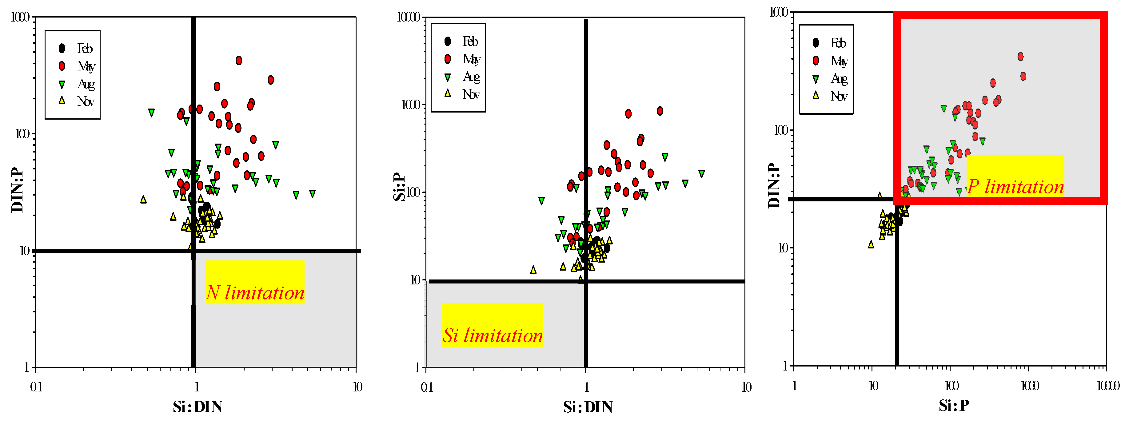
3.2. Dissolved Inorganic Nutrient Concentrations

Inorganic nutrient concentrations at the three light depths for each cruise are summarized in Table 2. DIN and PO4 concentrations were highest in February and remained low in other seasons, whereas SiO2 tended to increase from May to August and November. In February, the ranges of DIN, PO4 and SiO2 concentrations from surface to 1% light depths were 5.3–14.1 μM, 0.3–0.6 μM, and 6.0–16.8 μM, respectively. There were no distinct vertical patterns, but in the horizontal direction, DIN, PO4, and SiO2 tended to increase from the northeast to the southwest stations. In May, the ranges of DIN, PO4, and SiO2 concentrations were 2.5–12.3 μM, <0.1–0.3 μM, and 3.4–12.4 μM, respectively. No marked vertical patterns in the concentrations were observed but horizontally, DIN and SiO2 showed relatively higher in the western part compared to the eastern part in May. Generally, PO4 concentrations in May were very low at all the stations with an average of 0.1 μM except for St. 316-21. The ranges of DIN, PO4, and SiO2 concentrations were 1.6–16.9 μM, <0.1–0.5 μM, and 2.1–14.7 μM, respectively, in August. Unlike other seasons, noticeable vertical distributions of nutrients were observed in August with low concentrations at surface but increasing with depth. In November, the ranges of DIN, PO4, and SiO2 concentrations were 2.1–15.9 μM, 0.1–0.6 μM, and 2.0–15.8 μM, respectively. Nutrient concentrations were relatively higher in the western part compared to the eastern part and the differences in the concentrations between the eastern and western parts were largest in November among the four cruises but no vertically distinct distributions were found.

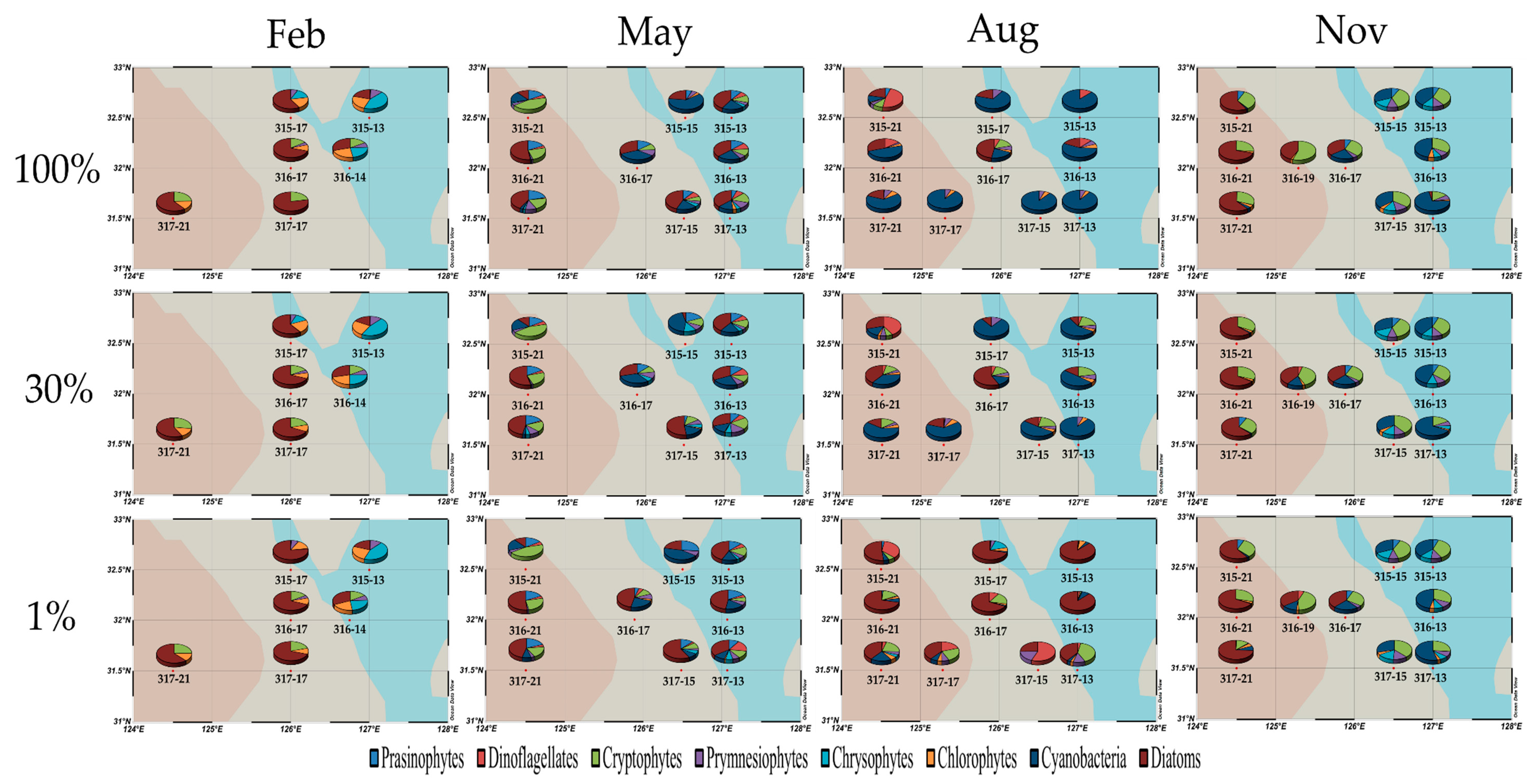
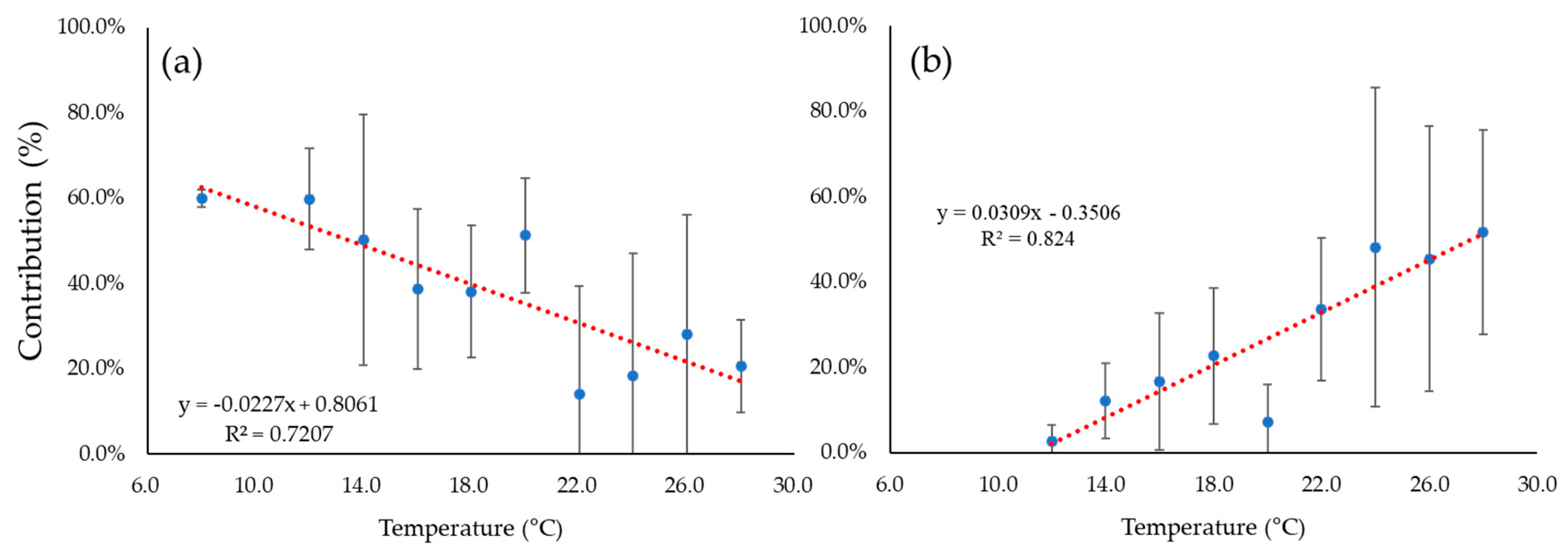
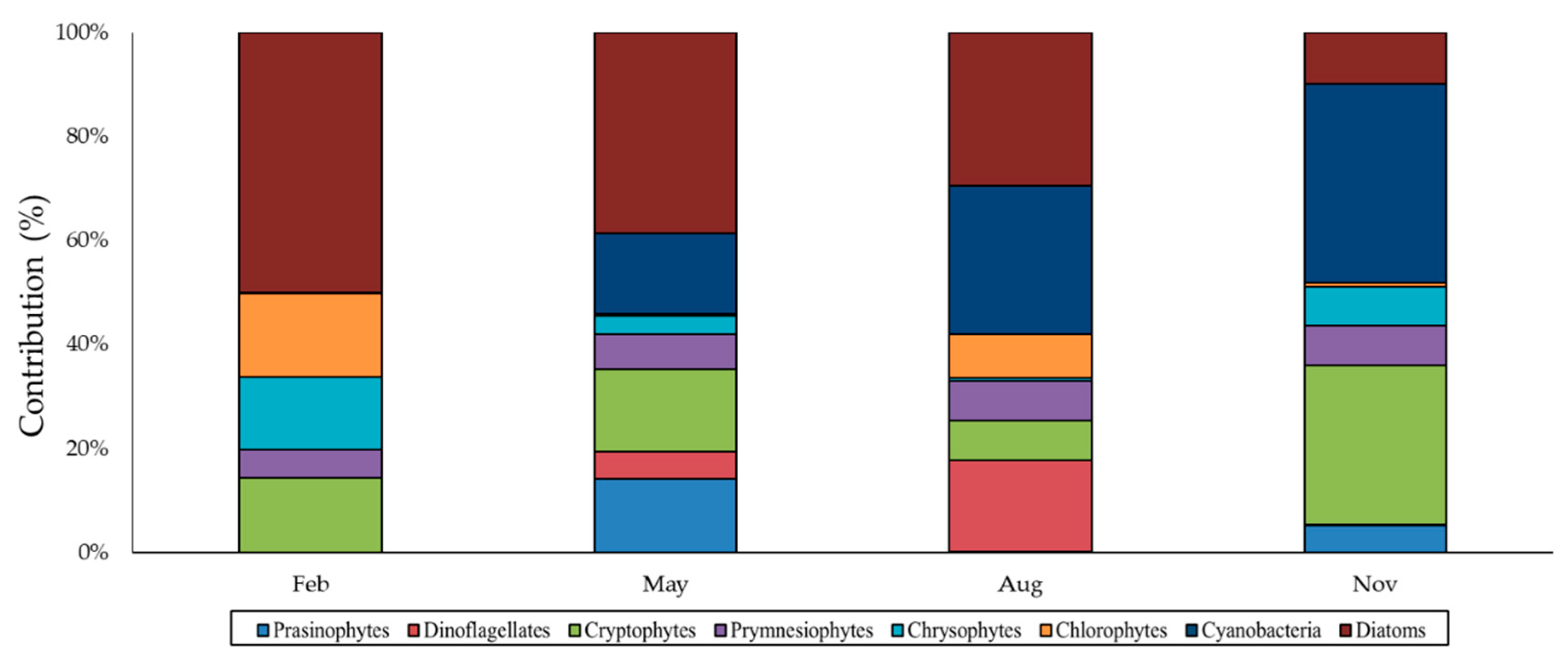
3.3. Phytoplankton Biomass and Community Structure

The monthly averaged chlorophyll-a concentration integrated from surface to 1% light depth was highest (35.2 ± 20.22 mg m−2) in May and lowest (5.2 ± 2.54 mg m−2) in February (Figure 3). In February, the integral chlorophyll-a concentration was relatively lower in the western part (2.8 mg m−2) compared to that in the eastern part (6.7 ± 2.46 mg m−2) of our study area, which is similar to the temperature distribution. In May, the integral chlorophyll-a concentration was highly variable across the study area with the range of 8.2–70.0 mg m−2 and the chlorophyll-a concentration was relatively higher in the southern part than in the northern part. In August, no distinct spatial distribution in the chlorophyll-a concentration was observed. In November, the spatial distribution in the integral chlorophyll-a concentration was opposite to that in August, which is similar to the nutrient distribution patterns (Table 2).
Generally, no distinct vertical differences in phytoplankton community compositions were observed at 100%, 30%, and 1% light depths for all the sampling seasons except August (Figure 4). The phytoplankton community compositions in August were conspicuously different between 30–100% light depths and 1% light depths. Cyanobacteria predominated, contributing 63.3% to the total phytoplankton biomass and diatoms were the second most abundant group (15.5%) at 100% light depths, whereas diatoms contributed 58.2% followed by dinoflagellates (13.0%) and other classes (<10%) at 1% light depths (Figure 4). Spatially, noticeable differences in phytoplankton community between the eastern and western parts were observed season, especially in November. Diatoms predominated in the western part, contributing 58.6% to the total phytoplankton biomass and cryptophytes were the second most abundant group (27.4%), whereas cyanobacteria predominated (45.0%) in the eastern part followed by cryptophytes (31.0%) in November. These two dominant groups were significantly (p < 0.01) correlated with water temperature (Figure 5). The contribution of diatoms was negatively related with water temperature (y = −0.0227x + 0.8061, r2 = 0.7207), whereas the contribution of cyanobacteria had a positive relationship with water temperature (y = 0.0309x − 0.3506, r2 = 0.824).
Overall, the major phytoplankton community in the study site was diatoms with a contribution more than 30% although it varied seasonally from 9.8% (November) and 50.0% (February) (Figure 6). Cyanobacteria were the second highest contributors ranging from 0% to 38.3% during our study period. Cyanobacteria were not appeared in February but their contribution increased steadily from May to November. The contributions of cryptophytes ranged from 7.8% to 30.7%. The contributions of prymnesiophytes were 5.4–7.6%, with a similar contribution for each cruise. Chlorophytes contributed 0.5–16.1%, with the highest contribution in February and were hardly observed in May and November (0.5% and 0.8%, respectively). Chrysophytes had the contributions of 0.6–14.0%, showing their highest contribution in February. Dinoflagellates showed their contributions of 0–17.4% and their highest contribution was in August. In the case of prasinophytes, they showed the contributions ranging from 0% to 14.2% and the highest contribution was in May (Figure 6).

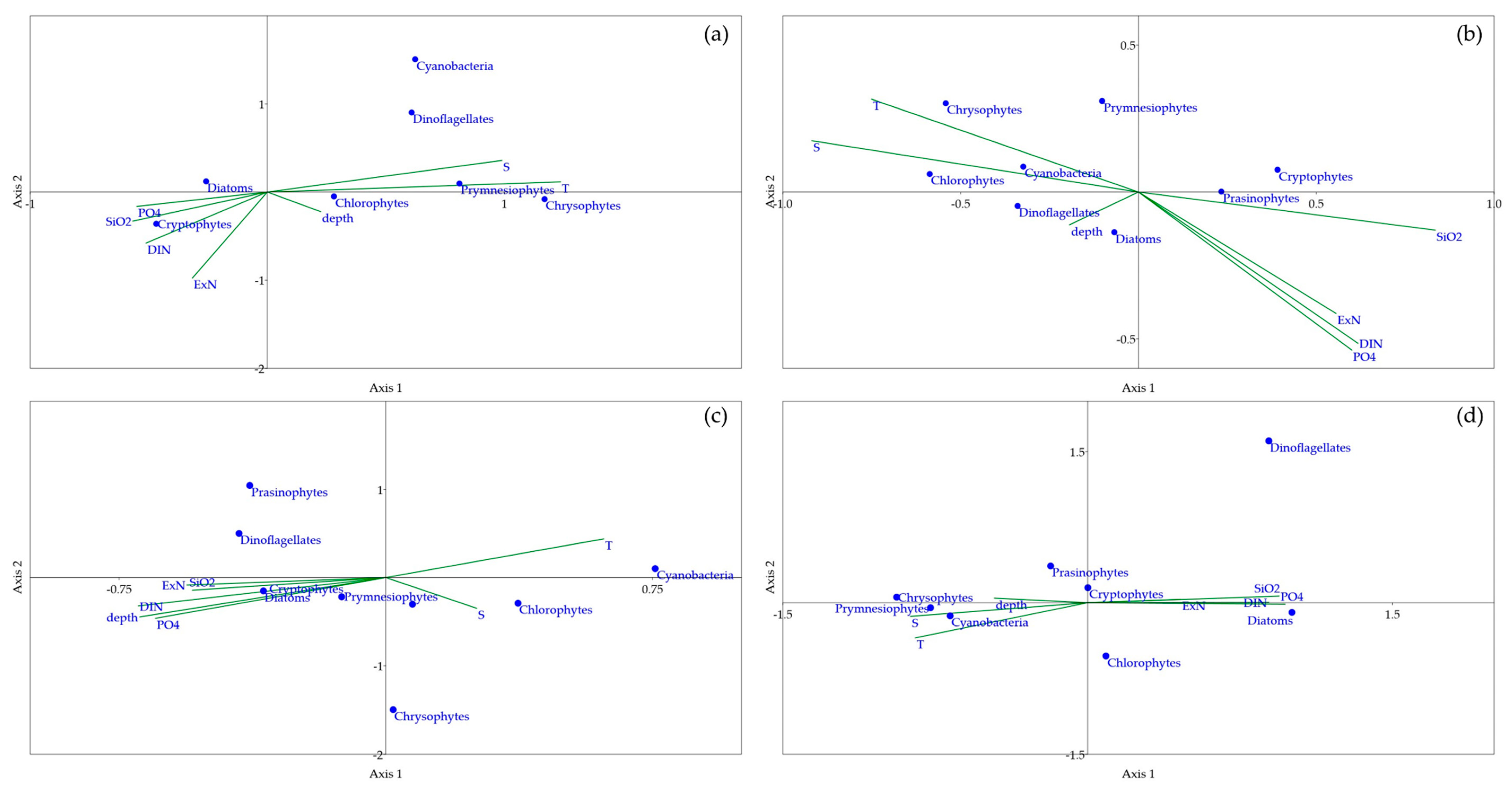
3.4. Canonical Correspondence Analysis (CCA)

CCA results between phytoplankton community and environmental parameters for each season are presented in Figure 7. In February, diatoms and chryptophytes showed negative correlations with temperature and salinity and positive correlations with nutrients, whereas chrysophytes and chlorophytes had positive correlations with temperature and salinity. In May, diatoms had no significant correlation with any environment parameter, whereas cyanobacteria and chrysophytes had negative correlations with nutrients and cyanobacteria had positive correlations with temperature and salinity. In August, cyanobacteria had a positive correlation with temperature and negative correlations with nutrients and depth. In comparison, diatoms had significantly positive correlations with nutrients and depth in August. Similarly, cyanobacteria showed a strong positive correlation with temperature and negative correlations with depth and nutrients in November. In comparison, diatoms had negative correlations with temperature and depth, and positive correlations with nutrients in November.

4. Discussion

The northern ECS is a typical temperate water seasonally affected mainly by four different water masses. The CDW, TCWW, KW, and YSCW, but their influence can vary seasonally [45,46]. Mixed waters were mainly distributed in our study area in February but YSCW was found at the most western stations (Sts. 315-21, 316-21, and 317-21) in May based on T-S diagrams. Low temperature, strong winds, and vigorous vertical mixing are generally observed in February during the Northeast Monsoon [47,48]. Weak surface stratification begins May and the water column was well stratified in August with TCWW mainly distributed at surface layer whereas the YSCW is mainly distributed at bottom layer (73 m). Normally, the surface layer in summer has a low density due to a high temperature and low salinity water from the CDW and the lower layer forms a strong stratification due to the distribution of the low temperature water from the YSCW and high salinity water from the TCWW [49]. In the northern ECS, the runoff from the Changjiang river is maximum in summer and minimum in winter [50]. According to a previous study, CDW is a main source of fresh water input in the ECS, increasing from spring to summer [51]. In November, the water masses were relatively well mixed (Figure 2).
In this study, we found that major inorganic nutrient concentrations were considerably higher in the western part compared to those in the eastern part in February and November during this study (Table 2), which is consistent with previous results [52]. The waters in the western part of the ECS are fully mixed from surface to the bottom because of the shallow water depth (<50 m), but in the eastern part vertical mixings occur only in the upper layer [35]. The noticeable vertical difference in nutrient concentrations were observed in August (Table 2) due to a strong stratified water column (Figure 2) which suppressed the upwelling of nutrients from the bottom layer. In addition, the seasonal average N:P ratios in the study area ranged from 10.5 to 422.9 (55.1 ± 64.6) which are higher than the Redfield ratio of 16 generally found in various oceans. [53] defined nutrient limitations following as; PO4 limitation when Si:P > 22 and DIN:P > 22; N limitation when DIN:P < 10 and Si:DIN > 1; Si limitation when Si:P < 10 and Si:DIN < 1. Various studies suggested that PO4 is a limiting nutrient to phytoplankton growth in the ECS [41,54,55,56]. This study also verified PO4-limited environmental conditions in May (124.5 ± 91.1) and August (50.3 ± 29.3) (Figure 8). According to [55] a high N:P ratio is related to very low PO4 concentration. Indeed, low PO4 concentrations (approximately 0.1 μM) were observed in May and August. These PO4-limited conditions could have caused the seasonal variation in phytoplankton community in the ECS. According to [57], Diatoms would have a higher phosphorus demand relative to other phytoplankton groups which may be reflected by lower N:P ratios in diatoms compared to those in other groups. Indeed, [43] showed the phytoplankton community in mid-shelf ECS in summer and identified 2 distinct phytoplankton communities under two major water masses with different nutrient conditions: PO4-rich Kuroshio intermediate water (KW) indicated by a low ExN value leading to diatom domination and PO4-limited CDW indicated by high ExN leading to small phytoplankton domination such as chlorophytes and cyanobacteria. However, we did not find the relationships in this study. In spring, diatoms were mostly dominant despite of PO4-limited water conditions. The PO4- limited condition in spring could be due to the spring bloom of diatoms, which is consistent with the results in Chesapeake Bay [58]. Even in our summer cruise period, opposite relationship between diatoms and ExN was observed. This discrepancy between this and previous studies could be caused by several factors. [42] observed pronounced effects of KW and CDW and a large range of PO4 concentration, whereas in this study, TCWW current was largely dominant rather than the KW and CDW and narrow range of PO4 concentration. In addition, the analysis in [42] was performed only in the surface layer, whereas this study was performed within the euphotic layer (surface to 1% light depth). Indeed, we also found a dominance of cyanobacteria in the surface layer with a lack of PO4 and diatoms dominant at the nutrient-rich depths as discussed in detail below.
The distinct vertical difference in dominant phytoplankton communities was observed in our study area in August with cyanobacteria predominated at surface layer and diatoms prevailed at deep layer. A strong water stratification appeared in the study area could have caused the vertical pattern of phytoplankton community [59]. A stratified water column restricts the upward supply of major inorganic nutrients to the upper euphotic surface layer. According to the resource competition theory [60,61,62], pico-phytoplankton are favored over larger phytoplankton in nutrient-limited conditions because of their higher nutrient affinity associated to their small size [63,64,65]. Thus, small size cyanobacteria are predominant in the nutrient-deficient surface layer in August. Since zeaxanthin is a marker pigment in cyanobacteria and plays an important role in protecting cyanobacteria against photoinhibition [66], the high concentration of zeaxanthin at surface might be due to much higher photosensitivity than that at the deep water column [67,68]. In addition, the water temperature was approximately 7 °C higher at surface than the deep layer in August. Indeed, CCA revealed a positive correlation between cyanobacteria and temperature in this study (Figure 7c). As water temperature exceeds 20 °C, the growth rates of eukaryotic phytoplankton usually stabilize or decrease whereas those of many cyanobacteria species increase because of their competitive advantage over high temperature [69,70,71]. Therefore, the water temperature and nutrient distribution in August had a great influence on the vertical distribution of phytoplankton communities.
During the four research periods, spatial difference in phytoplankton community was not significantly high, but in November, there was a clear difference in phytoplankton community between the western and eastern parts. The most predominant phytoplankton communities were diatoms in the western part and cyanobacteria in the eastern part. The cryptophytes were the third dominant species in both western and eastern parts. CCA result showed that cyanobacteria are associated with high temperature, high salinity, low nutrient concentrations, and depth, whereas diatoms are associated with low temperature and high nutrient concentrations in November (Figure 7d). Nutrient concentrations were also horizontally different, gradually decreasing toward the west. In relation to the distribution of these nutrients, zeaxanthin (major pigments of cyanobacteria) showed a negative correlation with nutrients (p < 0.01, t-test), whereas fucoxanthin (major pigments of diatoms) showed a positive correlation with nutrients (p < 0.01, t-test). These correlations with the nutrient concentrations indicate that nutrients are a major driver of the spatial difference in phytoplankton community distribution in November. Moreover, there was a significant difference in light condition based on the euphotic depths between in the western and eastern parts. The euphotic layer up to 1% depth was 43 m on average in the eastern part, whereas it was 7 m in the western part. Light can be a limiting factor largely influencing the spatial distribution of picophytoplankton, probably because the decreasing light in water is mostly variable in the water column [72,73]. According to [74], diatoms have high growth efficiency under a low light condition. In comparison to the phytoplankton community in the ECS, several studies in other oceanic basins influenced by large rivers were compared. Similar to the East China Sea, the Gulf of Mexico is a phosphate-limited environment during summer period [75,76]. These studies showed that diatoms generally predominate and cryptophytes are the second most abundant group in the winter and spring periods and cyanobacteria are most dominant during PO4-limited summer time compared to other seasons in the Gulf of Mexico. The spatiotemporal variations in the region are controlled mainly by river flow runoff, along with other environmental variables such as wind pressure and stratification [75,76]. In contrast, Western Tropical North Atlantic, which is a region largely affected by the Amazon River, is mainly dominated by the diatom-diazotroph associations (DDAs) [43]. In this region, the phytoplankton community structure and distributions are controlled by low concentrations of inorganic nitrite and nitrate (NO2 + NO3) [43].
Based on the four different seasonal observations in this study, the yearly average contributions of different phytoplankton communities were 32.0%, 20.6%, 17.2%, 6.9%, 6.4%, 6.4%, 5.7%, and 5.0% for diatoms, cyanobacteria, cryptophytes, prymnesiophytes, chlorophytes, chrysophytes, dinoflagellates, and prasinophytes, respectively, in the northern ECS. Chlorophyll-a concentrations were highest in May and lowest in February in this study which is consistent with previous results in the ECS [56,77]. Previous studies reported that diatoms are associated with phytoplankton blooms in early spring and that the dominant species in the ECS are mostly chain-forming diatoms such as Pseudonitzschia delicatissima, Thalassionema nitzschioides, and Paralia sulcate [28]. Consistent with previous observations, this study also verified that the dominant species were diatoms during the spring bloom in May.

5. Summary and Conclusions

There are multiple factors including light intensity, stability of water column, temperature, and nutrient conditions [78] that can cause variations in phytoplankton compositions and spatial distributions. The seasonal variations in the phytoplankton community were distinct in our study area although spatial and vertical variations were observed along the seasons. Diatoms appeared to be dominant in the northern ECS throughout the year in this study. Normally, diatoms are known to be competitive over other species at low water temperatures [79]. Therefore, in February with a low water temperature (Figure 2) and high nutrient concentrations (Table 2), diatoms were most predominated among our study periods. Moreover, diatoms are more efficient at high nutrient concentrations than small phytoplankton [80] and they can quickly respond to nutrient inputs [81]. Contrary to diatoms, cyanobacteria, as the next dominant species, started to appear in May and showed their contribution gradually increased from May to November in this study. According to previous research, water temperature is the main control factor for the distribution of cyanobacteria [82]. In this study, we also found that water temperature is a main factor driving the seasonal variation in the cyanobacteria contribution in the northern ECS throughout the year based on CCA result (Figure 7). Overall, the cyanobacteria contribution was strongly negatively correlated with the diatom contribution in the northern ECS during our study period in 2018 (Figure 6). This result implies an ecologically significant meaning for the marine ecosystem in the northern ECS. Under expected warming ocean scenarios, the potential change in dominant phytoplankton groups from diatoms to cyanobacteria could cause substantial differences in quantity and qualitative aspects of primary marine food sources in the northern ECS. Comprehensive monitoring for qualitative and quantitative characteristics of different phytoplankton communities is warrant for a better understanding their potential consequences on the entire marine ecosystem in the ECS.

Author Contributions

Conceptualization, Y.K., S.-H.Y., H.J.O., and S.H.L.; methodology, Y.K. and J.J.K.; validation, Y.K., S.-H.Y., and S.H.L.; formal analysis, Y.K.; investigation, J.J.K., J.H.L., D.L., K.K., H.K.J., and J.L.; data curation, Y.K.; writing—original draft preparation, Y.K.; writing—review and editing, Y.K., J.J.K., and S.H.L.; and visualization, Y.K. All authors have read and agreed to the published version of the manuscript.

Funding

This research was supported by the “Development of marine ecological forecasting system for Korean waters (R2018067)” funded by the National Institute of Fisheries Science (NIFS), Korea. This research also partly supported by a part of the project entitled “Construction of Ocean Research Station and their application” funded by the Ministry of Oceans and Fisheries, Korea.

Acknowledgments

We thank the anonymous reviewers who greatly improved an earlier version of manuscript.

Conflicts of Interest

The authors declare no conflict of interest.

References

  1. Smith, W., Jr.; Sakshaug, E. Polar Phytoplankton. In Polar Oceanography; Academic: San Diego, CA, USA, 1990; pp. 477–525. [Google Scholar]
  2. Sommer, U. The impact of light intensity and daylength on silicate and nitrate competition among marine phytoplankton. Limnol. Oceanogr. 1994, 39, 1680–1688. [Google Scholar] [CrossRef] [Green Version]
  3. Hilligsøe, K.M.; Richardson, K.; Bendtsen, J.; Sørensen, L.-L.; Nielsen, T.G.; Lyngsgaard, M.M. Linking phytoplankton community size composition with temperature, plankton food web structure and sea–air CO2 flux. Deep Sea Res. Part I 2011, 58, 826–838. [Google Scholar]
  4. Kilham, P.; Hecky, R.E. Comparative ecology of marine and freshwater phytoplankton 1. Limnol. Oceanogr. 1988, 33, 776–795. [Google Scholar] [CrossRef] [Green Version]
  5. Domingues, R.B.; Galvao, H. Phytoplankton and environmental variability in a dam regulated temperate estuary. Hydrobiologia 2007, 586, 117–134. [Google Scholar] [CrossRef]
  6. Wu, N.; Schmalz, B.; Fohrer, N. Development and testing of a phytoplankton index of biotic integrity (P-IBI) for a German lowland river. Ecol. Indic. 2012, 13, 158–167. [Google Scholar] [CrossRef]
  7. Smayda, T. Biogeographical meaning; indicators. In Phytoplankton Manual; UNESCO: Paris, France, 1978; pp. 225–229. [Google Scholar]
  8. Soares, M.C.S.; Lobão, L.M.; Vidal, L.O.; Oyma, N.P.; Barros, N.O.; Cardoso, S.J.; Roland, F. Light microscopy in aquatic ecology: Methods for plankton communities studies. Methods Mol. Biol. 2011, 689, 215–227. [Google Scholar]
  9. Chisholm, S.W.; Olson, R.J.; Zettler, E.R.; Goericke, R.; Waterbury, J.B.; Welschmeyer, N.A. A novel free-living prochlorophyte abundant in the oceanic euphotic zone. Nature 1988, 334, 340. [Google Scholar] [CrossRef]
  10. Gieskes, W.; Kraay, G. Dominance of Cryptophyceae during the phytoplankton spring bloom in the central North Sea detected by HPLC analysis of pigments. Mar. Biol. 1983, 75, 179–185. [Google Scholar] [CrossRef]
  11. Simon, N.; Barlow, R.G.; Marie, D.; Partensky, F.; Vaulot, D. Characterization of oceanic photosynthetic picoeukaryotes by flow cytometry. J. Phycol. 1994, 30, 922–935. [Google Scholar] [CrossRef]
  12. Readman, J.; Devilla, R.; Tarran, G.; Llewellyn, C.; Fileman, T.; Easton, A.; Burkill, P.; Mantoura, R. Flow cytometry and pigment analyses as tools to investigate the toxicity of herbicides to natural phytoplankton communities. Mar. Environ. Res. 2004, 58, 353–358. [Google Scholar] [CrossRef]
  13. Campbell, L.; Nolla, H.; Vaulot, D. The importance of Prochlorococcus to community structure in the central North Pacific Ocean. Limnol. Oceanogr. 1994, 39, 954–961. [Google Scholar] [CrossRef]
  14. Partensky, F.; Blanchot, J.; Lantoine, F.; Neveux, J.; Marie, D. Vertical structure of picophytoplankton at different trophic sites of the tropical northeastern Atlantic Ocean. Deep Sea Res. Part I 1996, 43, 1191–1213. [Google Scholar] [CrossRef]
  15. Wright, S.; Jeffrey, S.; Mantoura, R.; Llewellyn, C.; Bjørnland, T.; Repeta, D.; Welschmeyer, N. Improved HPLC method for the analysis of chlorophylls and carotenoids from marine phytoplankton. Mar. Ecol. Prog. Ser. 1991, 77, 183–196. [Google Scholar] [CrossRef]
  16. Mackey, M.; Mackey, D.; Higgins, H.; Wright, S. CHEMTAX-a program for estimating class abundances from chemical markers: Application to HPLC measurements of phytoplankton. Mar. Ecol. Prog. Ser. 1996, 144, 265–283. [Google Scholar] [CrossRef] [Green Version]
  17. Furuya, K.; Kurita, K.; Odate, T. Distribution of phytoplankton in the East China Sea in the winter of 1993. J. Oceanol. 1996, 52, 323–333. [Google Scholar] [CrossRef]
  18. Jiang, Y.-Z.; Cheng, J.-H.; Li, S.-F. Temporal changes in the fish community resulting from a summer fishing moratorium in the northern East China Sea. Mar. Ecol. Prog. Ser. 2009, 387, 265–273. [Google Scholar] [CrossRef]
  19. Chen, C.-T.A. Distributions of nutrients in the East China Sea and the South China Sea connection. J. Oceanol. 2008, 64, 737–751. [Google Scholar] [CrossRef]
  20. Moriyasu, S. The Tsushima Current. In Kuroshio, Its Physical Aspects; Stommel, H., Yoshida, K., Eds.; University of Tokyo Press: Tokyo, Japan, 1972; pp. 353–369. [Google Scholar]
  21. Nitani, H. Beginning of the Kuroshio. In Kuroshio Physical Aspect of the Japan Current; University of Washington Press: Seattle, WA, USA, 1972; pp. 129–163. [Google Scholar]
  22. Seung, Y. Water masses and circulations around Korean Peninsula. J. Oceanol. Soc. Korea 1992, 27, 324–331. [Google Scholar]
  23. Qilong, Z.; Xuechuan, W.; Yuling, Y. Analysis of water masses in the south Yellow Sea in spring. Oceanol. Limnol. Sin. 1996, 27, 42–428. (In Chinese) [Google Scholar]
  24. Zhou, M.-J.; Shen, Z.-L.; Yu, R.-C. Responses of a coastal phytoplankton community to increased nutrient input from the Changjiang (Yangtze) River. Cont. Shelf Res. 2008, 28, 1483–1489. [Google Scholar] [CrossRef]
  25. Guo, C.; Liu, H.; Zheng, L.; Song, S.; Chen, B.; Huang, B. Seasonal and spatial patterns of picophytoplankton growth, grazing and distribution in the East China Sea. Biogeosciences 2014, 11, 1847–1862. [Google Scholar] [CrossRef] [Green Version]
  26. Furuya, K.; Hayashi, M.; Yabushita, Y.; Ishikawa, A. Phytoplankton dynamics in the East China Sea in spring and summer as revealed by HPLC-derived pigment signatures. Deep Sea Res. Part II 2003, 50, 367–387. [Google Scholar] [CrossRef]
  27. Liu, X.; Xiao, W.; Landry, M.R.; Chiang, K.-P.; Wang, L.; Huang, B. Responses of phytoplankton communities to environmental variability in the East China Sea. Ecosystems 2016, 19, 832–849. [Google Scholar] [CrossRef]
  28. Guo, S.; Feng, Y.; Wang, L.; Dai, M.; Liu, Z.; Bai, Y.; Sun, J. Seasonal variation in the phytoplankton community of a continental-shelf sea: The East China Sea. Mar. Ecol. Prog. Ser. 2014, 516, 103–126. [Google Scholar] [CrossRef] [Green Version]
  29. Jiang, Z.; Chen, J.; Zhou, F.; Shou, L.; Chen, Q.; Tao, B.; Yan, X.; Wang, K. Controlling factors of summer phytoplankton community in the Changjiang (Yangtze River) Estuary and adjacent East China Sea shelf. Cont. Shelf Res. 2015, 101, 71–84. [Google Scholar] [CrossRef]
  30. Zhao, R.; Sun, J.; Bai, J. Phytoplankton assemblages in Yangtze River Estuary and its adjacent water in autumn 2006. Mar. Sci. 2010, 34, 32–39. [Google Scholar]
  31. He, Q.; Sun, J.; Luan, Q.-S.; Yu, Z.-M. Phytoplankton in Changjiang Estuary and adjacent waters in winter. Mar. Environ. Sci. 2009, 28, 360–365. [Google Scholar]
  32. Yoon, Y. Spatial distribution of phytoplankton community and red tide of dinoflagellate, Prorocentrum donghaience in the East China Sea during early summer. Korean J. Environ. Biol. 2003, 21, 132–141. [Google Scholar]
  33. Park, M.-O.; Kang, S.-W.; Lee, C.-I.; Choi, T.-S.; Lantoine, F. Structure of the phytoplanktonic communities in Jeju Strait and northern East China Sea and dinoflagellate blooms in spring 2004: Analysis of photosynthetic pigments. Sea 2008, 13, 27–41. [Google Scholar]
  34. Yoon, Y.-H.; Park, J.-S.; Soh, H.-Y.; Hwang, D.-J. On the marine environment and distribution of phytoplankton community in the northern East China Sea in early summer 2004. J. Korean Soc. Mar. Environ. Energy 2005, 8, 100–110. [Google Scholar]
  35. kim, D.; Choi, S.H.; Kim, K.H.; Shim, J.; Yoo, S.; Kim, C.H. Spatial and temporal variations in nutrient and chlorophyll-a concentrations in the northern East China Sea surrounding Cheju Island. Cont. Shelf Res. 2009, 29, 1426–1436. [Google Scholar] [CrossRef]
  36. Kang, J.J.; Lee, J.H.; Kim, H.C.; Lee, W.C.; Lee, D.; Jo, N.; Min, J.-O.; Lee, S.H. Monthly Variations of Phytoplankton Community in Geoje-Hansan Bay of the Southern Part of Korea Based on HPLC Pigment Analysis. J. Coast. Res. 2018, 85, 356–360. [Google Scholar] [CrossRef]
  37. Zapata, M.; Rodríguez, F.; Garrido, J.L. Separation of chlorophylls and carotenoids from marine phytoplankton: A new HPLC method using a reversed phase C8 column and pyridine-containing mobile phases. Mar. Ecol. Prog. Ser. 2000, 195, 29–45. [Google Scholar] [CrossRef] [Green Version]
  38. Lee, Y.-W.; Park, M.-O.; Im, Y.-S.; Kim, S.-S.; Kang, C.-K. Application of photosynthetic pigment analysis using a HPLC and CHEMTAX program to studies of phytoplankton community composition. Sea 2011, 16, 117–124. [Google Scholar] [CrossRef] [Green Version]
  39. Wolf, C.; Frickenhaus, S.; Kilias, E.S.; Peeken, I.; Metfies, K. Protist community composition in the Pacific sector of the Southern Ocean during austral summer 2010. Polar Biol. 2014, 37, 375–389. [Google Scholar] [CrossRef]
  40. Torrecilla, E.; Stramski, D.; Reynolds, R.A.; Millán-Núñez, E.; Piera, J. Cluster analysis of hyperspectral optical data for discriminating phytoplankton pigment assemblages in the open ocean. Remote Sens. Environ. 2011, 115, 2578–2593. [Google Scholar] [CrossRef] [Green Version]
  41. Wong, G.; Gong, G.; Liu, K.; Pai, S. ‘Excess nitrate’in the East China Sea. Estuar. Coast. Shelf Sci. 1998, 46, 411–418. [Google Scholar] [CrossRef] [Green Version]
  42. Xu, Q.; Sukigara, C.; Goes, J.I.; do Rosario Gomes, H.; Zhu, Y.; Wang, S.; Shen, A.; de Raús Maúre, E.; Matsuno, T.; Yuji, W. Interannual changes in summer phytoplankton community composition in relation to water mass variability in the East China Sea. J. Oceanol. 2019, 75, 61–79. [Google Scholar] [CrossRef]
  43. Goes, J.I.; do Rosario Gomes, H.; Chekalyuk, A.M.; Carpenter, E.J.; Montoya, J.P.; Coles, V.J.; Yager, P.L.; Berelson, W.M.; Capone, D.G.; Foster, R.A. Influence of the Amazon River discharge on the biogeography of phytoplankton communities in the western tropical north Atlantic. Prog. Oceanogr. 2014, 120, 29–40. [Google Scholar] [CrossRef] [Green Version]
  44. Ter Braak, C.J.; Smilauer, P. CANOCO Reference Manual and CanoDraw for Windows User’s Guide: Software for Canonical Community Ordination (Version 4.5); Microcomputer Power: Ithaca, NY, USA, 2002. [Google Scholar]
  45. Gong, G.-C.; Chen, Y.-L.L.; Liu, K.-K. Chemical hydrography and chlorophyll a distribution in the East China Sea in summer: Implications in nutrient dynamics. Cont. Shelf Res. 1996, 16, 1561–1590. [Google Scholar] [CrossRef]
  46. Chen, C.-T.A. Chemical and physical fronts in the Bohai, Yellow and East China seas. J. Mar. Sci. 2009, 78, 394–410. [Google Scholar] [CrossRef]
  47. Chen, C.; Beardsley, R.C.; Limeburner, R.; Kim, K. Comparison of winter and summer hydrographic observations in the Yellow and East China Seas and adjacent Kuroshio during 1986. Cont. Shelf Res. 1994, 14, 909–929. [Google Scholar] [CrossRef]
  48. Kusakabe, M. Hydrographic feature of the East China Sea. Bull. Coast. Oceanogr. 1998, 36, 5–17. [Google Scholar]
  49. Jang, S.-T.; Lee, J.-H.; Hong, C.-S. Mixing of Sea Waters in the Northern Part of the East China Sea in Summer. Sea 2007, 12, 390–399. [Google Scholar]
  50. Beardsley, R.; Limeburner, R.; Yu, H.; Cannon, G. Discharge of the Changjiang (Yangtze river) into the East China sea. Cont. Shelf Res. 1985, 4, 57–76. [Google Scholar] [CrossRef]
  51. Zuo-sheng, Y.; Milliman, J.D.; Fitzgerald, M.G. Transfer of water and sediment from the Yangtze River to the East China Sea, June 1980. Can. J. Fish. Aqua. Sci. 1983, 40, s72–s82. [Google Scholar] [CrossRef]
  52. Kim, D.; Shim, J.; Yoo, S. Seasonal variations in nutrients and chlorophyll-a concentrations in the northern East China Sea. Ocean Sci. J. 2006, 41, 125–137. [Google Scholar] [CrossRef]
  53. Justić, D.; Rabalais, N.N.; Turner, R.E.; Dortch, Q. Changes in nutrient structure of river-dominated coastal waters: Stoichiometric nutrient balance and its consequences. Estuar. Coast. Shelf Sci. 1995, 40, 339–356. [Google Scholar] [CrossRef]
  54. Harrison, P.; Hu, M.; Yang, Y.; Lu, X. Phosphate limitation in estuarine and coastal waters of China. J. Exp. Mar. Biol. Ecol. 1990, 140, 79–87. [Google Scholar] [CrossRef]
  55. Chen, Y.-L.L.; Lu, H.-B.; Shiah, F.-K.; Gong, G.; Liu, K.-K.; Kanda, J. New production and f-ratio on the continental shelf of the East China Sea: Comparisons between nitrate inputs from the subsurface Kuroshio Current and the Changjiang River. Estuar. Coast. Shelf Sci. 1999, 48, 59–75. [Google Scholar] [CrossRef]
  56. Gong, G.-C.; Wen, Y.-H.; Wang, B.-W.; Liu, G.-J. Seasonal variation of chlorophyll a concentration, primary production and environmental conditions in the subtropical East China Sea. Deep Sea Res. Part II 2003, 50, 1219–1236. [Google Scholar] [CrossRef]
  57. Hillebrand, H.; Steinert, G.; Boersma, M.; Malzahn, A.; Meunier, C.L.; Plum, C.; Ptacnik, R. Goldman revisited: Faster-growing phytoplankton has lower N: P and lower stoichiometric flexibility. Limnol. Oceanogr. 2013, 58, 2076–2088. [Google Scholar] [CrossRef]
  58. Li, J.; Glibert, P.M.; Zhou, M.; Lu, S.; Lu, D. Relationships between nitrogen and phosphorus forms and ratios and the development of dinoflagellate blooms in the East China Sea. Mar. Ecol. Prog. Ser. 2009, 383, 11–26. [Google Scholar] [CrossRef] [Green Version]
  59. Hampton, S.E.; Gray, D.K.; Izmest’eva, L.R.; Moore, M.V.; Ozersky, T. The rise and fall of plankton: Long-term changes in the vertical distribution of algae and grazers in Lake Baikal, Siberia. PLoS ONE 2014, 9, e88920. [Google Scholar] [CrossRef] [PubMed]
  60. Tilman, D. Resource competition between plankton algae: An experimental and theoretical approach. Ecology 1977, 58, 338–348. [Google Scholar] [CrossRef]
  61. Tilman, D. Resource Competition and Community Structure; Princeton University Press: Princeton, NJ, USA, 1982. [Google Scholar]
  62. Tilman, D.; Kilham, S.S.; Kilham, P. Phytoplankton community ecology: The role of limiting nutrients. Annu. Rev. Ecol. Syst. 1982, 13, 349–372. [Google Scholar] [CrossRef]
  63. Smith, R.E.; Kalff, J. Size dependence of growth rate, respiratory electron transport system activity and chemical composition in marine diatoms in the laboratory. J. Phycol. 1982, 18, 275–284. [Google Scholar] [CrossRef]
  64. Fogg, G.E. Review Lecture-Picoplankton. Proc. R. Soc. Lond. B Biol. Sci. 1986, 228, 1–30. [Google Scholar]
  65. Raven, J. The twelfth Tansley Lecture. Small is beautiful: The picophytoplankton. Funct. Ecol. 1998, 12, 503–513. [Google Scholar] [CrossRef]
  66. Demmig-Adams, B.; Adams, W.W.; Czygan, F.-C.; Schreiber, U.; Lange, O.L. Differences in the capacity for radiationless energy dissipation in the photochemical apparatus of green and blue-green algal lichens associated with differences in carotenoid composition. Planta 1990, 180, 582–589. [Google Scholar] [CrossRef]
  67. Descy, J.-P.; Sarmento, H.; Higgins, H.W. Variability of phytoplankton pigment ratios across aquatic environments. Eur. J. Phycol. 2009, 44, 319–330. [Google Scholar] [CrossRef]
  68. Claustre, H.; Kerhervé, P.; Marty, J.-C.; Prieur, L. Phytoplankton photoadaptation related to some frontal physical processes. J. Mar. Syst. 1994, 5, 251–265. [Google Scholar] [CrossRef]
  69. Mur, R.; Skulberg, O.; Utkilen, H. Cyanobacteria in the environment. In Toxic Cyanobacteria in Water; Chorus, I., Batram, J., Eds.; E&FN Spon: London, UK, 1999; pp. 15–40. [Google Scholar]
  70. Peperzak, L. Climate change and harmful algal blooms in the North Sea. Acta Oecol. 2003, 24, S139–S144. [Google Scholar] [CrossRef]
  71. Paerl, H.W.; Huisman, J. Climate change: A catalyst for global expansion of harmful cyanobacterial blooms. Environ. Microbiol. Rep. 2009, 1, 27–37. [Google Scholar] [CrossRef] [PubMed]
  72. Dusenberry, J.; Olson, R.; Chisholm, S. Field observations of oceanic mixed layer dynamics and picophytoplankton photoacclimation. J. Mar. Syst. 2000, 24, 221–232. [Google Scholar] [CrossRef]
  73. Moore, L.R.; Goericke, R.; Chisholm, S.W. Comparative physiology of Synechococcus and Prochlorococcus: Influence of light and temperature on growth, pigments, fluorescence and absorptive properties. Mar. Ecol. Prog. Ser. 1995, 116, 259–275. [Google Scholar] [CrossRef]
  74. Goldman, J.C.; McGillicuddy, D.J.J. Effect of large marine diatoms growing at low light on episodic new production. Limnol. Oceanogr. 2003, 48, 1176–1182. [Google Scholar] [CrossRef] [Green Version]
  75. Chakraborty, S.; Lohrenz, S.E. Phytoplankton community structure in the river-influenced continental margin of the northern Gulf of Mexico. Mar. Ecol. Prog. Ser. 2015, 521, 31–47. [Google Scholar] [CrossRef]
  76. Anglès, S.; Jordi, A.; Henrichs, D.W.; Campbell, L. Influence of coastal upwelling and river discharge on the phytoplankton community composition in the northwestern Gulf of Mexico. Prog. Oceanogr. 2019, 173, 26–36. [Google Scholar] [CrossRef]
  77. Shi, W.; Wang, M. Satellite views of the bohai sea, yellow sea, and East China Sea. Prog. Oceanogr. 2012, 104, 30–45. [Google Scholar] [CrossRef]
  78. Reid, P.; Lancelot, C.; Gieskes, W.; Hagmeier, E.; Weichart, G. Phytoplankton of the North Sea and its dynamics: A review. Neth. J. Sea Res. 1990, 26, 295–331. [Google Scholar] [CrossRef] [Green Version]
  79. Johnson, F.A. Green, bluegreen and diatom algae: Taxonomic differences in competitive ability for phosphorus, silicon and nitrogen. Arch. Hydrobiol. 1986, 106, 473485. [Google Scholar]
  80. Hassen, M.B.; Drira, Z.; Hamza, A.; Ayadi, H.; Akrout, F.; Issaoui, H. Summer phytoplankton pigments and community composition related to water mass properties in the Gulf of Gabes. Estuar. Coast. Shelf Sci. 2008, 77, 645–656. [Google Scholar] [CrossRef]
  81. Lagus, A.; Suomela, J.; Weithoff, G.; Heikkilä, K.; Helminen, H.; Sipura, J. Species-specific differences in phytoplankton responses to N and P enrichments and the N: P ratio in the Archipelago Sea, northern Baltic Sea. J. Plankton Res. 2004, 26, 779–798. [Google Scholar] [CrossRef] [Green Version]
  82. Kanoshina, I.; Lips, U.; Leppänen, J.-M. The influence of weather conditions (temperature and wind) on cyanobacterial bloom development in the Gulf of Finland (Baltic Sea). Harmful Algae 2003, 2, 29–41. [Google Scholar] [CrossRef]
Figure 1. Sampling stations in the northern East China Sea, 2018. The major currents in the northern East China Sea are based on [19].
Water 12 02695 g001
Figure 2. Vertical profiles of temperature and salinity in the northern East China Sea, 2018. (a) February, (b) May, (c) August, and (d) Nov for temperature; and (e) February, (f) May, (g) August, and (h) November for salinity.
Water 12 02695 g002
Figure 3. Horizontal distributions of water column-integrated chlorophyll-a concentration from surface to 1% light depth in the northern East China Sea (a) February, (b) May, (c) August, and (d) November.
Water 12 02695 g003
Figure 4. Seasonal distributions of phytoplankton communities at the euphotic depths (100%, 30%, and 1%) in the northern East China Sea, 2018.
Water 12 02695 g004
Figure 5. Relationships between contributions of two major phytoplankton communities and water temperature for all the cruise period, 2018. (a) Diatom (b) Cyanobacteria.
Water 12 02695 g005
Figure 6. Seasonal contributions of phytoplankton communities averaged from all the stations for each cruise period in the northern East China Sea, 2018.
Water 12 02695 g006
Figure 7. Canonical correspondence analysis of seasonal phytoplankton communities and environmental parameters measured at each cruise period in the northern East China Sea (a) February (b) May (c) August (d) November.
Water 12 02695 g007
Figure 8. Scatter diagrams of atomic nutrient ratios at the euphotic depths (100%, 30%, and 1%) in the northern East China Sea, 2018.
Water 12 02695 g008
Table 1. Description of sampling stations in the northern East China Sea for each cruise period, 2018.
DateStationLatitudeLongitudeEuphotic Depth (m)
February315-1332.5127.019
315-1732.5125.95
316-1432.0126.819
316-1732.0125.914
317-1731.5125.919
317-2131.5124.55
May315-1332.5127.027
315-1532.5126.538
315-2132.5124.511
316-1332127.027
316-1732125.927
316-2132124.55
317-1331.5127.016
317-1531.5126.533
317-2131.5124.514
August315-1332.5127.041
315-1732.5125.946
315-2132.5124.522
316-1332127.041
316-1732125.927
316-2132124.530
317-1331.5127.035
317-1531.5126.554
317-1931.5125.335
317-2131.5124.519
October315-1332.5127.041
315-1532.5126.541
315-2132.5124.58
316-1332127.033
316-1732125.927
316-1932125.38
316-2132124.55
317-1331.5127.049
317-1531.5126.549
317-2131.5124.55
Table 2. The dissolved inorganic nutrient concentrations (μM) at the euphotic depths (100%, 30%, and 1%) of water column in the northern East China Sea, 2018.
StationLight (%)NH4NO2NO3DINPO4SiO2
February315-13100%0.840.404.816.040.337.15
30%0.920.364.015.290.296.27
1%1.010.395.076.480.327.11
315-17100%0.800.1010.6611.560.6013.67
30%0.930.085.076.080.336.79
1%0.900.084.925.900.358.07
316-14100%0.930.098.319.330.338.76
30%0.910.097.958.950.358.65
1%0.910.108.069.070.338.50
316-17100%0.850.285.106.230.296.96
30%0.730.274.795.780.296.83
1%1.050.244.665.950.296.60
317-17100%1.010.187.879.070.419.82
30%0.800.155.246.190.346.04
1%0.790.117.808.700.419.97
317-21100%0.810.0911.5512.460.5314.46
30%0.780.1012.3413.220.6115.37
1%0.820.1013.1914.110.6016.77
average0.880.187.308.360.399.32
S.D0.090.112.942.840.113.40
May315-13100%1.58 0.09 1.98 3.66 0.02 3.45
30%1.51 0.05 1.17 2.74 0.02 3.44
1%1.56 0.06 1.31 2.93 0.02 4.68
315-15100%1.59 0.06 3.23 4.88 0.03 3.99
30%1.49 0.04 1.43 2.95 0.02 4.11
1%1.56 0.05 1.29 2.89 0.04 4.59
315-21100%1.64 0.23 4.47 6.34 0.11 11.36
30%1.65 0.21 3.68 5.54 0.13 11.54
1%1.52 0.16 3.51 5.19 0.08 10.68
316-13100%1.96 0.07 3.43 5.46 0.03 5.78
30%1.60 0.05 1.04 2.68 0.02 4.36
1%1.77 0.19 4.51 6.47 0.18 6.91
316-17100%2.14 0.06 1.41 3.61 0.03 6.64
30%1.61 0.07 1.11 2.79 0.04 7.15
1%1.54 0.04 1.30 2.88 0.03 6.59
316-21100%1.53 0.51 10.23 12.26 0.33 9.86
30%1.44 0.48 8.90 10.82 0.30 9.50
1%1.47 0.44 7.51 9.43 0.30 7.83
317-13100%2.65 0.30 1.69 4.64 0.03 3.72
30%1.55 0.06 1.06 2.66 0.01 5.95
1%1.60 0.06 0.85 2.51 0.01 5.52
317-15100%1.55 0.05 1.27 2.86 0.01 3.89
30%1.57 0.05 1.01 2.63 0.01 3.97
1%1.57 0.26 2.61 4.44 0.10 6.03
317-21100%2.06 0.10 2.61 4.78 0.01 8.87
30%1.72 0.08 1.45 3.26 0.01 9.58
1%1.58 0.45 8.12 10.16 0.31 12.41
average1.670.163.044.870.086.75
S.D0.260.152.662.760.102.79
StationLight (%)NH4NO2NO3DINPO4SiO2
August315-13100%0.41 0.06 1.49 1.97 0.06 8.31
30%0.41 0.09 1.99 2.50 0.06 7.94
1%0.44 0.09 14.14 14.67 0.53 13.75
315-17100%1.46 0.09 1.41 2.97 0.07 8.48
30%0.40 0.05 1.16 1.61 0.05 8.62
1%0.36 0.09 8.45 8.90 0.49 10.75
315-21100%0.80 0.14 2.18 3.13 0.07 7.07
30%0.80 0.11 2.00 2.92 0.07 6.91
1%1.17 1.66 5.68 8.51 0.11 11.79
316-13100%0.54 0.06 2.04 2.63 0.03 8.29
30%2.76 0.07 0.96 3.78 0.03 3.31
1%0.43 0.06 9.11 9.59 0.42 8.88
316-17100%0.72 0.20 2.96 3.88 0.08 2.61
30%0.61 0.17 3.05 3.83 0.05 2.70
1%0.74 0.29 13.84 14.86 0.34 14.71
316-21100%1.29 0.05 1.54 2.88 0.06 2.10
30%0.56 0.06 1.68 2.31 0.07 2.74
1%0.74 1.26 4.06 6.06 0.18 7.80
317-13100%0.58 0.04 3.35 3.96 0.06 5.45
30%3.15 0.04 0.79 3.98 0.03 2.11
1%0.49 0.45 10.73 11.67 0.28 11.89
317-15100%1.30 0.06 1.56 2.93 0.06 3.59
30%1.02 0.06 1.96 3.04 0.09 4.12
1%3.71 0.06 9.46 13.23 0.43 9.97
317-19100%0.67 0.05 1.63 2.35 0.05 2.12
30%0.64 0.05 1.85 2.54 0.05 2.59
1%1.11 0.69 6.50 8.30 0.15 8.53
317-21100%1.54 0.04 1.16 2.74 0.06 2.38
30%0.40 0.04 1.68 2.11 0.06 3.73
1%0.56 0.10 2.30 2.96 0.08 3.81
average0.990.214.025.230.146.57
S.D0.830.373.884.000.153.76
October315-13100%0.660.151.792.610.182.72
30%0.740.101.382.220.131.99
1%0.790.141.182.110.172.32
315-15100%0.490.482.663.620.223.71
30%0.630.401.882.900.173.09
1%0.730.472.323.510.233.63
315-21100%2.070.1313.7315.930.5613.36
30%0.700.1110.3511.160.5715.78
1%0.620.1210.9111.650.5614.81
316-13100%1.040.212.423.670.192.66
30%0.600.071.932.600.102.79
1%0.740.111.412.270.172.35
316-17100%0.600.495.386.470.367.99
30%0.540.524.625.680.397.44
1%0.600.544.345.490.416.93
316-19100%1.240.148.7010.070.4911.69
30%0.780.129.2810.180.4712.39
1%0.560.117.798.470.5010.50
316-21100%0.870.076.307.240.478.25
30%0.750.118.299.150.5910.99
1%0.890.119.2810.280.5512.24
317-13100%1.100.184.746.020.222.84
30%0.660.091.812.550.172.35
1%0.710.111.472.290.222.13
317-15100%0.880.162.273.300.222.99
30%0.850.151.902.900.212.91
1%1.390.212.003.600.233.04
317-21100%1.050.149.2310.410.5111.52
30%0.650.128.168.930.5310.68
1%0.650.128.709.480.5111.18
average0.820.205.216.220.346.91
S.D0.320.153.673.750.174.59

