Flood Risk Analysis of Different Climatic Phenomena during Flood Season Based on Copula-Based Bayesian Network Method: A Case Study of Taihu Basin, China

Abstract

We propose a flood risk management model for the Taihu Basin, China, that considers the spatial and temporal differences of flood risk caused by the different climatic phenomena. In terms of time, the probability distribution of climatic phenomenon occurrence time was used to divide the flood season into plum rain and the typhoon periods. In terms of space, the Taihu Basin was divided into different sub-regions by the Copula functions. Finally, we constructed a flood risk management model using the Copula-based Bayesian network to analyze the flood risk. The results showed the plum rain period occurs from June 24 to July 21 and the typhoon period from July 22 to September 22. Considering the joint distribution of sub-region precipitation and the water level of Taihu Lake, we divided the Taihu Basin into three sub-regions (P-I, P-II, and P-III) for risk analysis in the plum rain period. However, the Taihu Basin was used as a whole for flood risk analysis in the typhoon period. Risk analysis indicated a probability of 2.4%, and 0.8%, respectively, for future adverse drainage during the plum rain period and the typhoon period, the flood risk increases rapidly with the rising water level in the Taihu Lake.

1. Introduction

Flood risk management includes flood risk analysis [1,2,3], vulnerability analysis [4,5,6], flood disaster assessment [7,8,9,10], and response [11,12,13]. Several factors can influence the risk of flood disasters, such as astronomy, meteorology, hydrology, topography, landforms, and human activities. Obviously, the interaction between such heterogeneous factors cannot be described clearly by using only one variable and, therefore, the study of multivariable joint distribution models is a significant facet of research on flood risk analysis [14,15].

Multivariable joint distribution models can be divided into two types [16] based on the characteristics of marginal distribution functions. There are models with the same marginal distributions (such as the multivariate normal model) [17,18,19] and models with different marginal distributions (such as the meta-Gaussian model) [20,21,22]. Considering the actual situation of a flood disaster, the second type of model is more appropriate, as choosing marginal distributions is more flexible. However, the requirement of correlation between variables in some models (such as the Farlie-Gumbel-Morgenstern model [20]) limit the application range of such models. Consequently, the copula function, that has a more flexible structure, has been introduced in flood risk analysis. Then, researchers study the various aspects of the copula function, such as function type selection, parameter estimation, and the goodness-of-fit [23,24,25,26]. In hydrology, the application of copula function, generally, includes several parts, which are as follows: (1) frequency analysis of hydro-meteorological variables that have multi-feature attributes, such as flood duration, flood volume, and flood peaks [27,28]; (2) the encountering combination problem of different hydrological extreme events, such as an interval rainstorm combined with river flooding [23,24,29]; and (3) bias correction techniques, that are used generally in climate and hydrological modeling [30,31,32]. The study of flood risk analysis involves all these aspects.

Under the influence of different climatic phenomena, the types of precipitation in the Taihu Basin are divided into plum rain and typhoon rain. Statistical data indicate that the duration of the plum rain differs each year, with the average being approximately 20 days. Generally, the plum rain period starts in the middle of June, and ends in early July. Mid-May is the earliest month when the typhoon rains starts to affect the Taihu Basin, with the latest being middle November. However, most typhoons occur between July and September and, particularly, between late August and early September.

The different types of precipitation bring about spatial and temporal differences in flood risk, which leads to significant challenges in flood management in the basin. Hu et al. [33] constructed the joint distribution functions of typhoon and plum rain with the Gumbel copula function and pointed out that the encounter probability of typhoon and plum rain is 9.23% in the Taihu Basin. Taking into account a particular typhoon’s birthplace, movement path, and rainfall characteristics, Cui et al. [34] put forward a concept of typhoon impacting the Taihu Basin. This concept points out that there are three kinds of typhoon which could affect the Taihu basin. It is useful information for typhoon emergency management. Liu et al. [28] used the Frank copula function to study the correlation between the start time of the plum rain period and the rainfall amounts of this period in the Taihu Basin. The results showed that when the plum rain period started early, more attention would need to be paid to flooding.

The above-mentioned studies mainly estimate the hydrological variables encountering combination problems, and they focus on the entire flood season [25,35,36]. However, compared with other situations, the encountering probability of hydrologically extreme events is small, as shown in previous study results. For example, in the Taihu Basin, the probability of only plum rain arising or only a typhoon occurring is 90.77%, compared with the occurance of plum rain and typhoons [33]. Accordingly, the primary objectives of this research are; (1) to analyze the temporal characteristics of plum rain and typhoons in the research areas and to divide the flood season into the plum rain period and the typhoon period; (2) to study the precipitation heterogeneous in different climatic phenomena and identify the flood risk during the different periods; and (3) to build a proper copula-based Bayesian network model for flood control in the Taihu Basin.

2. Study Area and Data

2.1. Study Area

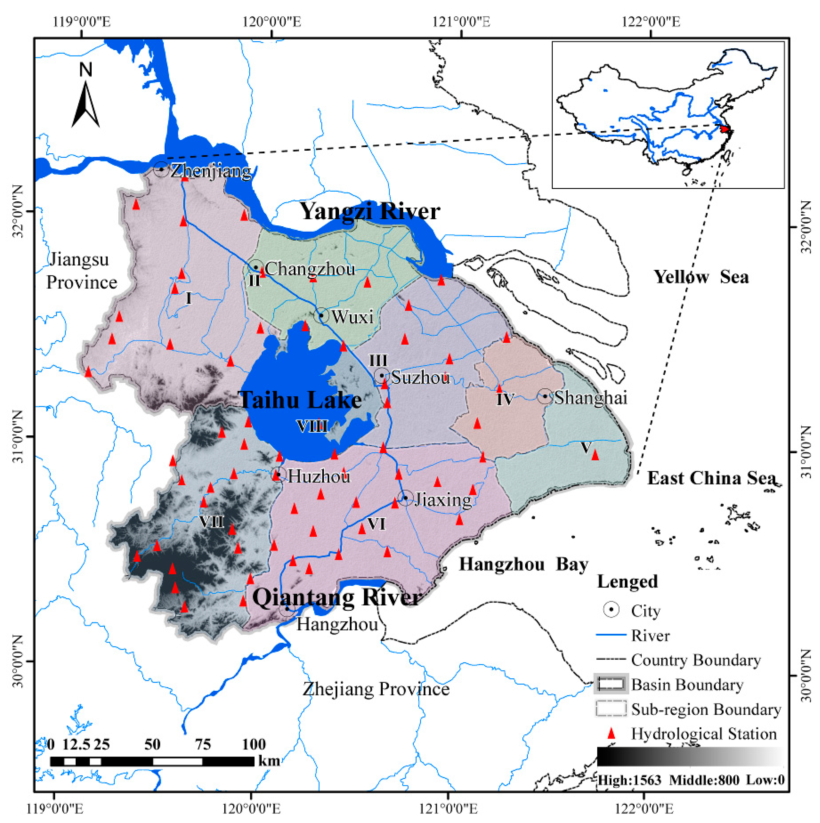
As shown in Figure 1, the Taihu Basin is located in the delta region of the Yangtze River of China. The total area of the Taihu Basin is approximately 36,895 km². The Taihu Lake, with a water surface area of 2336.8 km², is located in the center of the basin. The basin lies in a subtropical zone, with the climate being controlled by the summer monsoon. The average annual precipitation is 1177 mm, concentrated mainly in the flood season. The upper reaches of the Taihu Basin are mountainous areas, whereas the lower reaches are mostly plains. In the flood season, this unusual terrain (high on all sides and low in the middle) leads to upstream floods and basin precipitation confluence in the plains (urbanized areas). Consequently, flood disasters can occur easily. According to geographic and hydrological conditions, the Taihu Basin is usually divided into eight hydrological regions [36]. Detailed information on the eight hydrological sub-regions is listed in

Table 1. Information on eight hydrological sub-regions.

ID	Name	Areas	Annual Precipitation
I	Hu Xi	7897 km2	1169.1 mm
II	Wu Cheng Xi Yu	3615 km2	1118.5 mm
III	Yang Cheng Dian Mao	4314 km2	1142.0 mm
IV	Pu Xi	2165 km2	1159.9 mm
V	Pu Dong	2301 km2	1153.2 mm
VI	Hang Jia Hu	7480 km2	1247.0 mm
VII	Zhe Xi	5931 km2	1430.4 mm
VIII	Taihu Lake	3192 km2	1183.4 mm

.

2.2. Data

Plum rain data and daily Taihu Lake water level data, from 1962 to 2011, were obtained from the Taihu Basin Authority of Ministry of Water Resources (TBA). The daily precipitation data of 67 hydrological stations, from 1962 to 2011, were also provided by the TBA. Typhoon data from 1962 to 2011 were derived from the basic data sets of Northern Pacific typhoons in Shanghai Typhoon Institute, China Meteorological Administration.

3. Methodology

3.1. Flood Season Staging Based on the Different Climatic Phenomena

Under the influence of continental polar air masses, maritime tropical air masses, and tropical cyclones, the precipitation in the Taihu Basin include, plum rain and typhoon rain. The flood season can be divided into the plum rain period and the typhoon period according to the climatic phenomenon occurrence times. The intensity of rainfall is small in the plum rain period but the duration is long, whereas, during the typhoon period, the rainfall intensity is larger and the duration is short. Precipitation with such varying characteristics obviously leads to differing flood risks, as well as significant challenges to flood management in the basin.

3.1.1. Distribution Function of Plum Rain and Typhoon Occurrence Times

The start time of the plum rain period (STP) and end time of the plum rain period (ETP) and the initial time when typhoon begins to affect the Taihu Basin (ITT) were chosen as indices to describe the occurrence time rule of plum rain, and typhoon, respectively. Norm distribution, Log-norm distribution, Gamma distribution, Beta distribution, Logistics distribution, and Weibull distribution, the six distribution functions commonly used in hydrology and meteorology, were chosen as candidate functions, and the maximum likelihood method was used for parameter estimation. The Kolmogorov-Smirnov (K-S) goodness-of-fit hypothesis test was applied to test the six distribution functions. In addition, the Probability Point Correlation Coefficient (PPCC), Root Mean Square Error (RMSE), Mean Absolute Error (MAE), and the Deterministic Coefficient (DC) were used to determine the most suitable probability density function (PDF) and cumulative distribution function (CDF) for relevant random variables (STP, ETP, and ITT). The definition of each test method is as follows:

$$\mathrm{PPCC}=\frac{{\displaystyle \sum _{i=1}^n(x_i-\overline{x})(y_i-\overline{y})}}{\sqrt{{\displaystyle \sum _{i=1}^n{(x_i-\overline{x})}^2}{\displaystyle \sum _{i=1}^n{(y_i-\overline{y})}^2}}}$$

(1)

$$\mathrm{RMSE}=\frac{1}{n}\sqrt{{\displaystyle \sum _{i=1}^n{(x_i-y_i)}^2}}$$

(2)

$$\mathrm{MAE}=\frac{1}{n}{\displaystyle \sum _{i=1}^n\left|x_i-y_i\right|}$$

(3)

$$\mathrm{DC}=1-\frac{{\displaystyle \sum _{i=1}^n{(x_i-y_i)}^2}}{{\displaystyle \sum _{i=1}^n{(x_i-\overline{x})}^2}}$$

(4)

where x_i and y_i represent the empirical frequency, and theoretical frequency, respectively; $\overline{x}$ and $\overline{y}$ are the mean of empirical frequency and theoretical frequency, respectively; and n is the number of samples.

3.1.2. Flood Season Staging and Results Verification

We chose the point-in-time when the STP cumulative is 90% as the starting point of the plum rain period, and the point-in-time when the ITT cumulative distribution is 90%, as the end time of the typhoon period (the 90% percentile is the closest to the actual situation). The coefficient ω was proposed to calculate the time when the plum rain period ended and the typhoon period started. We determined the time node of the demarcation point between the plum rain period and the typhoon period using this coefficient. The time node with the maximum ω value was chosen. The coefficient ω can be calculated as follows:

$$\omega =F_{(x)}^{{}_{plum}}\times (1-F_{(x)}^{{}_{typhoon}})$$

(5)

where ω represents the contribution rate of plum rain and typhoon to precipitation, $F_{\left(x\right)}^{plum}$ is the CDF of the ETP, and $F_{\left(x\right)}^{typhoon}$ is the CDF of the ITT.

The flood season staging results were tested against the Taihu Lake water level, which is the response factor of precipitation. Considering the actual situation, we chose the mixture normal distribution to fit the time when the water level of the Taihu Lake exceeds the warning water level (TWL). The warning water level of Taihu Lake is 3.8 m (according to the flood control project of the Taihu Basin [37]). The mixture normal distribution definition is as follows:

$$X~{\alpha }_{1}N({\mu }_1,{\sigma }_1{}^2)+{\alpha }_{2}N({\mu }_2,{\sigma }_2{}^2)$$

(6)

where α₁ and α₂ are the weight coefficients (α₁ + α₂ = 1), μ₁ and μ₂ are the means of the samples, and σ₁ and σ₂ are the mean square deviations of the samples.

3.2. Division of Precipitation Sub-Region Based on Hydrological Regionalization

Optimal division of the precipitation sub-regions was carried out in two steps, namely; (1) clustering of the hydrological sub-region, and (2) selection of the optimal precipitation sub-region division. The first step is based on the division of eight sub-regions (I, II, III, IV, V, VI, VII, VIII), which is the result of hydrological regionalization. In any hydrological sub-region, the geographical and hydrological conditions are the same, and the construction and planning of the water conservancy projects are mutually compatible. However, the different hydrological sub-regions can have similar precipitation characteristics. To respectively divide the precipitation sub-regions in the plum rain period and the typhoon period, correlation analysis methods were used. The second step is based on the relationship of regional precipitation and the Taihu Lake water level, which plays a significant role in flood control. The Copula functions were applied in the selection of optimal precipitation sub-regions division. This method not only maintains the hydraulic connection between the sub-regions, but also considers the spatial distribution of precipitation.

3.2.1. Clustering of Hydrological Sub-Regions Based on the Correlation Analysis of Precipitation

First, the Thiessen polygon method was used to calculate precipitations of the eight sub-regions during the plum rain and typhoon periods. Next, Person correlation, Spearman correlation, Kendall correlation, which are the three correlation analysis methods generally used in hydrology and meteorology assessments, were chosen to analyze the precipitation correlation between each sub-region. Finally, the sub-regions with strong precipitation correlations were merged successively.

3.2.2. Select Optimal Precipitation Sub-Regions Division by Copula Functions

The optimal precipitation sub-region division, which best reflects the relationship between precipitation and water level, was selected using Copulas. Copulas are defined as multivariate distribution functions with uniform margins on the interval 0 to 1. Based on Sklar’s theorem [38], copulas are capable of linking the joint CDF to its marginal distribution functions [39].

The joint distribution of sub-region precipitations and the Taihu Lake water level can be expressed by a copula as follows:

$$H(x_1,x_2,\cdots ,x_n,y)=C_{\theta }(F_1(x_1),F_2(x_2),\cdots ,F_n(x_n),F(y))$$

(7)

where H is a joint distribution, n is the number of precipitation sub-region, F_i(x_i) represents the marginal distribution of the i-th sub-region precipitation, F(y) represents the marginal distribution of the Taihu Lake water level, and C_θ is the copula CDF with parameter θ.

We selected four widely used Archimedean copulas (Clayton, Gumbel, Frank, and Joe copulas) as the candidate functions to model the joint distribution of regional precipitation and the Taihu Lake water level. The four Archimedean copula functions are defined in

Table 2. Function expressions of Archimedean copulas.

Family	Parameter Space θ	Generator $\mathit{\phi }(\mathit{t})$	Expression $\mathit{C}({\mathit{u}}_1,{\mathit{u}}_2,\cdots ,{\mathit{u}}_{\mathit{d}})$
Clayton	[0, ∞)	$\frac{1}{\theta }(t^{-\theta }-1)$	${\left[({\displaystyle \sum _{j=1}^d{u}_j^{-\theta }})+1-d\right]}^{-\frac{1}{\theta }}$
Gumbel	[1, ∞)	${(-\ln t)}^{\theta }$	$\exp \left\{-{\left[{\displaystyle \sum _{j=1}^d{(-\ln u_j)}^{\theta }}\right]}^{\frac{1}{\theta }}\right\}$
Frank	[0, ∞)	$-\ln \frac{e^{-\theta t}-1}{e^{-\theta }-1}$	$-\frac{1}{\theta }\ln \left[1+({\displaystyle \prod _{j=1}^d{e}^{-\theta u_j}}-1)/{(e^{-\theta }-1)}^{d-1}\right]$
Joe	[1, ∞)	$-\ln (1-{(1-t)}^{\theta })$	$1-{\left\{1-{\displaystyle \prod _{j=1}^d\left[1-{(1-u_j)}^{\theta }\right]}\right\}}^{\frac{1}{\theta }}$

NOTES: $u_1,u_2,\cdots ,u_d$ are independent uniform distributions.

[39].

Estimating parameter θ of the Archimedean copulas can be done by using different parametric and semi-parametric methods, such as Kendall’s τ method, Spearman’s ρ method and maximum likelihood-based methods (MLs). MLs include the full maximum likelihood method (FML), the inference for margins method (IFM), and the canonical maximum likelihood method (CML). We used the IFM for parameter estimation [40,41].

Several commonly evaluation criteria were used to select the optimal copula functions [42], such as the Akaike Information Criterion (AIC) and the Bayesian Information Criterion (BIC). The definition of the evaluation criteria are as follows:

$$\mathrm{AIC}=-2\ln (L)+2k$$

(8)

$$\mathrm{BIC}=-2\ln (L)+k\ln (n)$$

(9)

where L is the likelihood function, k is the number of joint distribution function parameters, and n is the number of samples.

The optimal precipitation sub-region division of the plum rain period and the typhoon period were determined by comparative analysis of the relationship between sub-region precipitations and the Taihu Lake water level under different hydrological sub-region clustering situations.

3.3. Flood Risk Management Based on Copula-Based Bayesian Network

Based on a posterior knowledge input, the backward reasoning function of the Bayesian network was utilized to conduct simulation calculations of the water level states in some certain precipitation situations that could occur in future during the plum rain and the typhoon periods [43,44].

3.3.1. Setting of Flood Disaster Situations

The flood control planning of the Taihu Basin indicates that, the flood control standards of the basin and sub-regions are 100, and 50 years, respectively after 2025. The warning water level of Taihu Lake is 3.8 m and the water level with safety guarantee of the Taihu Lake is 4.65 meters [37]. The results of the precipitation sub-region division indicated two categories, namely: (1) the spatial distribution of precipitation of the entire basin is assumed homogeneous; therefore, we chose the basin flood control standard, the warning water level, and the water level with safety guarantee of Taihu Lake to design the flood disaster situation; (2) dividing the precipitation of the basin into different regions indicates that the spatial distribution of precipitation is heterogeneous; therefore, the flood control standards of those sub-regions and the warning water level of Taihu Lake should be used to design the flood disaster situation.

3.3.2. Establishment of Bayesian Network

Bayesian networks are probabilistic models that describe the conditional dependencies of a set of random variables by means of directed acyclic graphs (DAG) [45]. The joint density for Bayesian networks can be expressed as follows: [46,47,48]

$$f_{X_1,\cdots ,X_n}(x_1,\cdots ,x_n)={\displaystyle \prod _{i=1}^n{f}_{X_{i}P\mathrm{a}(X_i)}(x_i{X}_{P\mathrm{a}(X_i)}=x)}$$

(10)

where X_Pa(Xi) = x is a shorthand notation for X_Pa1(Xi) = x_Pa1(Xi), … , X_Pam(Xi) = x_Pam(Xi) and Pa(X_i) indicate the set containing m parents of node X_i. For nodes without parents, Pa(X_i) is an empty set so that f _XiPa(Xi) = f_Xi.

Identifying network nodes, developing the Bayesian network, and assigning occurrence probabilities to network nodes are three crucial steps to build a Bayesian network model. They can all be determined from expertise or calculated by machine learning methods. We conducted the three steps as follows:

Step 1: Identifying network nodes. The flood disasters in the Taihu Basin are caused mainly by heavy precipitation and high water levels. Therefore, we selected the water level of Taihu Lake and the precipitation of the Taihu Basin as the network nodes.

Step 2: Developing a network structure. As the terrain of Taihu Basin is unusual (high sides and low middle area) and a number of the flood disasters have occurred (1954, 1983, 1991, 1999), expertise, and not machine learning, was considered more suitable to construct the network.

Step 3: Assigning occurrence probabilities to network nodes. The future flood control standard of the basin is more than 100 years, implying limited observed data. Therefore, instead of expert experience, the copula functions (machine learning method) were used to calculate the occurrence probabilities of network nodes [46].

This modeling work not only takes advantage of expertise but also avoids the limited knowledge of experts. It improves the efficiency of Bayesian network establishment and can reflect the actual situation with a limited amount of data.

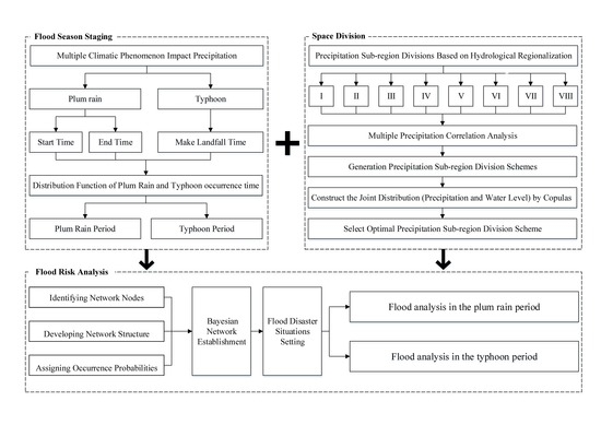
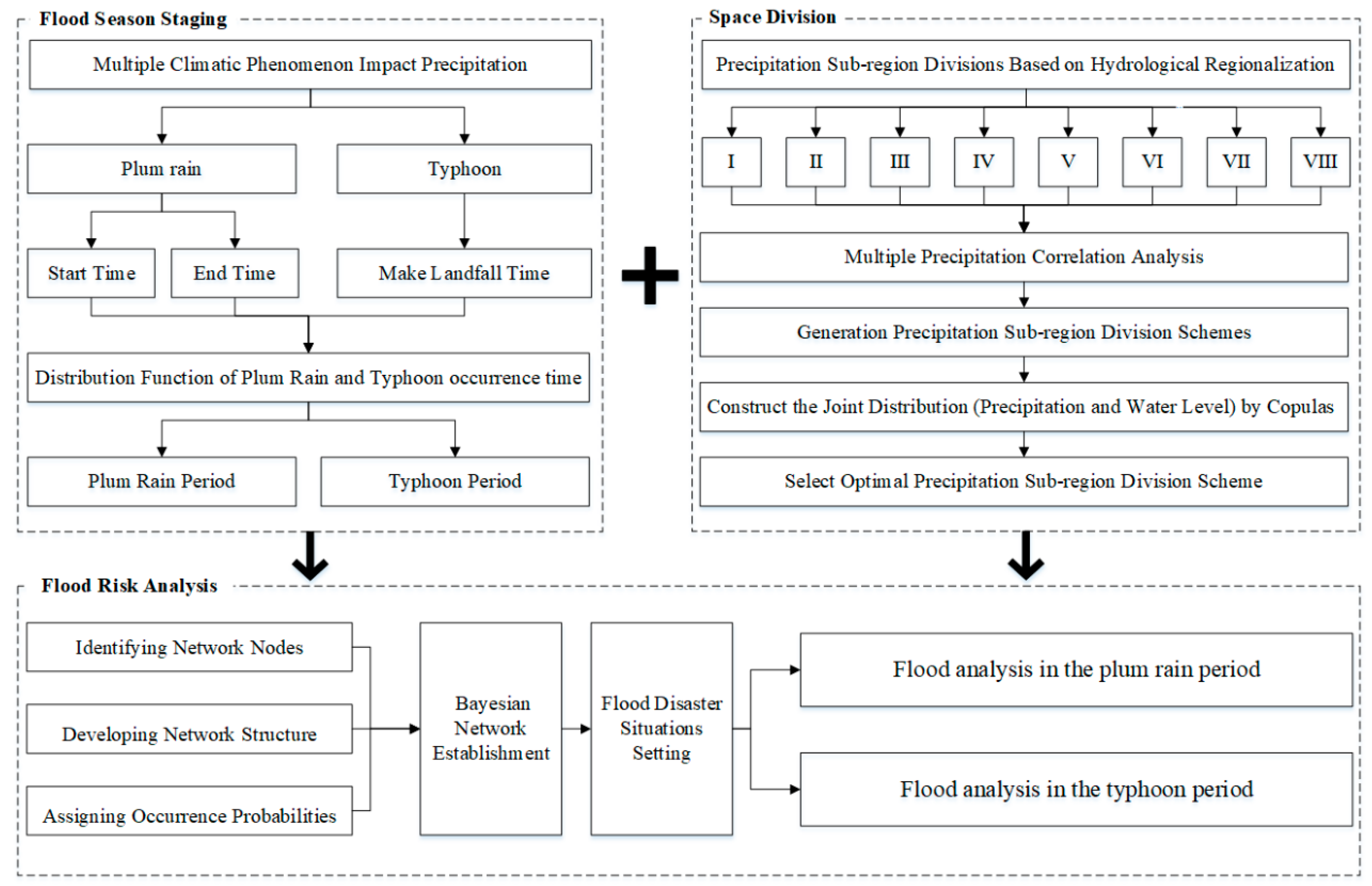
The framework of this study is shown in Figure 2. The programs of this paper such as copula functions were implemented in R programming language.

4. Results

4.1. Results of Flood Season Staging

Table 3. Parameters of six reference distributions.

	Param	Normal	Lognormal	Gamma	Weibull	Logistic	Beta
STP	Param#1	189.10	5.24	414.96	21.10	189.02	200.10
	Param#2	9.27	0.05	2.19	193.52	5.27	186.15
ETP	Param#1	165.50	5.11	407.16	22.62	166.03	227.00
	Param#2	8.09	0.05	2.46	169.15	4.39	273.66
ITT	Param#1	220.86	5.38	39.76	6.83	220.92	15.05
	Param#2	34.49	0.16	0.18	235.55	19.65	9.80

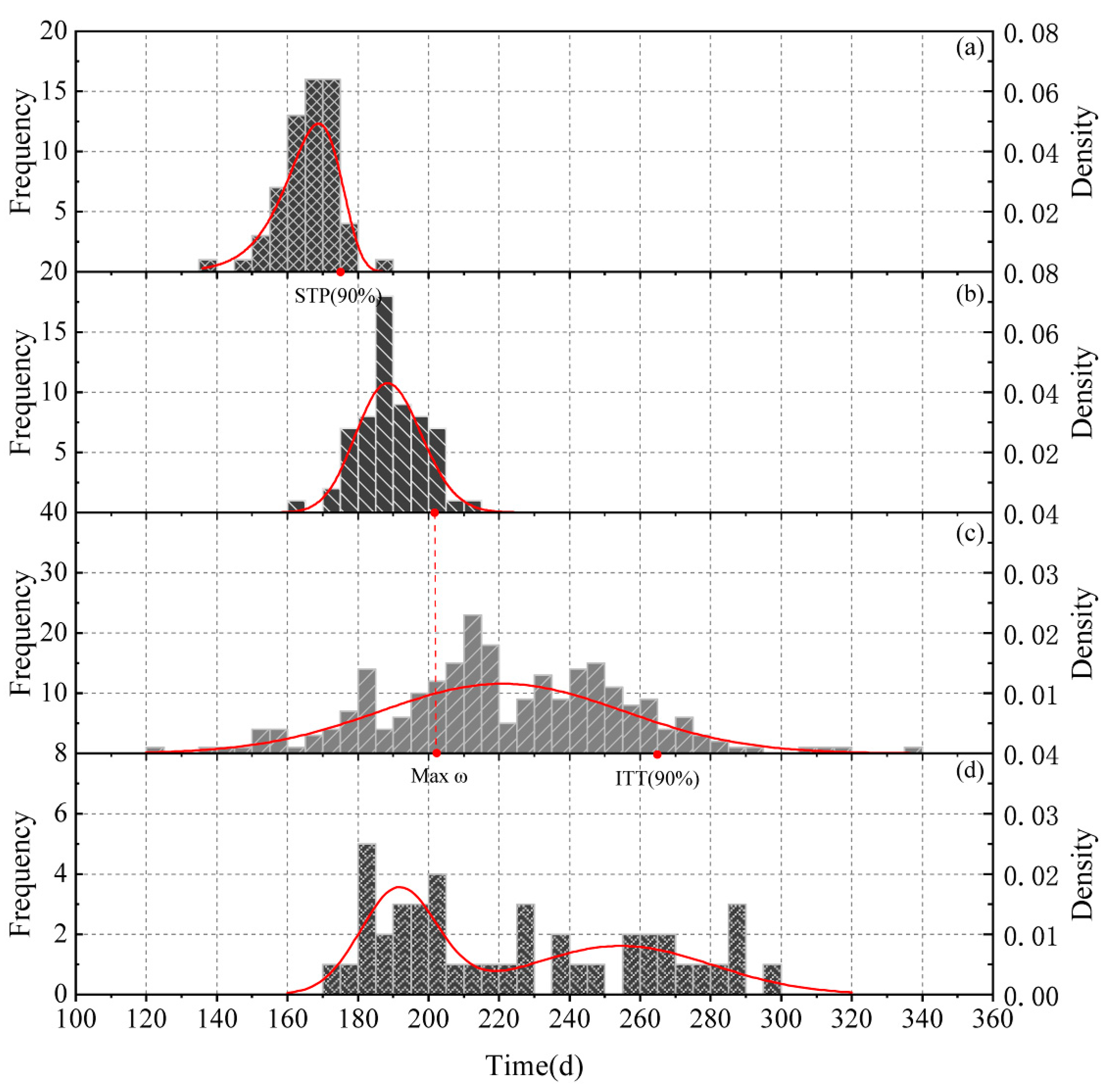
NOTES: Param#1 and Param#2 are the location and scale parameters of each distribution.

lists the parameters of six reference distributions. The results of the K-S test and other goodness-of-fit tests are shown in

Table 4. K-S test results of random variables with six reference distribution.

	Statistic	Normal	Lognormal	Gamma	Weibull	Logistic	Beta
STP	acceptance	accept	refuse	accept	accept	accept	refuse
	D	0.116	0.122	0.120	0.083	0.095	0.126
ETP	acceptance	accept	accept	accept	refuse	accept	accept
	D	0.079	0.070	0.071	0.120	0.074	0.080
ITT	acceptance	accept	accept	accept	refuse	accept	refuse
	D	0.050	0.056	0.051	0.075	0.053	0.064

, and

Table 5. Goodness-of-fit tests for start time of the plum rain period (STP), plum rain period (ETP), and initial time when typhoon begins to affect the Taihu Basin (ITT).

	Distribution	PPCC	MAE	RMSE	DC
STP	Normal	0.93806	0.07608	0.00664	0.99884
	Lognormal	0.86239	0.08376	0.00793	0.99834
	Gamma	0.87721	0.08127	0.0075	0.99852
	Weibull	0.98716	0.05248	0.00314	0.99974
	Logistic	0.92573	0.0717	0.00616	0.999
	Beta	0.89938	0.07707	0.0068	0.99878
ETP	Normal	0.97582	0.04382	0.00245	0.9998
	Lognormal	0.98705	0.0401	0.00201	0.99987
	Gamma	0.98544	0.04088	0.00212	0.99985
	Weibull	0.81086	0.08068	0.00728	0.99825
	Logistic	0.98186	0.05228	0.00358	0.99958
	Beta	0.97941	0.04404	0.00248	0.9998
ITT	Normal	0.97432	0.02271	0.00069	0.99995
	Lognormal	0.94455	0.0288	0.00105	0.99987
	Gamma	0.96392	0.02624	0.00064	0.99991
	Weibull	0.93664	0.03021	0.00109	0.99985
	Logistic	0.9652	0.02909	0.00112	0.99985
	Beta	0.97077	0.02275	0.00085	0.99994

, respectively. Figure 3 shows the probability density functions of STP, ETP, ITT, and TWL.

Table 4 and Table 5 show that the Weibull distribution, Log-normal distribution, and Normal distribution are the most suitable distribution functions for STP, ETP, and ITT, respectively (these results are similar to the previous study [33]). From Figure 2a–c, shows that the plum rain period is from June 24 (175th day, when the STP cumulative is 90%) to July 21 (202nd day, with the maximum ω value) and the typhoon period is from July 22 (203rd day) to September 22 (265th day, when the ITT cumulative is 90%).

Three conclusions can be drawn from Figure 3d, as follows: (1) during 170th to 180th days, the probability of the water level of Taihu Lake exceeding the warning water level increases rapidly, indicating that precipitation increases during this period. The June 24 (175th day) serving as the start time of the plum rain period is therefore rational; (2) on July 10 (191st day), the probability of the water level of the Taihu Lake exceeding the warning water level (3.8 m) is highest during the plum rain period. On August 4 (216th day), the probability of the actual water level of Taihu Lake exceeding the warning water level is lowest. This means that the demarcation point of the plum rain period and the typhoon period is after July 10 and before August 4. Therefore, July 21 (202nd day) is considered reasonably as the end of the plum rain period and start of typhoon period; (3) The shape of the PDF of TWL during the plum rain period (175th to 202nd day) is high and thin, whereas during the typhoon period (203rd to 265th day) it is low and fat. This phenomenon is consistent with the precipitation characteristics of the plum rain period and the typhoon period.

4.2. Results of Hydrological Sub-Region Clustering

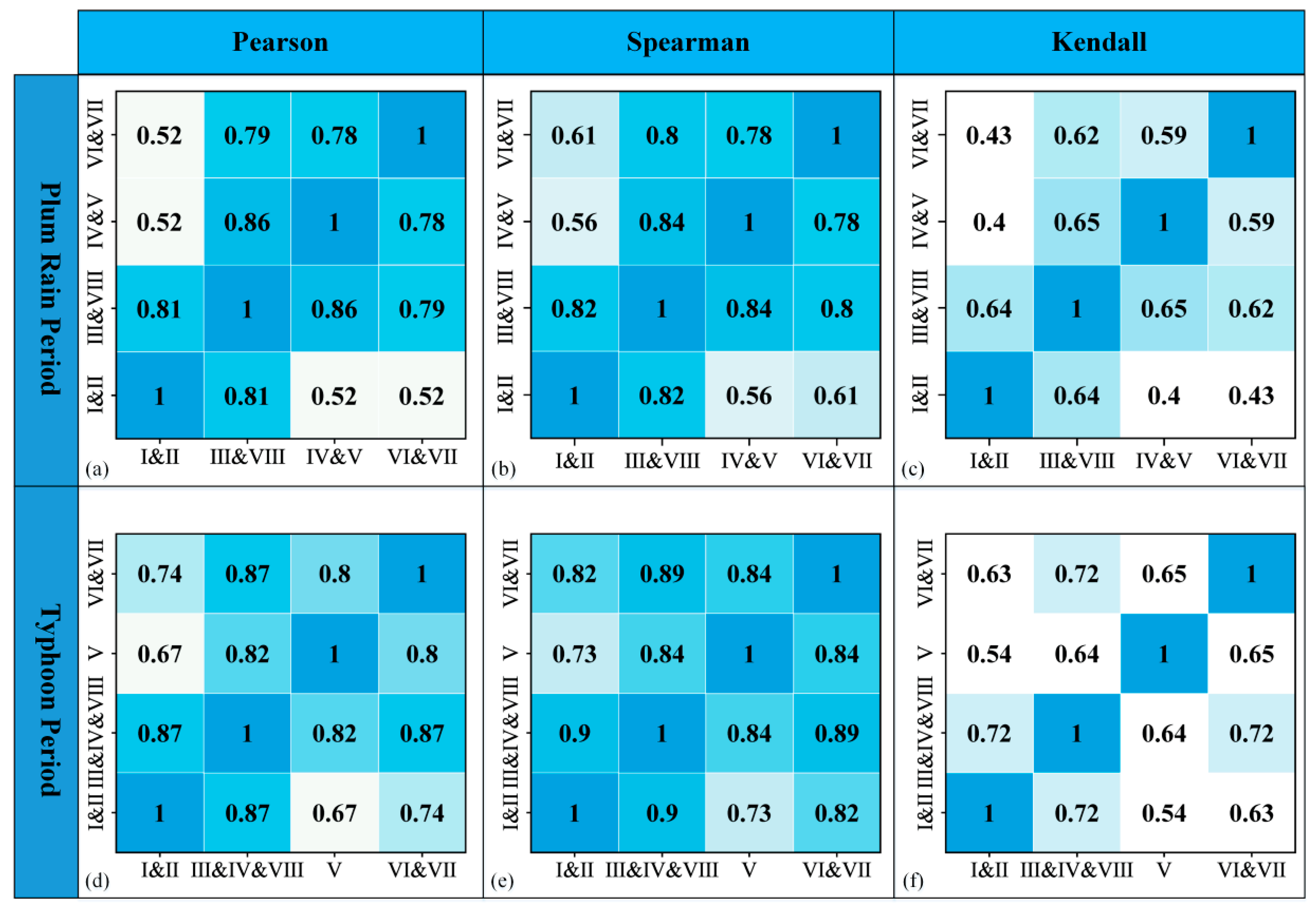
As shown in Figure 4a–c, as regards the geographic topological relation, for the plum rain period, the eight hydrological sub-regions were merged into four precipitation sub-regions (I and II, III and VIII, IV and V, VI and VII). As shown in Figure 4d–e, during the typhoon period, the eight hydrological sub-regions were merged into four precipitation sub-regions (I and II, III and VIII, IV and V, VI and VII).

Subsequently, the second division was implemented. As shown in Figure 5a–c, the figures show that the precipitation correlation between the III and VIII sub-region and IV and V sub-region is still high. Therefore, the III and VIII sub-region and IV and V sub-region were merged in the plum rain period. Figure 5d–f shows that the precipitation correlation between every pair of the four sub-regions is strong, indicating that the spatial heterogeneity of precipitation is not apparent in the typhoon period. However, to compare with the plum rain period, the second division of the typhoon period was kept consistent with that of the plum rain period.

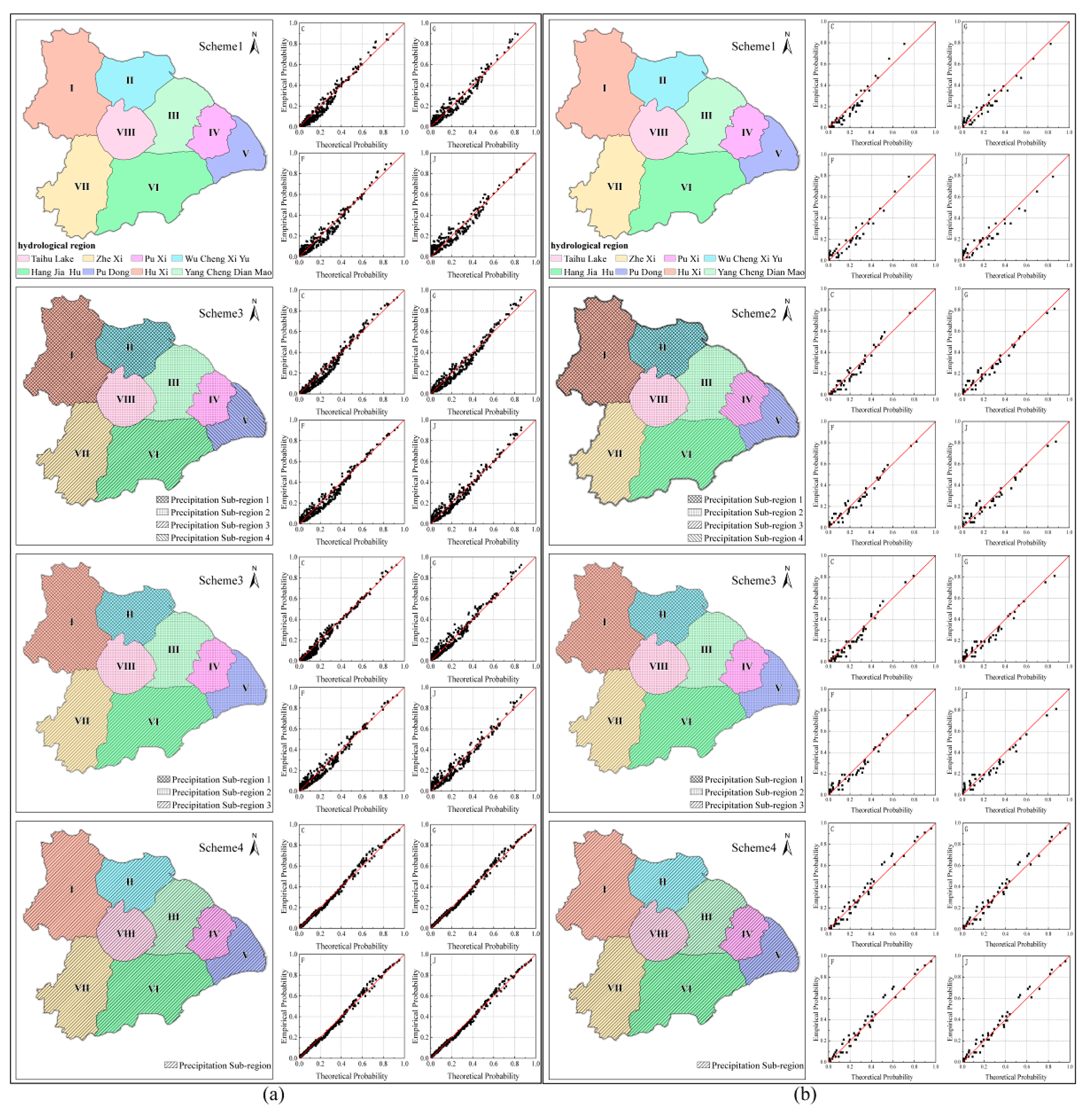
After two precipitation sub-region divisions, the four schemes were calculated for the plum rain period, and typhoon periods, respectively. The joint distribution of regional precipitation and the Taihu Lake water level were calculated by Archimedean copulas in each scheme. The results are shown in Figure 6.

As shown in

Table 6. Goodness-of-fit tests for the copula functions in the plum rain and typhoon periods.

Time	Copulas	AIC				BIC
		Scheme 1	Scheme 2	Scheme 3	Scheme 4	Scheme 1	Scheme 2	Scheme 3	Scheme 4
Plum rain period	Clayton	−181	−188	−189	−176	−175	−182	−183	−171
	Gumbel	−174	−180	−175	−178	−168	−174	−169	−173
	Frank	−164	−172	−173	−176	−158	−166	−167	−170
	Joe	−158	−167	−164	−181	−152	−161	−158	−175
Typhoo-n period	Clayton	−1124	−1197	−1193	−1775	−1113	−1185	−1181	−1763
	Gumbel	−1131	−1176	−1179	−1792	−1120	−1164	−1168	−1780
	Frank	−1045	−1123	−1133	−1753	−1033	−1112	−1121	−1741
	Joe	−989	−1062	−1080	−1803	−977	−1051	−1069	−1792

, in the plum rain period, the Clayton copula was selected to be the best-fitting copulas for Scheme 1, Scheme 2, and Scheme 3, whereas the Joe copula best fits the data in Scheme 4. In the typhoon period, the Gumbel copula was selected for Scheme 1, the Clayton copula for Scheme 2 and Scheme 3, And the Joe copula for Scheme 1.

Subsequently, the optimal divisions for plum rain period and typhoon period were selected according to the optimal copula of each scheme. Based on the minimum value criterion of AIC and BIC, it is clear that the Scheme 3 and Scheme 4 best describe the relation of the precipitation and the Taihu Lake water level during the plum rain period, and the typhoon period, respectively. Accordingly, the final results of precipitation sub-region division as follows: (1) in the plum rain period, the Taihu Basin is divided into P-I sub-region, P-II sub-region, and P-III sub-region; (2) in the typhoon period, the Taihu Basin as a whole for flood risk analysis (Figure 7).

4.3. Risk Management Model for Flood Control and Drainage in the Taihu Basin

4.3.1. The Result of Flood Disaster Situation Setting

The conducive and adverse drainage situations were designed according to the flood control planning of the Taihu Basin drawn up by the TBA.

In the plum rain period, when the water level of Taihu Lake exceeds the warning water level, it is unfavorable for flood drainage as long as a rainstorm with a return period over 50 years occurs in one of the four sub-regions. The 16 situations are shown in

Table 7. Calculation of encounter probability during the plum rain period.

Conducive Drainage Situation

P-I precipitation

Low

Low

Low

Low

High

Low

High

High

High

P-II precipitation

Low

Low

Low

High

Low

High

Low

High

High

P-III precipitation

Low

Low

High

Low

Low

High

High

Low

High

Taihu Lake water level

↑

↓

↓

↓

↓

↓

↓

↓

↓

Encounter probability

12.183

81.978

0.956

1.019

1.142

0.143

0.17

0.052

0.001

Adverse Drainage Situation

P-I precipitation

High

Low

Low

High

High

High

Low

P-II precipitation

High

Low

High

Low

High

Low

High

P-III precipitation

High

High

Low

Low

Low

High

High

Taihu Lake water level

↑

↑

↑

↑

↑

↑

↑

Encounter probability

0.021

0.878

0.411

0.171

0.58

0.157

0.137

NOTES: Low means precipitation with a return period of less than 50 years; High means precipitation with a return period of more than 50 years. The upwards, arrow and down arrow symbols mean the Taihu Lake water level is lower, or higher than the warning water level, respectively. The encounter probability is expressed as percentage.

.

In the typhoon period, it is unfavorable for flood drainage if a rainstorm occurs in the Taihu Basin with a return period of more than 100 years, and the water level of Taihu Lake exceeds the warning water level. Alternatively, it is unfavorable if a rainstorm occurs in the Taihu Basin with a return period between 50 and 100 years and simultaneously, the Taihu Lake water level exceeds the safety guarantee level. The nine situations are shown in

Table 8. Calculation of encounter probability during the typhoon period.

	Conducive Drainage Situation						Adverse Drainage Situation
Taihu Basin Precipitation	Low	Middle	Middle	Low	Low	High	High	Middle	High
Taihu Lake water level	↓	↔	↓	↔	↑	↓	↔	↑	↑
Encounter probability	86.52	0.74	8.44	2.25	1.21	0.04	0.01	0.75	0.05

NOTES: Low means precipitation with a return period of less than 50 years; middle means precipitation with a return period between 50 and 100 years. High means precipitation with a return period of more than 100 years. The downwards arrow symbol means the Taihu Lake water level is lower than the warning water level. The upwards arrow symbol means the Taihu Lake water level is higher than the water level with safety guarantee. The double arrow symbol means the Taihu Lake water level is between the warning water level and the water level with safety guarantee.

.

4.3.2. The Result of Copula-Based Bayesian Network Model

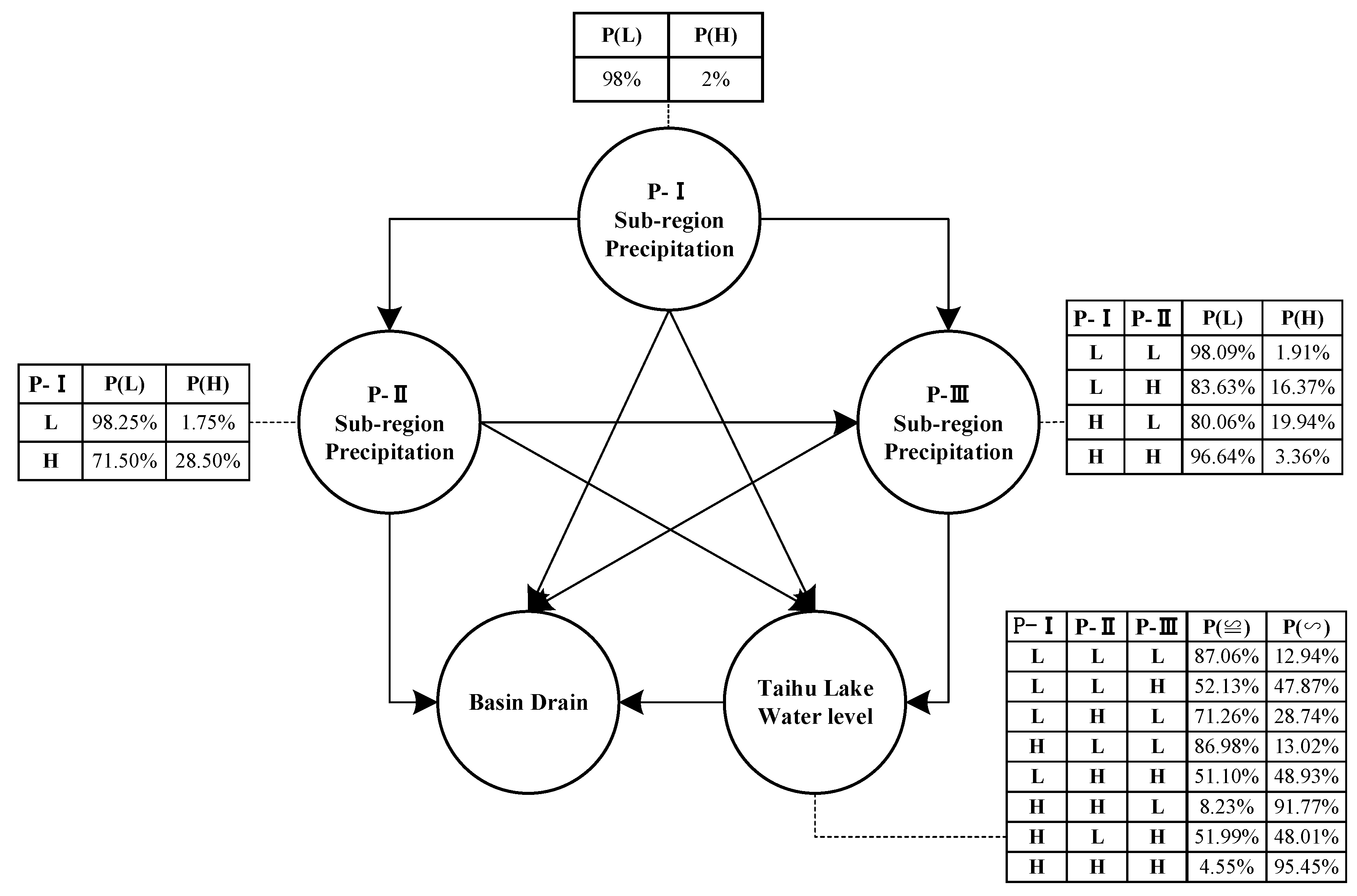
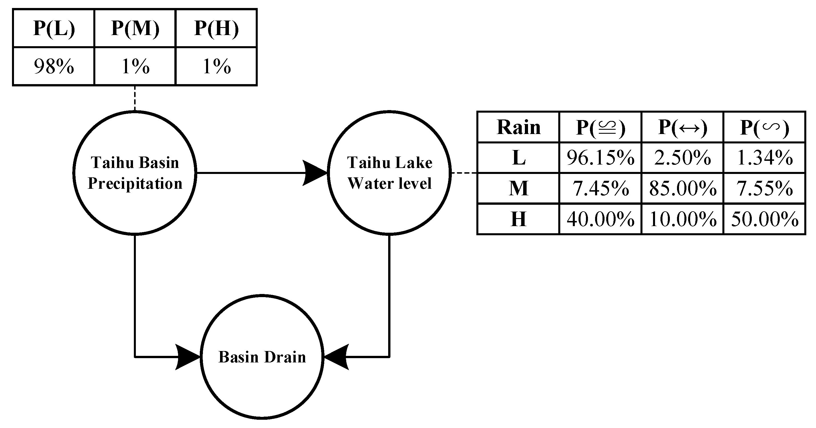
As shown in the Table 7 and Table 8, future total probabilities for adverse drainage situations in the Taihu Basin during the plum rain period and the typhoon period are 2.4%, and 0.8%, respectively. The Bayesian network structures of the flood risk management model during the plum rain period and the typhoon period are shown in Figure 8 and Figure 9. In the plum rain period, the Bayesian network structures of the flood risk management model has five network nodes (the circles in Figure 8). The P-I sub-region precipitation is a parent node and the Taihu Basin drainage situation is a child node, whereas the others are norm nodes. The directed edges between the network nodes represent correlations between variables, and the tables beside the network nodes are occurrence probabilities in different situations. In the typhoon period, the Bayesian network structures of the flood risk management model has three network nodes (the circles in Figure 9). The precipitation of the Taihu Basin is a parent node, the Taihu Basin drainage situation is a child node, and the Taihu Lake water level is a norm node. The means of the symbols in Figure 9 are the same as those of Figure 8.

5. Discussion

5.1. Rationality Analysis of the Precipitation Sub-Region Division Results

To determine whether the precipitation sub-region division results are reasonable, we analyzed the amount and structure of precipitation in the Taihu Basin during the different periods.

The precipitation concentration degree (PCD) and the precipitation concentration period (PCP) are new parameters characterizing the precipitation structure [49], calculated as follows:

$$\begin{gathered} PC{D}_i=\sqrt{R_{xi}^2+R_{yi}^2}/R_i \\ PC{P}_i=\arctan (R_{xi}/R_{yi}) \\ {R}_{xi}={\displaystyle \sum _{j=1}^N{r}_{ij}\sin {\theta }_j};R_{yi}={\displaystyle \sum _{j=1}^N{r}_{ij}\cos {\theta }_j} \end{gathered}$$

(11)

where PCD_i, and PCP_i, respectively, are the precipitation concentration degree and concentration period in the research time; R_i is the total precipitation in the research time, and r_ij is the precipitation in five days. θ_j is the corresponding azimuth angle in the research time (the entire research time is 360°); i is the year (i = 1954, … ,2011); j is a five day series in the research time.

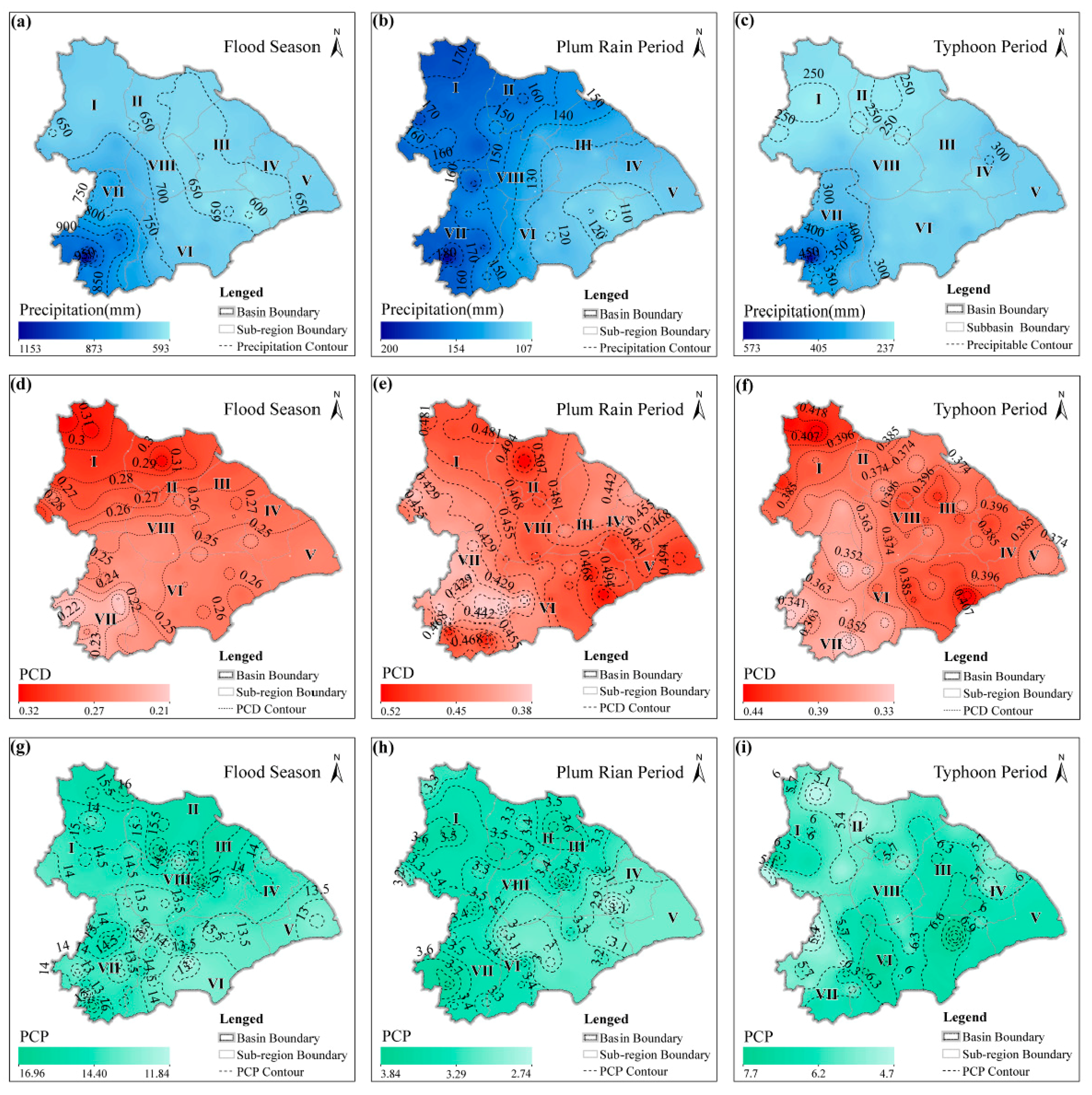
We drafted isograms (precipitation amount, PCD, PCP), which are useful in demonstrating the spatial and temporal heterogeneity of precipitation.

According to Figure 10a, in the flood season, more precipitation occurs over the west and the south of the basin, and the rainfall over the south is higher than over the north. There are three precipitation grades from the southwest to the northeast. However, it is vastly different in the plum rain period. As shown in Figure 10b, there are two maximum precipitation regions in the northwest and southwest of the Taihu Basin. Figure 10c shows that the spatial distribution of precipitation is homogeneous, except for the VII sub-region in the typhoon period. Figure 10d–f shows that the PCD values and spatial distribution differ during the different periods. In the flood season, the PCD value shows a decreasing trend from northwest to southeast. However, the distribution of the PCD maximum regions is dispersive in the plum rain period and typhoon period. Figure 10h–j shows that the average PCP of the plum rain period, the typhoon period, and the flood season appear in the 3rd pentad (early July), the 6th pentad (late August) and the 15th pentad (middle July), respectively. In conclusion, if the whole flood season was selected to study the heterogeneity of precipitation, the precipitation characteristics of the different climatic phenomena would not be revealed.

The water level of the Taihu Lake plays a significant role in flood control. The amount of precipitation is the reason for the Taihu Lake water level. According to the Figure 7a and Figure 10b, the result of precipitation sub-region division in the plum rain period corresponds to the spatial distribution of precipitation amount. Similarly, the result of precipitation sub-region division in the typhoon period corresponds to the spatial distribution of precipitation amount, as shown in Figure 10c and Figure 7b.

5.2. Risk Analysis of Flood Disaster in the Taihu Basin During Different Periods

5.2.1. Flood Analysis in the Plum Rain Period

Based on a posterior knowledge input, the backward reasoning function of the Bayesian network was used to conduct simulation calculations of the Taihu Lake water level states in some certain precipitation situations that could occur in the plum rain period [50,51]. These precipitation situations are shown in

Table 9. Situation-setting of precipitation in the plum rain period.

Situation	P-I Precipitation	P-II Precipitation	P-III Precipitation	Taihu Lake Water Level
A	Is High	High or Low?	High or Low?	↑or↓?
B	Is High	Is High	High or Low?	↑or↓?
C	Is High	Is High	Is High	↑or↓?

NOTES: The definitions of “Low”, “High” “↑” and “↓” are the same as for Table 7.

.

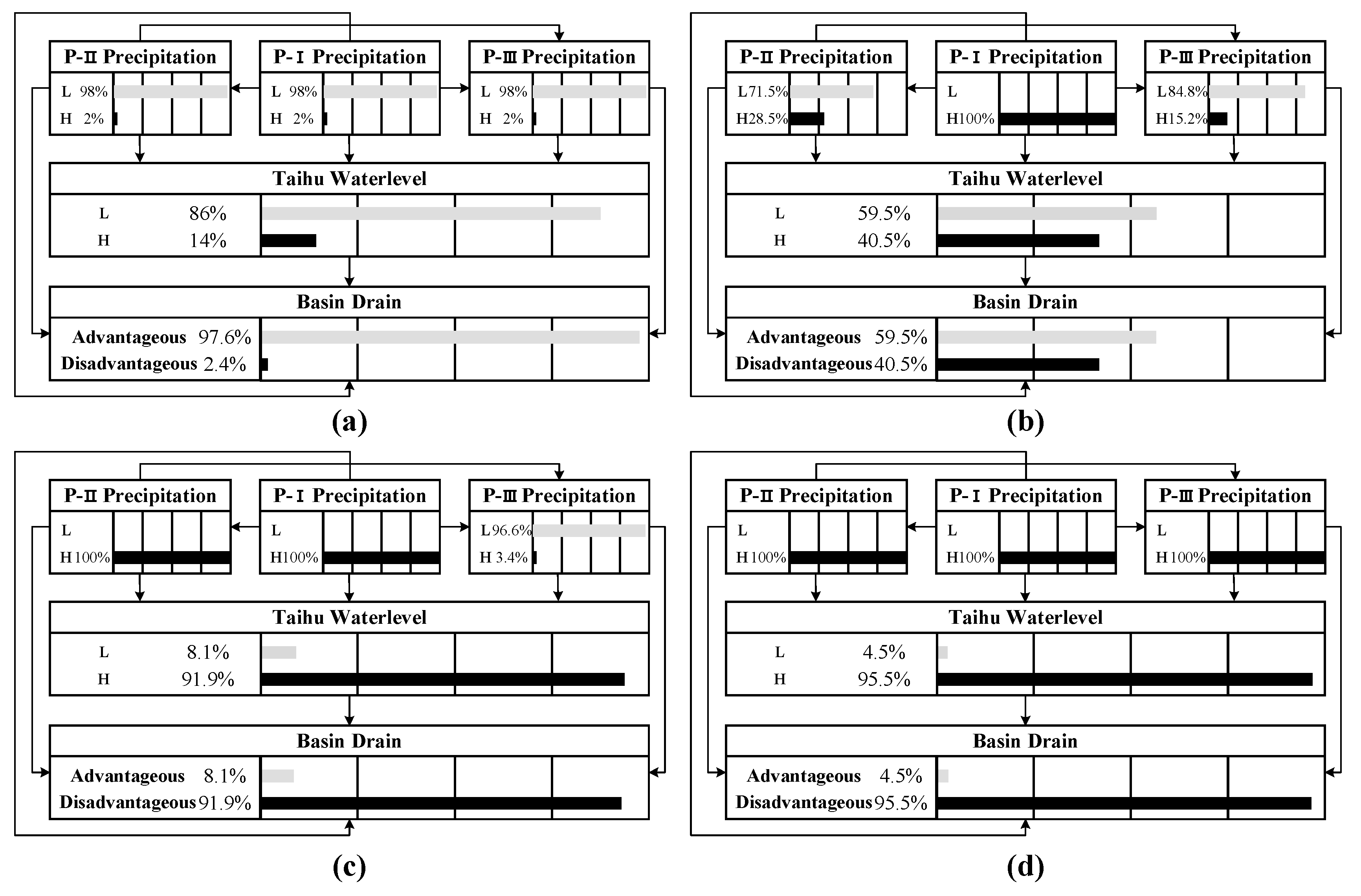
According to Figure 11a,b, the probability of the Taihu Lake water level rising beyond 3.8 m increases dramatically when the P-I precipitation sub-region encounters a rainstorm with a return period of more than 50 years, which in turn, increases the risk of flood disaster up to 40.5%. According to Figure 11b,c, the probability of the Taihu Lake water level exceeding 3.8 m increases again when the P-I precipitation sub-region and P-II precipitation sub-region encounter a rainstorm with a return period of more than 50 years at the same time. In such instances, the risk of flood disaster in the Taihu Basin increases to 91.9%. According to Figure 11c,d, when all precipitation sub-regions encounter the rainstorm with a return period over 50 years simultaneously, the probability of flood disaster increases from 91.9% to 95.5%.

In the plum rain period, the P-I precipitation sub-region and P-II precipitation sub-region are considered maximum precipitation regions. These precipitation sub-regions in the upper reaches of the Taihu Basin are hilly areas, with fast water flow and a short flow concentration time. Furthermore, the runoff of P-I precipitation sub-region and P-II precipitation sub-region mostly flows into the Taihu Lake. However, the P-III precipitation sub-region is located in the lower reaches of the Taihu Basin, which are plain areas with slow water flow. Accordingly, more attention should be paid to the precipitation of P-I precipitation sub-region and P-II precipitation sub-region during the plum rain period. However, the precipitation of P-III precipitation sub-region should be monitored continuously, as it could cause poor drainage in the lower reaches.

5.2.2. Flood Analysis in the Typhoon Period

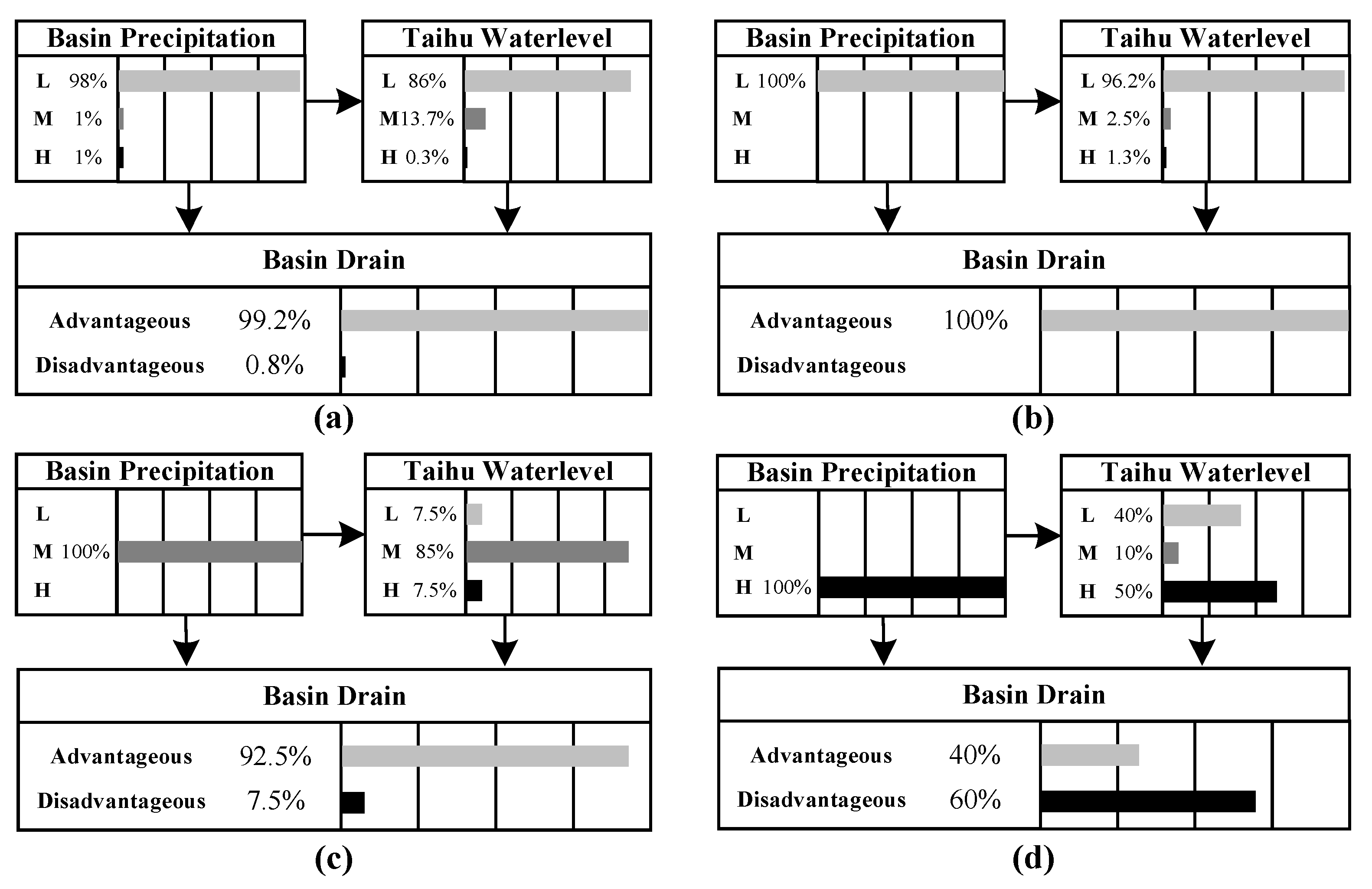
The precipitation situations of the typhoon period are as

Table 10. Situation-setting of precipitation in the typhoon period.

Situation	Taihu Basin Precipitation	Taihu Lake Water Level
A	Is Low	↑ or ↔ or ↓?
B	Is Middle	↑ or ↔ or ↓?
C	Is High	↑ or ↔ or ↓?

NOTES: The definitions of “Low”, “Middle”, “High”, “↑”, “↔” and “↓” are the same as Table 8.

shown. According to Figure 12a,b, when the Taihu Basin encounters a rainstorm with a return period of less than 50 years, there is little likelihood of a flood disaster. However, as shown in Figure 12b,c, when the Taihu Basin encounters a rainstorm with a return period between 50 years and 100 years, the probability of the Taihu Lake water level being 3.8 m to 4.65 m is up to 85%. This increases the risk of flood disaster slightly. According to Figure 12c,d, when the Taihu Basin encounters a rainstorm with a return period of more than 100 years, the probability of the Taihu Lake water level rising above 4.65 m increases dramatically and the probability of flood disaster in the Taihu Basin increases from 7.5% to 60%.

In the typhoon period, the spatial heterogeneity of precipitation is not obvious. Therefore, we focused on precipitation over the entire basin. In particular, rainstorms with a return period of more than 100 years should generally be monitored.

6. Conclusions

To analyze the flood disaster risk in the Taihu Basin, we divided the flood season into the plum rain period and the typhoon period, due to different precipitation heterogeneous in different climatic phenomena. Subsequently, we divided the Taihu Basin into precipitation sub-regions by using Copula functions. Finally, based on Bayesian network theory, we proposed a risk management model for flood control in the Taihu Basin to analyze the flood disaster during the different periods. The main conclusions of this study are as follows:

• Due to meteorological reasons, the occurrence time of plum rain and typhoon present regularity, resulting in uneven distribution of precipitation during the flood season. Our flood season staging indicated that the plum rain period is from June 24 to July 21 and the typhoon period is from July 22 to September 22.
• The spatial heterogeneity of precipitation is different under the influence of the different climatic phenomena. In the plum rain period, the Taihu Basin is divided into three precipitation sub-regions (P-I, P-II, and P-III). In the typhoon period, the Taihu Basin serves as a whole for flood risk analysis.
• In future, the occurrence probability of adverse drainage situations in the Taihu Basin during the plum rain period and the typhoon period is 2.4%, and 0.8%, respectively. Furthermore, the risk increases rapidly as the Taihu Lake water level rises.
• Although the annual precipitation of the Taihu Basin is concentrated in the flood season, the precipitation heterogeneous varies with the differing climatic phenomena. This implies that the risks of flood disaster also differs. Consequently, appropriate emergency plans should be developed to prevent and manage flood disasters occurring in the different periods during the flood season.

In this study, the Taihu Basin was used as a case study to analyze the flood risk of different climatic phenomena. Further research, employing the proposed methodology of our study, could be conducted in the coastal areas of East Asia, such as Taiwan, the Liaodong Peninsula, and Japan that are also affected by typhoons and plum rains. Given the considerable risk of flooding in the coastal areas of East Asia, it is crucial that flood season staging scheduling for flood control be implemented.

References

1. Favre, A.-C.; El Adlouni, S.; Perreault, L.; Thiémonge, N.; Bobée, B. Multivariate hydrological frequency analysis using copulas. Water Resour. Res. 2004, 40. [Google Scholar] [CrossRef] [Green Version]
2. Karmakar, S.; Simonovic, S. Bivariate flood frequency analysis. Part 2: A copula-based approach with mixed marginal distributions. J. Flood Risk Manag. 2009, 2, 32–44. [Google Scholar]
3. Mouri, G.; Minoshima, D.; Golosov, V.; Chalov, S.; Seto, S.; Yoshimura, K.; Nakamura, S.; Oki, T. Probability assessment of flood and sediment disasters in japan using the total runoff-integrating pathways model. Int. J. Disaster Risk Reduct. 2013, 3, 31–43. [Google Scholar]
4. Pandey, A.C.; Singh, S.K.; Nathawat, M.S. Waterlogging and flood hazards vulnerability and risk assessment in indo gangetic plain. Nat. Hazards 2010, 55, 273–289. [Google Scholar]
5. Romanescu, G.; Hapciuc, O.; Minea, I.; Iosub, M. Flood vulnerability assessment in the mountain–plateau transition zone: A case study of marginea village (Romania). J. Flood Risk Manag. 2018, 11, S502–S513. [Google Scholar]
6. Jamshed, A.; Rana, I.A.; Mirza, U.M.; Birkmann, J. Assessing relationship between vulnerability and capacity: An empirical study on rural flooding in Pakistan. Int. J. Disaster Risk Reduct. 2019, 36, 101109. [Google Scholar]
7. Smith, D.I. Flood damage estimation-a review of urban stage-damage curves and loss functions. Water Sa 1994, 20, 231–238. [Google Scholar]
8. Feng, P.; Cui, G.-T.; Zhong, Y. On the evaluation and prediction of urban flood economic loss. J. Hydraul Eng. 2001, 8, 64–68. [Google Scholar]
9. Jonkman, S.N.; Bočkarjova, M.; Kok, M.; Bernardini, P. Integrated hydrodynamic and economic modelling of flood damage in The Netherlands. Ecol. Econ. 2008, 66, 77–90. [Google Scholar]
10. Bonasia, R.; Areu-Rangel, O.; Tolentino, D.; Mendoza-Sanchez, I.; González-Cao, J.; Klapp, J. Flooding hazard assessment at Tulancingo (Hidalgo, Mexico). J. Flood Risk Manag. 2018, 11, S1116–S1124. [Google Scholar]
11. Fakhruddin, S.H.M.; Kawasaki, A.; Babel, M.S. Community responses to flood early warning system: Case study in Kaijuri Union, Bangladesh. Int. J. Disaster Risk Reduct. 2015, 14, 323–331. [Google Scholar]
12. Zaw, T.N.; Lim, S. The military’s role in disaster management and response during the 2015 myanmar floods: A social network approach. Int. J. Disaster Risk Reduct. 2017, 25, 1–21. [Google Scholar]
13. McCallum, I.; Liu, W.; See, L.; Mechler, R.; Keating, A.; Hochrainer-Stigler, S.; Mochizuki, J.; Fritz, S.; Dugar, S.; Arestegui, M. Technologies to support community flood disaster risk reduction. Int. J. Disaster Risk Sci. 2016, 7, 198–204. [Google Scholar]
14. Jiang, X.; Yang, L.; Tatano, H. Assessing spatial flood risk from multiple flood sources in a small river basin: A method based on multivariate design rainfall. Water 2019, 11, 1031. [Google Scholar]
15. Zhou, T.; Liu, Z.; Jin, J.; Hu, H. Assessing the impacts of univariate and bivariate flood frequency approaches to flood risk accounting for reservoir operation. Water 2019, 11, 475. [Google Scholar]
16. Xie, H.; Huang, J.S. A review of bivariate hydrological frequency distribution. Adv. Water Sci. 2008, 19, 443–452. [Google Scholar]
17. Bacchi, B.; Becciu, G.; Kottegoda, N.T. Bivariate exponential model applied to intensities and durations of extreme rainfall. J. Hydrol. 1994, 155, 225–236. [Google Scholar]
18. Goel, N.; Seth, S.; Chandra, S. Multivariate modeling of flood flows. J. Hydraul. Eng. 1998, 124, 146–155. [Google Scholar]
19. Yue, S. The gumbel logistic model for representing a multivariate storm event. Adv. Water Resour. 2001, 24, 179–185. [Google Scholar]
20. Long, D.; Krzysztofowicz, R. Farlie-gumbel-morgenstern bivariate densities: Are they applicable in hydrology? Stoch. Hydrol. Hydraul. 1992, 6, 47–54. [Google Scholar]
21. Kelly, K.S.; Krzysztofowicz, R. A bivariate meta-gaussian density for use in hydrology. Stoch. Hydrol. Hydraul. 1997, 11, 17–31. [Google Scholar]
22. Salvadori, G.; De Michele, C. Frequency analysis via copulas: Theoretical aspects and applications to hydrological events. Water Resour. Res. 2004, 40. [Google Scholar] [CrossRef]
23. Fang, B.; Guo, S.L.; Xiao, Y.; Liu, P.; Jian, W.U. Annual maximum flood occurrence dates and magnitudes frequency analysis based on bivariate joint distribution. Adv. Water Sci. 2008, 19, 505–511. [Google Scholar]
24. Lian, J.J.; Xu, K.; Ma, C. Joint impact of rainfall and tidal level on flood risk in a coastal city with a complex river network: A case study of Fuzhou city, China. Hydrol. Earth Syst. Sci. 2013, 17, 679–689. [Google Scholar]
25. Ai, P.; Yuan, D.; Xiong, C. Copula-based joint probability analysis of compound floods from rainstorm and typhoon surge: A case study of Jiangsu coastal areas, China. Sustainability 2018, 10, 2232. [Google Scholar]
26. Wang, W.; Dong, Z.; Si, W.; Zhang, Y.; Xu, W. Two-dimension monthly river flow simulation using hierarchical network-copula conditional models. Water Resour. Manag. 2018, 32, 3801–3820. [Google Scholar]
27. Shiau, J.T.; Wang, H.Y.; Tsai, C.T. Bivariate frequency analysis of floods using copulas. JAWRA J. Am. Water Resour. Assoc. 2010, 42, 1549–1564. [Google Scholar]
28. Liu, Y.; Wang, Y.; Hu, Q.; Cui, T.; Wang, L. Characteristics analysis of plum rains in taihu lake basin based on joint distribution. Hydro-Sci. Eng. 2015, 4, 98–105. [Google Scholar]
29. Liu, Z.M.; Chen, Z.S. Risk study of the bivariate encounter of interzone rainstorm and flood level of the outer river. Adv. Water Sci. 2009, 20, 619–625. [Google Scholar]
30. Parker, K.; Hill, D.F. Evaluation of bias correction methods for wave modeling output. Ocean Model. 2017, 110, 52–65. [Google Scholar]
31. Yin, J.; Guo, S.; He, S.; Guo, J.; Hong, X.; Liu, Z. A copula-based analysis of projected climate changes to bivariate flood quantiles. J. Hydrol. 2018, 566, 23–42. [Google Scholar]
32. Lazoglou, G.; Anagnostopoulou, C.; Skoulikaris, C.; Tolika, K. Bias correction of climate model’s precipitation using the copula method and its application in river basin simulation. Water 2019, 11, 600. [Google Scholar]
33. Hu, S.; Wang, Z.; Wang, Y.; Wu, H.; Jin, J.; Feng, X.; Cheng, L. Encounter probability analysis of typhoon and plum rain in the taihu lake basin. Sci. China Technol. Sci. 2010, 53, 3331–3340. [Google Scholar]
34. Cui, T.; Wang, Y.; Liu, Y.; Wang, Z. Analysis of change trend of typhoon impacting taihu lake basin. J. China Hydrol. 2012, 32, 54–58. [Google Scholar]
35. Chebana, F.; Ouarda, T.B.M.J. Multivariate quantiles in hydrological frequency analysis. Environmetrics 2011, 22, 63–78. [Google Scholar] [Green Version]
36. Deng, P.X.; Hu, Q.-F.; Wang, Y.T.; Wang, L.Z.; Cui, T.T. Heterogeneity study of rainfall in the taihu lake basin. Hydro-Sci. Eng. 2014, 5, 34–40. [Google Scholar]
37. Taihu Basin Authority of Ministry of Water Resources. Taihu Basin Flood Control Planning; Taihu Basin Authority of Ministry of Water Resources: Shanghai, China, 2007. [Google Scholar]
38. Sklar, M. Fonctions de repartition an dimensions et leurs marges. Publ. Inst. Stat. Univ. Paris 1959, 8, 229–231. [Google Scholar]
39. Nelsen, R.B. An Introduction to Copulas; Springer Science & Business Media: New York, NY, USA, 2007. [Google Scholar]
40. Hofert, M.; Mächler, M.; McNeil, A.J. Likelihood inference for archimedean copulas in high dimensions under known margins. J. Multivar. Anal. 2012, 110, 133–150. [Google Scholar]
41. Omelka, M.; Veraverbeke, N.; Gijbels, I. Bootstrapping the conditional copula. J. Stat. Plan. Inference 2013, 143, 1–23. [Google Scholar]
42. Genest, C.; Rémillard, B.; Beaudoin, D. Goodness-of-fit tests for copulas: A review and a power study. Insur. Math. Econ. 2009, 44, 199–213. [Google Scholar]
43. Madadgar, S.; Moradkhani, H. A bayesian framework for probabilistic seasonal drought forecasting. J. Hydrometeorol. 2013, 14, 1685–1705. [Google Scholar]
44. Van de Vyver, H. Bayesian estimation of rainfall intensity-duration-frequency relationships. J. Hydrol. 2015, 529, 1451–1463. [Google Scholar]
45. Niedermayer, D. An introduction to bayesian networks and their contemporary applications. In Innovations in Bayesian Networks; Springer: Berlin/Heidelberg, Germany, 2008; pp. 117–130. [Google Scholar]
46. Kong, X.; Zeng, X.; Chen, C.; Fan, Y.; Huang, G.; Li, Y.; Wang, C. Development of a maximum entropy-archimedean copula-based bayesian network method for streamflow frequency analysis—A case study of the kaidu river basin, china. Water 2018, 11, 42. [Google Scholar]
47. Hanea, A.M.; Kurowicka, D.; Cooke, R.M. Hybrid method for quantifying and analyzing bayesian belief nets. Qual. Reliab. Eng. Int. 2006, 22, 709–729. [Google Scholar]
48. Hanea, A.; Napoles, O.M.; Ababei, D. Non-parametric bayesian networks: Improving theory and reviewing applications. Reliab. Eng. Syst. Saf. 2015, 144, 265–284. [Google Scholar]
49. Lujun, Z.; Yongfu, Q. Annual distribution features of precipitation in china and their interannual variations. J. Meteorol. Res. 2003, 17, 146–163. [Google Scholar]
50. He, X. Risk analysis of synchronous-asynchronous encounter probability of rich-poor precipitation in the middle route of south-to-north water. Adv. Water Sci. 2011, 22, 44–50. [Google Scholar]
51. Kang, L.; He, X.; Xiong, Q. Risk analysis for precipitation rich-poor encounter between source area and receiving area of the middle route of south-to-north water transfer project based on bayes-net theory. J. Hydraul. Eng. 2010, 41, 908–913. [Google Scholar]
Figure 1. Location of the study areas.
Water 11 01534 g001
Figure 2. Framework of flood risk analysis of the different climatic phenomena.
Water 11 01534 g002
Figure 3. Probability density functions of random variables. (a) start time of the plum rain period (STP); (b) plum rain period (ETP); (c) initial time when typhoon begins to affect the Taihu Basin (ITT); (d) Taihu Lake exceeds the warning water level (TWL).
Water 11 01534 g003
Figure 4. Correlation results of precipitation between eight hydrological regions. (ac) are the results for the plum rain period. (df) are the results for the typhoon period; (a,d) are Pearson correlation results; (b,e) are Spearman correlation results; (c,f) are Kendall correlation results.
Water 11 01534 g004
Figure 5. Correlation results of precipitation between four precipitation sub-regions. (ac) are the results for the plum rain period; (df) are the results for the typhoon period; (a,d) are Pearson correlation results; (b,e) are Spearman correlation results; (c,f) are Kendall correlation results.
Water 11 01534 g005
Figure 6. Precipitation sub-region divisions and the probability-probability plots of regional precipitation and the Taihu Lake water level in the typhoon period (a) and plum rain period (b). C is short for Clayton copula; G is short for Gumbel copula; F is short for Frank copula; J is short for Joe copula.
Water 11 01534 g006
Figure 7. Results of precipitation sub-region division in the plum rain period (a) and typhoon period (b).
Water 11 01534 g007
Figure 8. Bayesian network structure parameter map of the plum rain period.
Water 11 01534 g008
Figure 9. Bayesian network structure parameter map of the typhoon period.
Water 11 01534 g009
Figure 10. Isogram of precipitation amount (ac), precipitation concentration degree (PCD) (df), and precipitation concentration period (PCP) (gi) in the Taihu Basin.
Water 11 01534 g010
Figure 11. The priori reasoning of Bayesian network (a), and the posterior probability of various precipitation situations (bd) in the plum rain period.
Water 11 01534 g011
Figure 12. Priori reasoning of the Bayesian network (a), and the posterior probability of various precipitation situations (b), (c), (d) in the typhoon period.
Water 11 01534 g012