Article

Links between Teleconnection Patterns and Water Level Regime of Selected Polish Lakes

Institute of Physical Geography and Environmental Planning, Adam Mickiewicz University, Krygowskiego 10, 61-680 Poznań, Poland
*
Author to whom correspondence should be addressed.
Water 2019, 11(7), 1330; https://doi.org/10.3390/w11071330
Submission received: 30 May 2019 / Revised: 25 June 2019 / Accepted: 25 June 2019 / Published: 27 June 2019
(This article belongs to the Special Issue Effects of Oceanic-Atmospheric Oscillations on Rivers)

Abstract

:
The paper identifies relationships between lake water levels and indices of macroscale atmospheric circulations: Arctic Oscillation (AO), North Atlantic Oscillation (NAO), East Atlantic (EA), and Scandinavian pattern (SCAND). Correlation coefficients between synchronous and asynchronous series of monthly water levels and 4 circulation indices were calculated. Based on Ward hierarchical grouping considering 156 correlation coefficients, the groups of lakes were designated due to the strength and term of relation of circulation indices with lake water levels. It was found that these links are not strong but noticeable. The strength of relationships varies in space and time, and the designated groups of lakes refer not only to the climatic diversity of the studied area, but also to some extent to the types of water levels regime. The observed relationships are the most important in the case of AO and NAO (particularly in winter period), and slightly weaker for EA and SCAND. The analysis used mean monthly water levels of 15 lakes in northern Poland from 1976–2015.

1. Introduction

Water-level fluctuations are one of the basic characteristics of the hydrological regime of lakes determining the occurrence and course of many processes and phenomena affecting the functioning of a given water body [1]. Water level fluctuations are particularly determined by climatic factors and depth of the lake basin, connection with groundwaters, surface area and shape of the lake’s catchment, surface area of the lake itself, degree and character of its flow-through character, and human pressure. Climatic factors determining the volume of river and lake alimentation include atmospheric precipitation and air temperature. They are in turn to various degrees determined by teleconnection patterns. Climatic conditions in Europe show the most thoroughly documented effect of the Arctic Oscillation (AO) (e.g., on terms of snowmelts [2], ice cover of the Baltic Sea [3], variability of air temperatures in winter [4]), and North Atlantic Oscillation (NAO) (e.g., on maximum and minimum air temperatures, cloudiness, and precipitation [5], humid and warm winters, as well as among others the period of plant flowering [6], atmospheric precipitation, flow rates in rivers, and water resources [7]). The importance of the East Atlantic (EA) and Scandinavian patterns (SCAND) is investigated more seldom. The effect of EA on e.g., exceptionally low temperatures in winter 2010 [8] and temperatures in Serbia [9], as well as effect of SCAND and other teleconnection patterns on extreme precipitation [10] and thickness of snow cover [11] has been confirmed. The combined effect of different teleconnection patterns and relationships between them have also been analyzed [12]. AO is related to the difference in pressures between the polar area and moderate latitudes [13]. NAO is strongly associated with it, with activity depending on the difference between the Iceland Low and Azores High [14]. Also, EA concerns baric differences in the Atlantic region, although in the latitudinal system. SCAND concerns circulation related to North Europe and the surrounding baric centers [15]. Their activity affects the properties of climate in Poland, particularly NAO, as confirmed by available studies, among others in the context of occurrence of frosty days [16], duration of the vegetation period [17], air and lake water temperature [18], and occurrence of snow cover [19,20]. Wibig [15] investigated the influence of circulation patterns on precipitation in Europe in winter months. According to Central and East Europe region, the greatest impacts have SCAND and CE (Central Europe) patterns—the positive phase of SCAND brings very dry weather in eastern Europe, and in negative phase it favors precipitation. The influence of circulation patterns on air and water of lakes temperature in northern Poland was described by [18]. The strongest positive impact of NAO was observed from December to March, especially high in the western part of the area. The impact of AO was quite similar in winter, but it has also positive correlation with temperatures in September and October. EA has the strongest positive impact on thermal conditions from September to November. From January to March there were negative correlations of SCAND indices and air and water temperatures, and positive ones in May (only with air temperatures).
The authors point to temporal and spatial variability of the impact of particular circulation types at the scale of Poland on the analyzed hydrometeorological elements. In limnological literature concerning the importance of teleconnection patterns among others on hydrological variables, relatively few papers refer to water level regime of Polish lakes. Many papers ascribe particular importance to NAO, the effect of which on the thermal and ice regime is thoroughly investigated [18,21,22,23,24,25]. The importance of changes in the intensity of NAO for the water levels, their fluctuations, stability, and change tendencies is shown in research by, e.g., [1,26,27,28,29,30]. The relations of NAO with water levels determined by the authors are not strong, but evident. In the context of lack of more extensive research, it is important to also determine the role of other teleconnection patterns in shaping features of the regime of lakes. Research on the thermal regime of lakes in Poland shows that among the analyzed teleconnection patterns (NAO, AO, EA, EAWR, and SCAND), the strongest correlations with water temperature concern NAO and AO in the winter period [18].
Research on lakes outside Europe covers the issue of the effect of among others AO, AMO (Atlantic Multidecadal Oscillation), NAO, PDO (Pacific Decadal Oscillation), and SOI (Southern Oscillation Index) on lakes in the Laurentian Great Lakes Region [31,32,33,34,35,36,37], SOI, PDO, and NAO on ice conditions in Lake Mendota in the State of Wisconsin [38], ENSO, AO, NAO, XZH (Tibetan High), WI (westerly index), and VPA (northern hemisphere polar vortex area index) on the catchment of Lake Bosten in China [39], and ENSO on the dynamics of water levels in Lake Hawassa [40].
The effect of teleconnection patterns on water level fluctuations in Polish lakes is weakly investigated, because the research has been usually limited to NAO, in the context of among others changes in the stability of the water level regime of Polish lakes [29], water level fluctuations in lakes in different phases of the winter NAO index [30], and water level fluctuations in lakes in North Poland [1]. Therefore, the objective of the paper was to determine temporal and spatial correlations of teleconnection patterns (AO, NAO, EA, SCAND) with water level fluctuations in the annual cycle of lakes in North Poland.

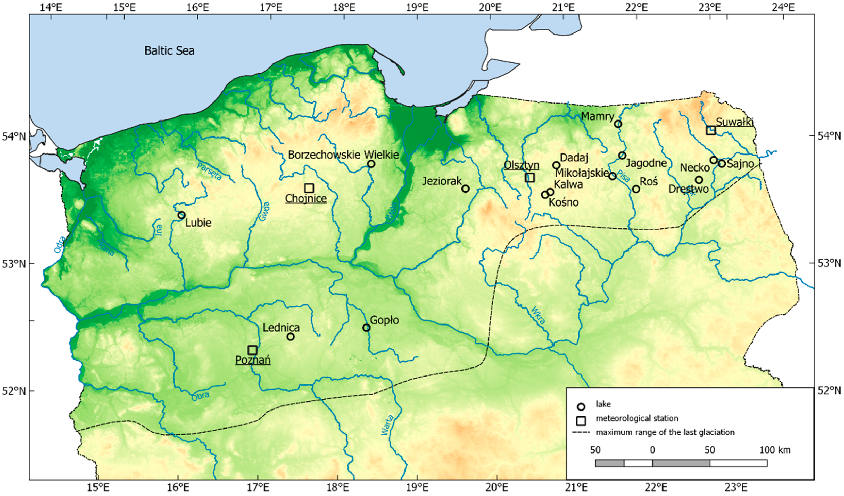
2. Materials and Methods

A total of 7081 Polish lakes have a surface area of more than 1 ha. The majority of the lakes (more than 90% [41]) is located north of the line designating the maximum range of the last glaciation.
In the research analyzed daily values of water levels in 75 lakes, and mean monthly air temperatures and atmospheric precipitation from meteorological stations of Poznań, Chojnice, Olsztyn, and Suwałki from the years 1976–2015 obtained from the Institute of Meteorology and Water Management—National Research Institute. They provided the basis for the calculation of mean monthly and annual water levels. The lakes were selected after the verification of the homogeneity of series of monthly and annual water levels by means of an Alexandersson test [42]. The critical values of the test, based on Monte Carlo simulations, were read from tables of critical values [43] at a level of α = 0.05. Then, a non-parametric Mann-Kendall test was performed, detecting trends in temporal series [44]. The results of both tests provided the basis for selection of 15 lakes for further analysis (Figure 1) the monthly and annual water level series of which are homogenous, and show no statistically significant trend.
It can be assumed that they are lakes in which water-level fluctuations are determined by physiography of the lake catchment and natural factors, including among others climatic factors such as precipitation and air temperature, shown to be affected by teleconnection patterns [45,46]. The analyzed lakes have a natural regime of water levels, as confirmed by papers [27,28,47,48]. Analyzed lakes are shallow, with average depth from 3.6 m (Gopło) to 13.7 (Kośno). Their annual mean water level amplitudes do not exceed 100 cm and range from 23 cm (Kośno) to 96 cm (Dręstwo). The highest extreme multi-year amplitudes are observed in Gopło Lake (273 cm), and the lowest ones in Kośno Lake (56 cm). These lakes are characterized by low coefficient of variation which varies from 0.02 (Jeziorak) to 0.38 (Roś) (Table 1).
The analyzed lakes represent 5 types of regimes of water levels based on the course of the water level coefficient (W), calculated as the product of mean water level in a pentad to mean water level from the multi-annual period (Table 1). Group 2b is characterized by the occurrence of high water levels (W > 1) at the turn of March and April, and low from December to March. This group included Lakes Necko and Sajno. In another type of regime (3a), Lakes Lubie, Roś, and Dręstwo were designated. High water levels are usually observed there from the second half of January to mid-May. Type 3b includes the Great Masurian Lakes. Here, high water levels in an average annual cycle occur in the period from the first half of February to mid-August, and low levels are observed in the autumn-winter period. Type 3c is represented by Lakes Kalwa, Jeziorak, Borzechowskie, and Lednica. High water levels usually occur from the second half of January to the first half of July, and low levels in the summer-autumn period. The last type of regime (4b) is represented by Lakes Kośno and Gopło. High water levels are observed from the second half of January to the turn of May and June, and low water levels begin in mid-June and persist until the first half of December [48].
The determination of dependencies of water levels in lakes on the intensity of particular teleconnection patterns involved the calculation of Pearson linear correlation coefficients. Correlation coefficients were calculated between monthly water levels in lakes and monthly NAO, AO, EA, and SCAND indices. Monthly values of teleconnection pattern indices for the years 1976–2015 were obtained from data bases of the Climate Prediction Centre (CPC), National Oceanic and Atmospheric Administration (NOAA). They were determined based on the principle component analysis of monthly anomalies of isobaric height of 500 hPa [14].
The correlation coefficients between the analyzed variables were calculated for synchronous as well as asynchronous series, e.g., the EAXI index was correlated with water levels from November to October, EAXII index with water levels from December to October, and water levels in November were correlated with the EAXII index from the previous year, etc. For each lake, a matrix was obtained, composed of 156 correlation coefficients, including correlation coefficients calculated between monthly water levels and monthly indices of particular teleconnection patterns. The statistical assessment of significance of correlation coefficients (at significance levels of p < 0.05, p < 0.1, p < 0.001) was performed by means of statistic t:
t = r n 2 1 r 2
Statistic t has Student distribution with n − 2 degrees of freedom.
At the next stage of work, values of 156 correlation coefficients for each lake were treated as variables that provided the basis for grouping of lakes by means of the Ward method. Ward [50] suggested that at each step of the analysis, the loss of information associated with merging objects was measured by the sum of squares of deviations of each object from the center of the cluster to which it belongs. At each step of grouping, the union of every possible cluster pair is considered and two clusters whose function results in the lowest increase in information loss are combined. The information loss in this method is referred to as the error sum of squares (E.S.S.), defined:
E . S . S . = i 1 n x i 2 1 n ( i 1 n x i )
where xi is the score of the i-th object. The grouping results were presented in the form of a dendrogram reflecting the structure of similarity of the analyzed group of lakes, and served for the designation of typological classes. In the paper, the number of classes was determined based on the analysis of geometry of the dendrogram and the plot of the linkage distance curve. The presented methods are commonly used in hydrometeorological research [51,52,53,54,55,56,57,58,59,60].
The mathematical-statistical processing of the analysis results employed statistical procedures included in the Excel (Microsoft) and Statistica 13 (TIBCO Software Inc.) software. The implementation of the graphic form employed the Surfer 10 (Golden Software) and Publisher (Microsoft), QGIS software. The construction of the matrix of correlation coefficients of isocorrelate was performed with the application of the kriging procedure.

3. Results

3.1. Arctic Oscillation

The analysis of the matrix of coefficients of correlation of monthly water levels with AO indices shows that the strength of correlations between the variables is temporally and spatially variable. This is suggested by results of Ward hierarchical grouping of monthly correlation coefficients. The location of particular groups of lakes to a certain degree shows regional variability (Figure 2). The first group is represented by two lakes in the north-west of the study area—Sajno and Necko. Water levels in the lakes positively correlate with AO from November to March. Statistically significant positive and synchronous correlations of AO with water levels are observed in December at a level of p < 0.05, in January (p < 0.01), and in March, in Lake Sajno even at a level of p < 0.001, and in Lake Necko p < 0.01. From April to October in Lake Sajno, and until September on Lake Necko, synchronous, but negative correlations of monthly AO indices with water levels in the lakes are observed, whereas in Lake Sajno they are statistically significant in April (p < 0.05) and May (p < 0.01), and in Lake Necko in July (p < 0.05). Asynchronous correlations of AO indices in February with water levels in September (p < 0.01) and October (p < 0.05) in Lake Sajno, and in Lake Necko from May to October (p < 0.05) and in June (p < 0.01) draw attention. The second group includes 10 lakes, in great majority located in the Masurian Lakeland. Positive correlations of AO indices with water levels from December to March are observed here. In the case of the system of the Great Masurian Lakes (Mikołajskie, Mamry, Jagodne), they are observed until April, and in March they are significant at a level of p < 0.1. In the next months, the correlations are negative, and in the majority of cases statistically non-significant. Only in August AO indices show negative statistically significant correlations with water levels in Lakes: Kośno (p < 0.01), Jagodne, Jeziorak (Figure 3), and Kalwa (p < 0.05). The research also points to asynchronous correlations, statistically significant between AO indices from January to March with water levels from May to October. In the case of Lake Jeziorak (Figure 3), AO indices in January and February correlate at a level of p < 0.01 with water levels from May to September (without June). AO indices in January show correlations with water levels in February and March (Figure 3). The third group includes lakes located in the central part of the study area: Borzechowskie, Lednica, and Gopło. In a major part of the year, negative correlations of AO indices with water level in the lakes are observed in the group. Statistically significant correlations were determined in Lake: Gopło in December (p < 0.01) and January (p < 0.05), Lednica in December (p < 0.01), and Borzechowskie in November (p < 0.05). In the case of all lakes, positive, statistically non-significant correlations were determined between AO indices and water levels in June, and in Lake Gopło from February to April, and Lednica in March and April. In all the lakes, AO indices from January to February show synchronous correlations with water levels from December to January. As shown in Figure 3, the correlations are statistically significant at a level of p < 0.001 in May, June, and September.

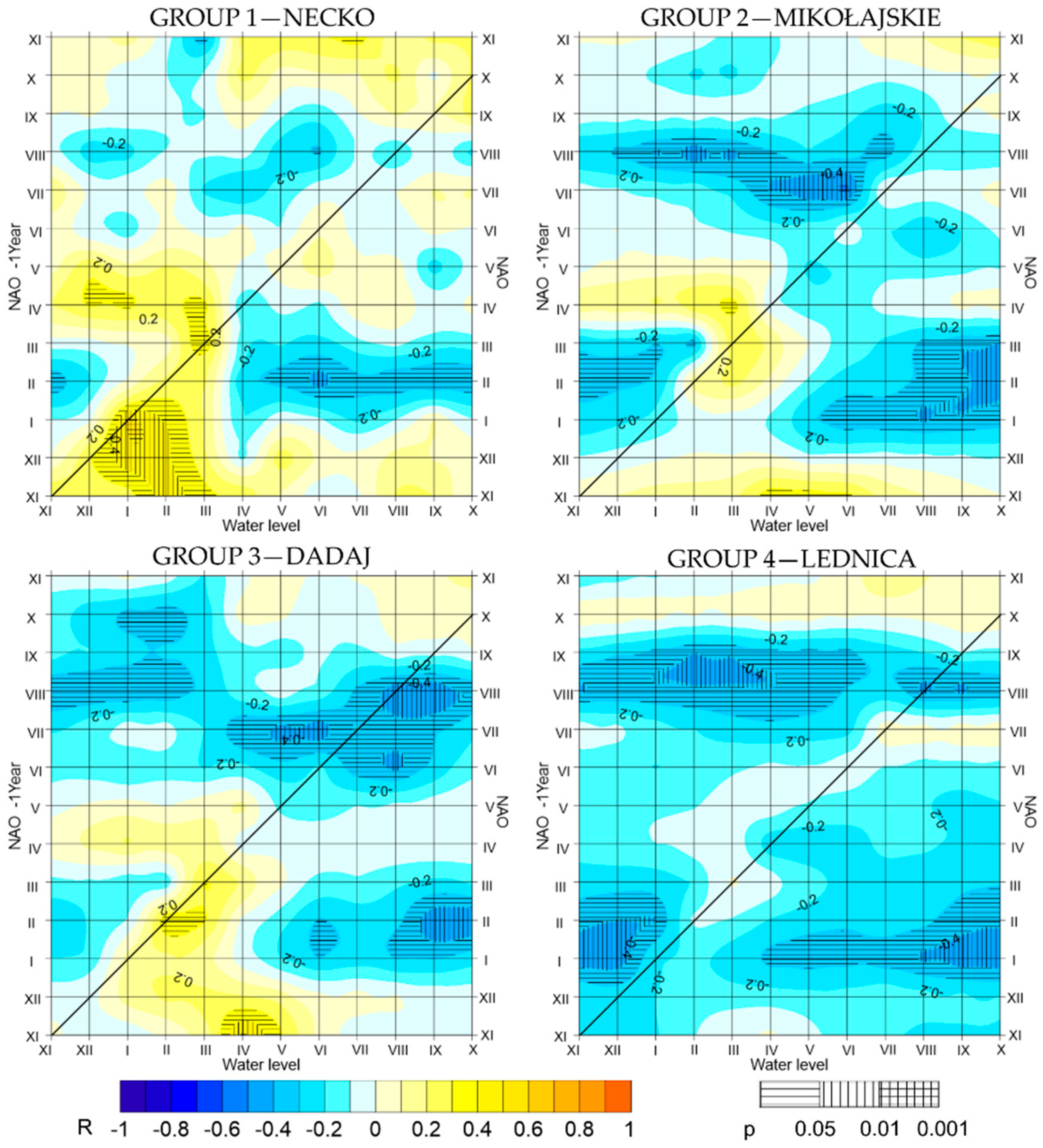
3.2. North Atlantic Oscillation

Based on grouping of coefficients of correlation between NAO and water levels in lakes, 4 groups of lakes were designated (Figure 4). Like in the case of AO, the first group included Lakes Sajno and Necko. Notice that NAO indices from November to March (Lake Necko) of April (Lake Sajno) positively correlate with water levels in those months. The group is characterized by statistically significant correlations in January. In Lake Necko they are statistically significant at a level of p < 0.001, in Lake Sajno p < 0.01, and in both lakes in March (p < 0.05). In spring and autumn, negative, statistically non-significant correlations are usually observed. An asynchronous correlation of NAO indices in February with water levels from May to October (p < 0.05) is also observed, and correlations of NAO in February are statistically significant with water levels in June at a level of p < 0.01. The second group included 5 lakes: Mikołajskie, Mamry, Jagodne, Roś, and Dręstwo (Figure 4). NAO indices usually show negative correlations with water levels in those lakes. In November and from February to April, positive statistically non-significant correlations are observed. Only in the case of Lake Jagodne, NAO indices in March correlate statistically significantly with water levels in March (p < 0.05). An asynchronous correlation is also observed between NAO indices from January to March and water levels from June to October (Figure 5). The third group also included five lakes, namely: Jeziorak, Lubie, Kośno, Kalwa, and Dadaj. They are in the western part of the Masurian Lakeland. Water levels in the lakes positively correlate with NAO from December to March, and in October. Statistically significant correlations (p < 0.05) are observed in the case of Lake Dadaj in February. From April to September, NAO indices negatively and statistically significantly correlate with water levels in August in Lakes Kośno (p < 0.05), Lubie, Dadaj, and Kalwa (p < 0.01). An asynchronous correlation of winter NAO indices with water levels in the summer-autumn period, and Nao indices in November with water levels in April and May (p < 0.01) of the following year is also observed. The fourth group included 3 lakes: Lednica, Gopło, and Borzechowskie. Throughout the year, NAO indices generally correlate negatively with water levels in lakes, statistically significantly in the case of Lakes Lednica and Gopło in August, respectively at a level of p < 0.01 and p < 0.05. Synchronous statistically significant correlations are also observed between NAO indices in January and water levels from April to October, and between NAO indices in August and water levels in lakes in September.

3.3. East Atlantic Pattern

In the case of grouping correlation coefficients of EA indices with water levels in lakes, 3 groups of lakes were designated (Figure 6). Lakes included in the groups also show quite a characteristic spatial distribution, although it is not as unambiguous as in the case of groups for AO and NAO. The first group included Lakes Sajno, Necko, and Dręstwo located in the eastern part of the study area, and lakes located in its central part: Jeziorak and Gopło. For a major part of the year, positive statistically non-significant correlations of EA indices with water levels are observed. In the spring-summer period, in some lakes (Sajno, Necko, Jeziorak, Kalwa, Dręstwo), negative correlations are recorded, but they are statistically significant only in Lake Sajno in May (p < 0.05). An asynchronous correlation of EA indices in May with water levels in summer is also observed. Statistically significant correlations were recorded in Lake Sajno in June and August (p < 0.01) as well as July (p < 0.001), in Lake Gopło in August and September (p < 0.05), and in Lake Dręstwo (Figure 7) from July to October (p < 0.05) and in August (p < 0.01). An asynchronous correlation of EA indices from December was also identified with water levels in the summer-autumn period. In Lake Dręstwo, the correlation is positive and statistically significant at a level of p < 0.05. The second group included lakes mainly located in the Masurian Lakeland, with the exception of Lake Lubie located in the western part of the study area. Like in the first group, positive, but statistically non-significant correlations are prevalent here. In the case of Lake Roś (Figure 7), EA indices in September statistically significantly correlate with water levels (p < 0.05). An asynchronous correlation is also observed between the indices in November and December and water levels from July to October (p < 0.05). The last group included 2 lakes: Borzechowskie and Lednica. Mainly positive correlations between synchronous variables are observed in this group. The correlations are statistically significant in February, July, and October (p < 0.05) in Lake Lednica (Figure 7), and in July in Lake Borzechowskie (p < 0.05). In the case of Lake Borzechowskie, also EA indices in January and March show negative, but statistically non-significant correlations with water levels in those months. In the case of both lakes, a correlation between teleconnection indices in July and water levels in lakes from August to October was also observed. In the case of Lake Lednica, the correlation was negative and statistically significant (p < 0.01).

3.4. Scandinavian Pattern

In grouping of lakes by correlation and term of occurrence of correlations of SCAND indices with water levels in the analyzed lakes, 4 groups were designated (Figure 8). One of the groups again includes Lakes Sajno and Necko (group 1). Almost throughout the year, SCAND indices negatively, but statistically non-significantly correlate with water levels in lakes. This is exemplified by the matrix of correlation coefficients for Lake Necko. SCAND indices in October correlate statistically significantly at a level of p < 0.05 with water levels in that month (Figure 9). Positive, statistically non-significant correlations are observed between SCAND indices and water levels in April and June, and in the case of Lake Sajno only in April. In both lakes, asynchronous correlations of the teleconnection indices in January with water levels in February and March were observed. Water levels in the lakes show negative, statistically significant correlations (Sajno, p < 0.05 and Necko, p < 0.001). Water levels in Lake Necko in April was positively, statistically significantly (p < 0.05) correlated with SCAND index in January. The second group includes lakes belonging to the system of the Great Masurian Lakes, interconnected with canals (Mikołajskie, Mamry, and Śniardwy). Negative correlations of SCAND indices with water levels are observed here over a major part of the year. The indices correlate statistically significantly at a level of p < 0.05 with water levels in lakes in March. Positive, but statistically non-significant correlations occur in February, and in Lakes Mikołajskie and Mamry also in July. In the case of Lakes Mamry and Jagodne, asynchronous correlations of SCAND indices in December with water levels in January, and indices in January with water levels in the lakes in February and March are also observed (p < 0.05). Group 3 includes 7 lakes (Figure 8). The matrix for Lake Kalwa is presented as an example (Figure 9). Negative, statistically non-significant correlations are generally observed between monthly SCAND indices and water levels in the lakes. Only water levels in Lake Roś in November and Lakes Kośno and Kalwa in January correlate with SCAND statistically significantly (p < 0.01). Positive correlations usually occur in the period from April to June, and in Lake Kalwa also in July. Asynchronous correlations of SCAND indices in January with water levels from February to March ae also observed, and in Lake Kalwa even until April. Negative correlations are statistically significant in all the lakes, and in the case of Lake Kalwa even at a level of p < 0.001. In group 4, water levels show positive or negative, statistically significant correlations with synchronous SCAND indices. Significant correlations are observed in the case of asynchronous series—SCAND indices in December and January with water levels in August (p < 0.05) in Lake Lednica, and in September and October (p < 0.01) in Lakes Lednica and Gopło.

3.5. Effect of Teleconnection Patterns on Air Temperature and Precipitation

Because the regime and fluctuations of water levels in lakes are largely determined by meteorological factors affecting the volume of alimentation, the analysis also covered correlations of the analyzed teleconnection patterns (AO, NAO, EA, SCAND) with air temperature and atmospheric precipitation in 4 meteorological stations: Poznań, Chojnice, Olsztyn, and Suwałki. Because the correlation analysis provided similar results for all the stations, both for air temperature and atmospheric precipitation, the results of the correlation analysis were presented only for station Olsztyn (Figure 10). The research showed that correlations of teleconnection indices with air temperature are considerably stronger than in the case of atmospheric precipitation. Changes in the intensity of monthly AO and NAO indices show high similarity in terms of both the strength and terms of the observed most significant correlations with air temperature and precipitation amount. Monthly AO and NAO indices show positive correlations with air temperature throughout the year, although the strongest, statistically significant synchronous correlations are observed from December to March (p < 0.001). Correlations with atmospheric precipitation are weaker. Positive and statistically significant synchronic correlations of AO and NAO with air temperature are observed in January (p < 0.05), and negative, statistically significant correlations from July to August. Asynchronous correlations of AO and NAO indices in January and February are determined for precipitation in August (p < 0.01).
Monthly EA indices have the strongest effect on air temperature in September and October (p < 0.001), and precipitation shows a negative, statistically significant correlation only in September (p < 0.05).
The SCAND pattern in January and February statistically significantly correlates with air temperature in those months. Positive, statistically significant correlations occur in May (p < 0.01). SCAND indices in May show asynchronous correlations with air temperature in September (p < 0.05). Statistically significant correlations of SCAND with atmospheric precipitation were also determined in the cool half-year from January to March (p < 0.01), and in October (p < 0.001).
The results of the analyses show that during warm winters in the positive phase of NAO/AO and in the negative phase of SCAND there are observed not only higher air temperatures, what cause mid-winter snowmelts and increased water supply, but also higher precipitation, what can even intensify this process. Weak correlations of EA with precipitation do not cause significant changes of lake water levels.

4. Discussion

The obtained results show that the observed correlations of teleconnection patterns with water levels in lakes are not strong, but evident. They also show temporal and spatial variability. The strongest and most significant correlations were observed in the case of AO and NAO in the winter period. This is also confirmed by findings of other authors, particularly in reference to the effect of the North Atlantic Oscillation. Nõges et al. [61] showed a strong effect of NAO on water levels in Lake Võrtsjärv in Estonia. Soja et al. [62] showed a statistically significant effect of winter NAODJFM index on water levels in Lake Neusiedl in Austria in the years 1976–2010. Sheida et al. [63] pointed to the effect of NAO on the cyclical variability of water levels in Lake Urmia in Iran, and [64] to the statistically significant negative correlation of water level in Lake Balkhash with NAO indices (winter and annual). Numerous studies evidence the effect of different teleconnection patterns on water levels and thickness of ice cover in the Great American Lakes [31,32,33,34,35,36,37]. The aforementioned papers, however, focus on a detailed analysis of single or several lakes, and do not present the regional variability of the degree and direction of correlations of water levels in different lakes, as is attempted to evidence by the authors of this paper.
Several publications can be found in the literature on the impact of the teleconnection patterns on a river flow. For instance, connections between the river flows of the Iberian peninsula and NAO indices were found [65]. The results of research indicate that NAO has a significant impact on surface water resources throughout the Iberian Peninsula during winter, and autumn, particularly in the Atlantic watershed. The authors also found the positive streamflow anomalies during extreme negative NAO phases, and vice versa. The relation between river flows of northern hemisphere and ENSO and AO was confirmed, and linear negative teleconnection of river flows in Europe to AO was identified [66].
What is more, also the correlations between flows of Mississippi River and ENSO and NAO indices [67], winter Mississippi Valley stream flow and AMO, ENSO and PNA indices [68] and winter streamflow over Romania and AO/NAO, EA, EAWR and SCAND [69] were found.
In Polish scientific literature the impact of NAO was widely described, on both meteorological and hydrological variables. The strong influence of NAO was confirmed on air temperature in cold season [70,71,72,73], precipitation [74,75], radiation and humidity conditions [76] and on the thickness of the snow cover [77,78]. In the consequence the impact of NAO on the size and dynamics of river outflow is observed. Kaczmarek [79,80] found the influence of NAO on the height of snowmelt floods of the rivers in Central Europe. In the positive phase of NAO the spring floods are usually lower than in the negative phase. It was also confirmed that NAO has impact on Warta river flows [81,82] and that there are asynchronous connections between winter NAO indices and flows of the Vistula and several Carpathian rivers [83,84]. It was also found that NAO has strong impact on the height and seasonality of the Polish rivers outflow [85,86].
Limnological research confirmed the significant correlations between NAO and water temperature [24], ice cover [25,87], and water level fluctuations [1,30]. The strongest impact of NAO on mean annual water temperature of lakes in Poland was observed in winter-spring period. Depending on the NAO phase, temperatures differ from mean values. In the positive phase they significantly exceed mean temperature, and in the negative one they are lower than mean values [24]. In case of ice phenomena, it was observed that in the negative phase they occurred later, the ice cover was thicker, and it lasted longer than average. The opposite dependence was observed in the positive phase of NAO—the duration of the ice cover phenomena was shorter than average, and the ice cover was thinner [25]. Also, the impact of NAO on lakes water level was confirmed. Stronger correlations between water levels and seasonal NAO indices were recorded in winter-spring period [1,30].
The influence of macroscale circulation types (NAO, AO, EA, EAWR, SCAND) was also analyzed in accordance to air and lakes water temperature in Poland. The strongest impact on water temperature was observed in winter for NAO and AO indices [18]. The carried-out analysis referring to Polish lakes points to regional variability of the effect of changes in the intensity of the analyzed teleconnection patterns on water levels in lakes despite a lack of such variability in reference to air temperatures and amount of atmospheric precipitation.
The lakes are located in the zone of moderate latitudes, where high water levels occur in spring due to intensified meltwater alimentation, and low levels in summer as a result of reduction of the resources due to an increase in temperature and losses related to evaporation. Despite their location practically in a single zone, the terms of occurrence of minimum and maximum values, as well as the range of their fluctuations [48], and water level amplitudes [88] are somewhat different. Therefore, the paper verifies to what degree changes in the intensity of the most important teleconnection patterns can contribute to changes in water levels in lakes. Results of the correlation analysis and Ward hierarchical grouping point to a certain correlation of changes in water levels in lakes with the intensity of particular teleconnection patterns. Results of grouping to a certain degree relate to type of lake regime designated by [48] due to the value and course of the water level coefficient representing water level fluctuations in an average annual cycle. It is the most noticeable in case of two lakes—Necko and Sajno. In each grouping they were in the same group. They are the only lakes (type 2b) which in the sequence of hydrological periods are characterized by the occurrence of very low water levels period in winter and high water levels during the period of intensified water supply caused by spring thaws with the maximum at the turn of March and April.

5. Conclusions

The applied research procedure and assessment of the importance of changes in teleconnection patterns (AO, NAO, EA and SCAND) for water level fluctuations in lakes based on the correlation analysis shows statistically significant correlations of water levels in lakes with monthly indices of the analyzed teleconnection patterns. The observed correlations are the most significant in the case of AO and NAO, and somewhat weaker for EA and SCAND. These teleconnection patterns particularly affect air temperature, and to a lower degree precipitation. Therefore, they may indirectly affect the conditions of alimentation of lakes. In positive phases of AO and NAO during warmer winters, the type of alimentation changes from nival to rain. Due to winter snowmelts, also more frequent in the period, the alimentation increases, and water levels in lakes are higher. The existence of very significant negative asynchronous correlations of AO and NAO indices in February with the amount of precipitation in August is interesting. Lower precipitation in the summer period may be reflected in lower summer-autumn water levels in lakes, which would confirm similar correlations of AO and NAO indices in February with water levels in lakes in the period. The weakest correlations with water levels in lakes were determined in the case of EA. Although in the positive phase, particularly in the summer-autumn period, the teleconnection pattern contributes to an increase in air temperature and a decrease in atmospheric precipitation, it is reflected in changes in water levels in lakes to a low degree. The effect of changes in the intensity of SCAND on water levels is observed, however, particularly in lakes located in the eastern, cooler part of the study area. In the positive phase of SCAND, in the winter-spring period, from January to March, atmospheric precipitation and air temperature (particularly in February) are considerably lower. As a consequence, alimentation of lakes decreases, and water levels in the lakes also decrease in the period.
In the case of such research, aimed at the determination of correlations between variables, it is very important to previously verify the hydrometric material for the purpose of avoidance of incidental dependencies. For this purpose, all lakes showing anthropogenic disturbances in the water level regime, lack of homogeneity of observation series, or statistically significant tendencies in the analyzed variables were eliminated from the analysis. It should be remembered, however, that linear correlation is not a resistant measure [89]. This means that untypical observations (so-called outliers) may considerably affect the value of the correlation coefficient. Moreover, the analysis of the obtained coefficients does not permit simultaneous determination of the strength of correlation between hydrological variables and indices of particular teleconnection patterns. Statistically significant correlation coefficients only point to the same (positive correlations) or opposite (negative correlations) direction of correlation. In the scope of continuation of research on the effect of different teleconnection patterns, it seems necessary to introduce more advanced statistical analyses. An attempt of such research was conducted by among others [90]—the authors analyzed the effect of variability of climate features (expressed in among others NAO and ENSO indices) on values of the SPEI index (Standard Precipitation Evapotranspiration Index) in the Yangtze River Basin, with the application of combined distribution calculated on the basis of Copula functions. Even more advanced computational methods (like machine learning and artificial neural networks) can be used to predict future values of given hydro- and meteorological variables. These methods were used for instance to forecast runoff values for the effective reservoir management [91], to predict evaporation [92,93] or to establish a rainfall-runoff models for forecasting the river flow [94,95,96,97].
To sum up, climate conditions variability has an impact on lakes water level fluctuations. In the time of progressing climate change, particular attention should be paid to the fact that Poland is one of the countries with the smallest water resources in Europe [98]. Therefore, in the light of the declining lakes water resources observed [99], it is really important to monitor the fluctuations in lakes water levels and to determine their causes for the purposes of rational and effective water management.

Author Contributions

Conceptualization, K.P., D.W., A.P.; methodology, D.W.; software, K.P., A.P.; validation, K.P., A.P.; formal analysis, K.P, A.P.; investigation, K.P., D.W., A.P.; resources, K.P.; writing—original draft preparation, K.P., A.P.; writing—review and editing, K.P., A.P., D.W.; visualization, K.P., A.P.

Funding

This research received no external funding.

Conflicts of Interest

The authors declare no conflict of interest.

References

  1. Wrzesiński, D.; Ptak, M.; Plewa, K. Effect of the North Atlantic Oscillation on water level fluctuations in lakes of northern Poland. Geographia Polonica 2018, 91, 243–259. [Google Scholar] [CrossRef]
  2. Schaefer, K.; Denning, A.S.; Leonard, O. The winter Arctic Oscillation and the timing of snowmelt in Europe. Geophys. Res. Lett. 2004, 31. [Google Scholar] [CrossRef] [Green Version]
  3. Jevrejeva, S.; Moore, J.C.; Grinsted, A. Influence of the Arctic Oscillation and El Niño-Southern Oscillation (ENSO) on ice conditions in the Baltic Sea: The wavelet approach. J. Geophys. Res. Atmos. 2003, 108. [Google Scholar] [CrossRef]
  4. Wang, D.; Wang, C.; Yang, X.; Lu, J. Winter Northern Hemisphere surface air temperature variability associated with the Arctic Oscillation and North Atlantic Oscillation. Geophys. Res. Lett. 2005, 32. [Google Scholar] [CrossRef] [Green Version]
  5. Trigo, R.M.; Osborn, T.J.; Corte-Real, J.M. The North Atlantic Oscillation influence on Europe: Climate impacts and associated physical mechanisms. Clim. Res. 2002, 20, 9–17. [Google Scholar] [CrossRef]
  6. Hurrell, J.W.; Kushnir, Y.; Ottersen, G.; Visbeck, M. An overview of the North Atlantic oscillation. In The North Atlantic Oscillation, Hurrell, J.W.; Kushnir, Y., Ottersen, G., Visbeck, M., Eds.; American Geophysical Union (AGU): Washington, DC, USA, 2003. [Google Scholar] [CrossRef]
  7. Trigo, R.M.; Pozo-Vázquez, D.; Osborn, T.J.; Castro-Díez, Y.; Gámiz-Fortis, S.; Esteban-Parra, M.J. North Atlantic Oscillation influence on precipitation, river flow and water resources in the Iberian Peninsula. Int. J. Climatol. 2004, 24, 925–944. [Google Scholar] [CrossRef]
  8. Moore, G.W.K.; Renfrew, I.A. Cold European winters: Interplay between the NAO and the East Atlantic mode. Atmos. Sci. Lett. 2012, 13, 1–8. [Google Scholar] [CrossRef]
  9. Knežević, S.; Tošić, I.; Unkašević, M.; Pejanović, G. The influence of the East Atlantic Oscillation to climate indices based on the daily minimum temperatures in Serbia. Theor. Appl. Climatol. 2014, 116, 435–446. [Google Scholar] [CrossRef]
  10. Casanueva, A.; Rodríguez-Puebla, C.; Frías, M.D.; González-Reviriego, N. Variability of extreme precipitation over Europe and its relationships with teleconnection patterns. Hydrol. Earth Syst. Sci. 2014, 18, 709–725. [Google Scholar] [CrossRef] [Green Version]
  11. Bednorz, E.; Wibig, J. Snow depth in eastern Europe in relation to circulation patterns. Ann. Glaciol. 2008, 48, 135–149. [Google Scholar] [CrossRef] [Green Version]
  12. Comas-Bru, L.; Mcdermott, F. Impacts of the EA and SCA patterns on the European twentieth century NAO—Winter climate relationship. Q. J. R. Meteorolog. Soc. 2014, 140, 354–363. [Google Scholar] [CrossRef]
  13. Higgins, R.W.; Leetmaa, A.; Kousky, V.E. Relationships between climate variability and winter temperature extremes in the United States. J. Clim. 2002, 15, 1555–1572. [Google Scholar] [CrossRef]
  14. Barnston, A.G.; Livezey, R.E. Classification, seasonality and persistence of low-frequency atmospheric circulation patterns. Mon Weather Rev. 1987, 115, 1083–1126. [Google Scholar] [CrossRef]
  15. Wibig, J. Precipitation in Europe in relation to circulation patterns at the 500 hPa level. Int. J. Climatol. 1999, 19, 253–269. [Google Scholar] [CrossRef]
  16. Tomczyk, A.M. Impact of macro-scale circulation types on the occurrence of frosty days in Poland. Bull. Geogr. Phys. Geog. Ser. 2015, 9, 55–65. [Google Scholar] [CrossRef] [Green Version]
  17. Tomczyk, A.M.; Szyga-Pluta, K.; Bednorz, E. The effect of macro-scale circulation types on the length of the growing season in Poland. Meteorol. Atmos. Phys. 2018, 1–11. [Google Scholar] [CrossRef]
  18. Ptak, M.; Tomczyk, A.; Wrzesiński, D. Effect of teleconnection patterns on changes in water temperature in Polish lakes. Atmosphere 2018, 9, 66. [Google Scholar] [CrossRef]
  19. Bednorz, E. Snow cover in western Poland and macro-scale circulation conditions. Int. J. Climatol. 2002, 22, 533–541. [Google Scholar] [CrossRef]
  20. Bednorz, E. Snow cover in eastern Europe in relation to temperature, precipitation and circulation. Int. J. Climatol. 2004, 24, 591–601. [Google Scholar] [CrossRef]
  21. Skowron, R. Changeability of the ice cover on the lakes of northern Poland in the light of climatic changes. Bull. Geogr. Phys. Geog. Ser. 2009, 1, 103–123. [Google Scholar] [CrossRef]
  22. Girjatowicz, J.P. Effects of the North Atlantic Oscillation on water temperature in southern Baltic coastal lakes. Annales de Limnologie—Int. J. Limnol. 2011, 47, 73–84. [Google Scholar] [CrossRef]
  23. Bernhardt, J.; Engelhardt, C.; Kirillin, G.; Matschullat, J. Lake ice phenology in Berlin-Brandenburg from 1947–2007: Observations and model hindcasts. Clim. Change 2012, 112, 791–817. [Google Scholar] [CrossRef]
  24. Wrzesiński, D.; Choiński, A.; Ptak, M. Effect of the North Atlantic Oscillation on the thermal characteristics of lakes in Poland. Act. Geophys. 2015, 63, 863–883. [Google Scholar] [CrossRef]
  25. Wrzesiński, D.; Choiński, A.; Ptak, M.; Skowron, R. Effect of the North Atlantic Oscillation on the Pattern of Lake Ice Phenology in Poland. Act. Geophys. 2015, 63, 1664–1684. [Google Scholar] [CrossRef] [Green Version]
  26. Górniak, A.; Piekarski, K. Seasonal and multiannual changes of water levels in lakes of northeastern Poland. Pol. J. Environ. Stud. 2002, 11, 349–354. [Google Scholar]
  27. Wrzesiński, D.; Ptak, M. Water level changes in Polish lakes during 1976–2010. J. Geog. Sci. 2016, 26, 83–101. [Google Scholar] [CrossRef]
  28. Wrzesiński, D.; Plewa, K. Stability of the water levels regime on the lakes in Poland. Badania Fizjograficzne Seria A Geografia Fizyczna 2016, A67, 305–316. [Google Scholar] [CrossRef]
  29. Plewa, K.; Wrzesiński, D. Wpływ Oscylacji Północnoatlantyckiej na zmiany stabilności reżimu stanów wody jezior w Polsce. Badania Fizjograficzne Seria A Geografia Fizyczna 2017, A68, 127–138. [Google Scholar] [CrossRef]
  30. Wrzesiński, D.; Ptak, M. An investigation of water level fluctuations in Polish lakes in various phases of the winter North Atlantic Oscillation. Geol. Geophys. Environ. 2017, 43. [Google Scholar] [CrossRef]
  31. Assel, R.; Rodionov, S. Atmospheric teleconnections for annual maximum ice cover on the Laurentian Great Lakes. Int. J. Climatol. 1998, 18, 425–442. [Google Scholar] [CrossRef]
  32. Ghanbari, R.N.; Bravo, H.R. Coherence between atmospheric teleconnections, Great Lakes water levels, and regional climate. Adv. Water Resour. 2008, 31, 1284–1298. [Google Scholar] [CrossRef]
  33. Wang, J.; Bai, X.; Hu, H.; Clites, A.; Colton, M.; Lofgren, B. Temporal and spatial variability of Great Lakes ice cover, 1973–2010. J. Clim. 2012, 25, 1318–1329. [Google Scholar] [CrossRef]
  34. Biron, S.; Assani, A.A.; Frenette, J.J.; Massicotte, P. Comparison of Lake Ontario and St. Lawrence River hydrologic droughts and their relationship to climate indices. Water Resour. Res. 2014, 50, 1396–1409. [Google Scholar] [CrossRef]
  35. Assani, A.A.; Landry, R.; Azouaoui, O.; Massicotte, P.; Gratton, D. Comparison of the characteristics (frequency and timing) of drought and wetness indices of annual mean water levels in the five North American Great Lakes. Water Resour. Manag. 2016, 30, 359–373. [Google Scholar] [CrossRef]
  36. Hewitt, B.; Lopez, L.; Gaibisels, K.; Murdoch, A.; Higgins, S.; Magnuson, J.; Paterson, A.; Rusak, J.; Yao, H.; Sharma, S. Historical trends, drivers, and future projections of ice phenology in small north temperate lakes in the Laurentian Great Lakes Region. Water 2018, 10, 70. [Google Scholar] [CrossRef]
  37. Fu, W.; Steinschneider, S. A Diagnostic-Predictive Assessment of Winter Precipitation over the Laurentian Great Lakes: Effects of ENSO and Other Teleconnections. J. Hydrometeorol. 2019, 20, 117–137. [Google Scholar] [CrossRef]
  38. Ghanbari, R.N.; Bravo, H.R.; Magnuson, J.J.; Hyzer, W.G.; Benson, B.J. Coherence between lake ice cover, local climate and teleconnections (Lake Mendota, Wisconsin). J. Hydrol. 2009, 374, 282–293. [Google Scholar] [CrossRef]
  39. Wang, H.; Pan, Y.; Chen, Y. Impacts of regional climate and teleconnection on hydrological change in the Bosten Lake Basin, arid region of northwestern China. J. Water Clim. Chang. 2018, 9, 74–88. [Google Scholar] [CrossRef]
  40. Belete, M.; Diekkrüger, B.; Roehrig, J. Linkage between water level dynamics and climate variability: The case of Lake Hawassa hydrology and ENSO phenomena. Climate 2017, 5, 21. [Google Scholar] [CrossRef]
  41. Choiński, A. Katalog jezior Polski; Wydawnictwo Naukowe Uniwersytetu im; Adama Mickiewicza: Poznań, Poland, 2006. [Google Scholar]
  42. Alexandersson, H.; Moberg, A. Homogenization of Swedish temperature data. Part I: Homogeneity test for linear trends. Int. J. Climatol. 1997, 17, 25–34. [Google Scholar] [CrossRef]
  43. Khaliq, M.N.; Ouarda, T.B. Short Communication on the critical values of the standard normal homogeneity test (SNHT). Int. J. Climatol. 2007, 27, 681–687. [Google Scholar] [CrossRef]
  44. Salmi, T.; Määttä, A.; Anttila, P.; Ruoho-Airola, T.; Amnell, T. Detecting Trends of Annual Values of Atmospheric Pollutants by the Mann-Kendall Test and Sen’s Slope Estimates—The Excel Template Application MAKESENS; Finnish Meteorological Institute: Helsinki, Finland, 2002. [Google Scholar]
  45. Niedźwiedź, T.; Twardosz, R.; Walanus, A. Long-term variability of precipitation series in east central Europe in relation to circulation patterns. Theor. Appl. Climatol. 2009, 98, 337–350. [Google Scholar] [CrossRef]
  46. Rust, H.W.; Richling, A.; Bissolli, P.; Ulbrich, U. Linking teleconnection patterns to European temperature—A multiple linear regression model. Meteorol. Z. 2015, 24, 411–423. [Google Scholar] [CrossRef]
  47. Plewa, K.; Wrzesiński, D.; Ptak, M. Reżim stanów wody wybranych jezior Pojezierza Wielkopolsko-Kujawskiego. Badania Fizjograficzne Seria A—Geografia Fizyczna 2015, A66, 131–142. [Google Scholar] [CrossRef]
  48. Plewa, K. Typy przebiegu pentadowych współczynników stanu wody jezior Niżu Polskiego. Badania Fizjograficzne Seria A—Geografia Fizyczna 2018, A69, 161–177. [Google Scholar]
  49. Czarnecka, H. Atlas podziału hydrograficznego Polski: Zestawienia zlewni; Instytut Meteorologii i Gospodarki Wodnej: Warszawa, Poland, 2005. [Google Scholar]
  50. Ward, J.H. Hierarchical grouping to optimize an objective function. J. Am. Stat. Assoc. 1963, 58, 236–244. [Google Scholar] [CrossRef]
  51. Berhanu, B.; Seleshi, Y.; Demisse, S.; Melesse, A. Flow regime classification and hydrological characterization: A case study of Ethiopian rivers. In Water; 2015; Volume 7, pp. 3149–3165. [Google Scholar]
  52. Isik, S.; Turan, A.; Dogan, E. Classification of river yields in Turkey with cluster analysis. Presented at EWRI 2006 World Environmental and Water Resources Congress, Omaha, NE, USA, 21–35 May 2006. [Google Scholar]
  53. Isik, S.; Singh, V.P. Hydrologic regionalization of watersheds in Turkey. J. Hydrol. Eng. 2008, 13, 824–834. [Google Scholar] [CrossRef]
  54. Mishra, S.; Saravanan, C.; Dwivedi, V.K.; Pathak, K.K. Discovering flood recession pattern in hydrological time series data mining during the post monsoon period. Int. J. Comput. Appl. Technol. 2014, 90, 35–44. [Google Scholar] [CrossRef]
  55. Zhang, Y.; Arthington, A.H.; Bunn, S.E.; Mackay, S.; Xia, J.; Kennard, M. Classification of flow regimes for environmental flow assessment in regulated rivers: The Huai River Basin, China. River Res. Appl. 2012, 28, 989–1005. [Google Scholar] [CrossRef]
  56. Jeneiová, K.; Kohnová, S.; Sabo, M. Detecting trends in the annual maximum discharges in the Vah River Basin, Slovakia. Acta Silvatica et Lignaria Hungarica 2014, 10, 133–144. [Google Scholar] [CrossRef]
  57. Firat, M.; Dikbas, F.; Koç, A.C.; Gungor, M. Missing data analysis and homogeneity test for Turkish precipitation series. Sadhana 2010, 35, 707. [Google Scholar] [CrossRef]
  58. Bormann, H.; Pinter, N.; Elfert, S. Hydrological signatures of flood trends on German rivers: Flood frequencies, flood heights and specific stages. J. Hydrol. 2011, 404, 50–66. [Google Scholar] [CrossRef]
  59. Fathian, F.; Dehghan, Z.; Bazrkar, M.H.; Eslamian, S. Trends in hydrological and climatic variables affected by four variations of the Mann-Kendall approach in Urmia Lake basin, Iran. Hydrol. Sci. J. 2016, 61, 892–904. [Google Scholar] [CrossRef]
  60. Mello, C.R.D.; Norton, L.D.; Curi, N.; Yanagi, S.N.M. Sea surface temperature (SST) and rainfall erosivity in the Upper Grande River Basin, Southeast Brazil. Ciência e Agrotecnologia 2012, 36, 53–59. [Google Scholar] [CrossRef]
  61. Nõges, T.; Nõges, P.; Laugaste, R. Water level as the mediator between climate change and phytoplankton composition in a large shallow temperate lake. Hydrobiologia 2003, 506, 257–263. [Google Scholar] [CrossRef]
  62. Soja, G.; Züger, J.; Knoflacher, M.; Kinner, P.; Soja, A.M. Climate impacts on water balance of a shallow steppe lake in Eastern Austria (Lake Neusiedl). J. Hydrol. 2013, 480, 115–124. [Google Scholar] [CrossRef]
  63. Sheida, J.; Hamidi, S.A.; Ghanbari, R.N. Climate variability and anthropogenic effects on Lake Urmia water level fluctuations, northwestern Iran. Hydrol. Sci. J. 2016, 61, 1759–1769. [Google Scholar] [CrossRef]
  64. Krupa, E.; Slyvinskiy, G.; Barinova, S. The Effect of Climatic Factors on the Long-term Dynamics of Aquatic Ecosystem of the Balkhash Lake (Kazakhstan, Central Asia). Adv. Stud. Biol. 2014, 6, 3. [Google Scholar] [CrossRef]
  65. Lorenzo-Lacruz, J.; Vicente-Serrano, S.M.; López-Moreno, J.I.; González-Hidalgo, J.C.; Morán-Tejeda, E. The response of Iberian rivers to the North Atlantic Oscillation. Hydrol. Earth Syst. Sci. 2011, 15, 2581–2597. [Google Scholar] [CrossRef] [Green Version]
  66. Fleming, S.W.; Dahlke, H.E. Parabolic northern-hemisphere river flow teleconnections to El Niño-Southern Oscillation and the Arctic Oscillation. Environ. Res. Lett. 2014, 9. [Google Scholar] [CrossRef]
  67. Enfield, D.B.; Mestas-Nuñez, A.M.; Trimble, P.J. The Atlantic multidecadal oscillation and its relation to rainfall and river flows in the continental US. Geophys. Res. Lett. 2001, 28, 2077–2080. [Google Scholar] [CrossRef]
  68. Rogers, J.C.; Coleman, J.S. Interactions between the Atlantic Multidecadal Oscillation, El Nino/La Nina, and the PNA in winter Mississippi valley stream flow. Geophys. Res. Lett. 2003, 30. [Google Scholar] [CrossRef]
  69. Ionita, M.; Chelcea, S.; Rimbu, N.; Adler, M.J. Spatial and temporal variability of winter streamflow over Romania and its relationship to large-scale atmospheric circulation. J. Hydrol. 2014, 519, 1339–1349. [Google Scholar] [CrossRef]
  70. Marsz, A.A.; Styszyńska, A. Oscylacja Północnego Atlantyku a temperatura powietrza nad Polską; Wydaw Uczelniane WSM: Warsaw, Poland, 2001. [Google Scholar]
  71. Kożuchowski, K.; Degirmendžic, J. Wskaźniki cyrkulacji a temperatura powietrza w Polsce. In Oscylacja Północnego Atlantyku i jej rola w kształtowaniu zmienności warunków klimatycznych i hydrologicznych Polski; Marsz, A.A., Styszyńska, A., Eds.; Akad Morska: Gdynia, Poland, 2002. [Google Scholar]
  72. Niedźwiedź, T. Relacje między NAO a wskaźnikami cyrkulacji nad Polską. In Oscylacja Północnego Atlantyku i jej rola w kształtowaniu zmienności warunków klimatycznych i hydrologicznych Polski; Marsz, A.A., Styszyńska, A., Eds.; Akad Morska: Gdynia, Poland, 2002. [Google Scholar]
  73. Przybylak, R.; Wójcik, G.; Marciniak, K. Wpływ Oscylacji Północnoatlantyckiej i Arktycznej na warunki termiczne chłodnej pory roku w Polsce w XVI–XX wiekach. Przegl. Geofiz 2003, 1–2, 61–74. [Google Scholar]
  74. Styszyńska, A. Oscylacja Północnego Atlantyku a opady na obszarze Polski. Pr Stud. Geogr. 2001, 29, 232–241. [Google Scholar]
  75. Wibig, J. Wpływ cyrkulacji atmosferycznej na rozkład przestrzenny anomalii temperatury i opadów w Europie; Wydawnictwo UŁ: Łódź, Poland, 2001. [Google Scholar]
  76. Bryś, K.; Bryś, T. Wpływ Oscylacji Północnoatlantyckiej na zmienność warunków wilgotnościowych, radiacyjnych, dynamicznych i ewaporacyjnych we Wrocławiu-Swojcu w latach 1946–2000. In Oscylacja Północnego Atlantyku i jej rola w kształtowaniu zmienności warunków klimatycznych i hydrologicznych Polski; Marsz, A.A., Styszyńska, A., Eds.; Akad Morska: Gdynia, Poland, 2002. [Google Scholar]
  77. Falarz, M. Snow cover variability in Poland in relations to macro- and mesoscale atmospheric circulation in the twentieth century. Int. J. Climatol. 2007, 27, 2069–2081. [Google Scholar] [CrossRef]
  78. Bednorz, E. Wpływ sytuacji barycznych na występowanie pokrywy śnieżnej na obszarach nizinnych środkowej Europy; Wydawnictwo Naukowe UAM: Poznań, Poland, 2009. [Google Scholar]
  79. Kaczmarek, Z. Wpływ Oscylacji Północnoatlantyckiej na przepływy rzek europejskich. In Oscylacja Północnego Atlantyku i jej rola w kształtowaniu zmienności warunków klimatycznych i hydrologicznych Polski; Marsz, A.A., Styszyńska, A., Eds.; Akad Morska: Gdynia, Poland, 2002. [Google Scholar]
  80. Kaczmarek, Z. The Impact Climate Variability on Flood Risk in Poland. Risk Anal. 2003, 23, 559–566. [Google Scholar] [CrossRef]
  81. Styszyńska, A. Związki między przepływem Warty w Poznaniu a zimowymi wskaźnikami NAO w okresie 1865–2000. In Oscylacja Północnego Atlantyku i jej rola w kształtowaniu zmienności warunków klimatycznych i hydrologicznych Polski; Marsz, A.A., Styszyńska, A., Eds.; Akad Morska: Gdynia, Poland, 2002. [Google Scholar]
  82. Styszyńska, A.; Tamulewicz, J. Warta river discharges in Poznań and atmospheric circulation in the North Atlantic region. Quaestiones Geographicae 2004, 23, 61–81. [Google Scholar]
  83. Pociask-Karteczka, J.; Nieckarz, Z.; Limanówka, D. The North Atlantic Oscillation impact on hydrological regime in Polish Carpathians. In Interdisciplinary Approaches in Small Catchment Hydrology: Monitoring and Research; FRIEND International Conference: Demanovska Dolina, Slovakia, 2002; p. 225230. [Google Scholar]
  84. Pociask-Karteczka, J.; Limanówka, D.; Nieckarz, Z. Wpływ Oscylacji Północnoatlantyckiej na przepływy rzek karpackich (1951–2000). Fol. Geogr. Ser. Geographia-Physica 2002–2003, 33–34, 89–104. [Google Scholar]
  85. Wrzesiński, D. Regional differences in the influence of the North Atlantic Oscillation on seasonal river runoff in Poland. Quaestiones Geographicae 2011, 30, 127–136. [Google Scholar] [CrossRef] [Green Version]
  86. Wrzesiński, D.; Paluszkiewicz, R. Spatial differences in the impact of the North Atlantic Oscillation on the flow of rivers in Europe. Hydrol. Res. 2011, 42, 30–39. [Google Scholar] [CrossRef]
  87. Wrzesiński, D.; Ptak, M.; Baczyńska, A. Effect of the North Atlantic Oscillation on ice phenomena on selected lakes in Poland over the years 1961–2010. Quaestiones Geographicae 2013, 32, 119–128. [Google Scholar] [CrossRef]
  88. Plewa, K.; Wrzesiński, D.; Baczyńska, A. Przestrzenne i czasowe zróżnicowanie amplitud stanów wody jezior w Polsce w latach 1981–2015. Badania Fizjograficzne Seria A—Geografia Fizyczna 2017, A68, 115–126. [Google Scholar] [CrossRef]
  89. Gurgul, P.; Syrek, R. Zastosowanie mieszanki kopul do modelowania współzależności pomiędzy wybranymi sektorami gospodarki. Ekonomia Menedżerska 2009, 6, 129–139. [Google Scholar]
  90. Huang, T.; Ligang, X.; Hongxiang, F. Drought Characteristics and Its Response to the Global Climate Variability in the Yangtze River Basin, China. Water 2019, 11, 13. [Google Scholar] [CrossRef]
  91. Wang, W.C.; Chau, K.W.; Qiu, L.; Chen, Y.B. Improving forecasting accuracy of medium and long-term runoff using artificial neural network based on EEMD decomposition. Environ. Res. 2015, 139, 46–54. [Google Scholar] [CrossRef] [PubMed]
  92. Ghorbani, M.A.; Kazempour, R.; Chau, K.W.; Shamshirband, S.; Ghazvinei, P.T. Forecasting pan evaporation with an integrated artificial neural network quantum-behaved particle swarm optimization model: A case study in Talesh, Northern Iran. Eng. Appl. Comput. Fluid Mech. 2018, 12, 724–737. [Google Scholar] [CrossRef]
  93. Moazenzadeh, R.; Mohammadi, B.; Shamshirband, S.; Chau, K.W. Coupling a firefly algorithm with support vector regression to predict evaporation in northern Iran. Eng. Appl. Comput. Fluid Mech. 2018, 12, 584–597. [Google Scholar] [CrossRef] [Green Version]
  94. Wu, C.L.; Chau, K.W. Rainfall–runoff modeling using artificial neural network coupled with singular spectrum analysis. J. Hydrol. 2011, 399, 394–409. [Google Scholar] [CrossRef]
  95. Petty, T.R.; Dhingra, P. Streamflow Hydrology Estimate Using Machine Learning (SHEM). J. Am. Water Resour. Assoc. 2017, 54, 55–68. [Google Scholar] [CrossRef]
  96. Tian, Y.; Xu, Y.P.; Yang, Z.; Wang, G.; Zhu, Q. Integration of a Parsimonious Hydrological Model with Recurrent Neural Networks for Improved Streamflow Forecasting. Water 2018, 10, 1655. [Google Scholar] [CrossRef]
  97. Yaseen, Z.M.; Sulaiman, S.O.; Deo, R.C.; Chau, K.W. An enhanced extreme learning machine model for river flow forecasting: State-of-the-art, practical applications in water resource engineering area and future research direction. J. Hydrol. 2019, 569, 387–408. [Google Scholar] [CrossRef]
  98. Kowalczak, P.; Farat, R.; Kepinska-Kasprzak, M.; Kuznicka, M.; Mager, P. Hierarchy of aerial small water retention need. Materiały Badawcze Seria Gospodarka Wodna a Ochrona Wód 1997, 19, 90. [Google Scholar]
  99. Nowak, B.; Ptak, M. Potential use of lakes as a component of small retention in Wielkopolska. In Proceedings of the 10th Conference on Interdisciplinary Problems in Environmental Protection and Engineering EKO-DOK 2018, Polanica-Zdrój, Poland, 16–18 April 2018; EDP Sciences: Les Ulis, France, 2018. [Google Scholar] [CrossRef]
Figure 1. Location of the lakes.
Water 11 01330 g001
Figure 2. Dendrogram of grouping lakes by values of correlation coefficients of monthly AO indices with monthly water levels and the plot of the linkage distance (A); Spatial distribution of lakes in the performed grouping (B).
Water 11 01330 g002
Figure 3. Matrices of coefficients of correlation for selected lakes in the designated groups (AO).
Water 11 01330 g003
Figure 4. Dendrogram of grouping lakes by values of correlation coefficients of monthly NAO indices with monthly water levels and the plot of the linkage distance (A); Spatial distribution of lakes in the performed grouping (B).
Water 11 01330 g004
Figure 5. Matrices of coefficients of correlation for selected lakes in the designated groups (NAO).
Water 11 01330 g005
Figure 6. Dendrogram of grouping lakes by values of correlation coefficients of monthly EA indices with monthly water levels and the plot of the linkage distance (A); Spatial distribution of lakes in the performed grouping (B).
Water 11 01330 g006
Figure 7. Matrices of coefficients of correlation for selected lakes in the designated groups (EA).
Water 11 01330 g007
Figure 8. Dendrogram of grouping lakes by values of correlation coefficients of monthly SCAND indices with monthly water levels and the plot of the linkage distance (A); Spatial distribution of lakes in the performed grouping (B).
Water 11 01330 g008
Figure 9. Matrices of coefficients of correlation for selected lakes in the designated groups (SCAND).
Water 11 01330 g009
Figure 10. Matrices of coefficients of correlation for temperature and precipitation in Olsztyn station in considered circulation types.
Water 11 01330 g010
Table 1. Morphometric data of the studied lakes, as well as their water level amplitudes and type of regime of water levels.
LakeArea (ha) 1Volume (thousand m3) 1Average Depth (m) 1Maximum Depth (m) 1Coefficient of Variation (Cv)Amplitudes of Water Level (cm)Type of Regime 2Area of Catchment (km2) 3Schindler Index (m−1)Ohle Index (-)Elements of the Water Balance of Lake CatchmentWater Exchange Rate α
Annual MaxAnnual MeanExtreme Multi-YearOutflow (mm) 4Precipitation (mm) 5
Lubie1487.5169,880.511.646.20.0616571843a780.864.6052.492156600.99
Lednica325.024,397.07.015.10.173118581863c43.141.7713.271005400.18
Gopło2121.578,497.03.616.60.152226872734b1151.2614.6754.27955051.39
Borzechowskie240.027,002.011.043.00.1324929743c17.250.647.192106300.13
Jeziorak3152.5141,594.24.112.90.0177644903c325.282.3010.321906200.44
Kośno562.575,767.313.744.60.0635623564b236.733.1242.092006000.62
Kalwa561.039,468.67.031.70.0875833763b75.701.9213.491956000.37
Dadaj975.0120,784.212.039.80.189141711544b340.082.8234.882006150.56
Mikołajskie424.055,739.711.225.90.2246438953b1814.8732.56428.042005956.51
Mamry9851.01,003,367.59.843.80.1066239923b618.520.626.281806000.11
Jagodne872.582,705.28.737.40.1116239953b518.676.2759.452056001.29
Roś1808.5152,924.98.131.80.378140881773a3033.0719.83167.712156004.26
Dręstwo549.042,734.68.525.00.180146962083a827.8719.37150.801605903.10
Necko400.040,561.410.125.00.028106461322b893.5422.03223.391806003.97
Sajno494.052,446.810.027.00.116161901832b959.7818.30194.291806003.29
Elaboration based on: 1 [41], 2 [48], 3 [49], 4 based on the data from 235 precipitation gauges, 5 based on the data from 516 water gauges.

