Article

Sediment Identification Using Machine Learning Classifiers in a Mixed-Texture Dredge Pit of Louisiana Shelf for Coastal Restoration

1
Department of Oceanography and Coastal Sciences, Louisiana State University, Baton Rouge, LA 70803, USA
2
Coastal Studies Institute, Louisiana State University, Baton Rouge, LA 70803, USA
3
Department of Experimental Statistics, Louisiana State University, Baton Rouge, LA 70803, USA
4
Department of Geography and Anthropology, Louisiana State University, Baton Rouge, LA 70803, USA
*
Author to whom correspondence should be addressed.
Water 2019, 11(6), 1257; https://doi.org/10.3390/w11061257
Submission received: 18 May 2019 / Revised: 10 June 2019 / Accepted: 11 June 2019 / Published: 15 June 2019

Abstract

:
Machine learning classifiers have been rarely used for the identification of seafloor sediment types in the rapidly changing dredge pits for coastal restoration. Our study uses multiple machine learning classifiers to identify the sediment types of the Caminada dredge pit in the eastern part of the submarine sandy Ship Shoal of the Louisiana inner shelf of the United States (USA), and compares the performance of multiple supervised classification methods. High-resolution bathymetry and backscatter data, as well as 58 sediment grab samples were collected in the Caminada pit in August 2018, about two years after dredging. Two primary features (bathymetry and backscatter) and four secondary features were selected in the machine learning models. Three supervised classifications were tested in the study area: Decision Trees, Random Forest, and Regularized Logistic Regression. The models were trained using three different combinations of features: (1) all six features, (2) only bathymetry and backscatter features, and (3) a subset of selected features. The best performing model was the Random Forest method, but its performance was relatively poor when dealing with a few mixed (sand and mud) surficial sediment samples. The model provides a new and efficient method to predict the change of sediment distribution inside the Caminada pit over time, and is more reliable when predicting mixed bed with rough pit bottoms. Our results can be used to better understand the impacts on biological communities by (1) direct defaunation after initial sand excavation, (2) later mud accumulation in topographic lows, and (3) other geological and physical processes. In the future, the deposition and redistribution of mud inside the Caminada pit will continue, likely impacting benthos and water quality. Backscatter, roughness derived from bathymetry, rugosity derived from backscatter, and bathymetry (in the importance order from high to low) were identified as the most effective predictors of sediment texture for mineral resources management.

1. Introduction

Barrier islands protect the wetlands and deltaic plains from meteorological and marine forcings and help stabilize estuarine conditions. Many barrier and deltaic systems, as well as megacities around the world, are under the threat of land loss and rapid relative sea level rise due to a variety of natural and human activities [1,2,3]. Dredging has been used in barrier island restoration, beach nourishment, marsh creation, and other coastal protection and restoration projects [4,5,6]. Sediment has been dredged from multiple types of offshore and onshore borrow sites such as shelves, bays, marshes, river channels, and other sources and delivered to coastal sedimentary environments [5,6].
The Louisiana coast has been facing tremendous coastal land loss (~43 km2 per year since 1985) due to subsidence, levee construction, a shortage of fluvial sediment supply, hurricane landfalls, and other factors [7]. Although billions of cubic meters of sand are needed for initial and recurring restoration in Louisiana [8,9,10,11,12], high-quality sand is largely limited to isolated shoals or paleoriver channels on the inner Louisiana shelf. At present, the largest high-quality sand resources on the Louisiana shelf are submarine sandy shoals, such as Ship, Tiger, and Trinity Shoals, and Sabine Bank, as well as some paleochannels [13,14,15,16,17]. These shoals typically are home to a valuable biological community dominated by a variety of sand, shell, oyster beds, and coral–algal reefs in coastal Louisiana [5,6]. While the direct physical impacts of dredging are relatively short and spatially restricted to the size of the pits, the impacts of dredging on the ecological function of habitats are not well constrained yet [18,19]. The dredging impacts on biological communities in an excavated pit can occur due to the defaunation of sediment, physical changes to the water column caused by stratification, water quality changes such as hypoxia, and changes in sediment characteristics in and around the pits [19,20]. Additionally, the Ship Shoal borrow area (SSBA, Figure 1) is considered the nearest shoal sand resource for barrier restoration along the central Louisiana coast, and tens millions of cubic meters of high-quality sand has been dredged for beach and dune restoration in Port Fourchon and the Grand Isle of Louisiana [5]. Previous studies have suggested the existence of a transient mud bypassing Ship Shoal [8] and new mud and sand deposition in topographic lows of the bottom of the Caminada pit within two years after dredging [17,21]. Muddy infilling sediments can greatly affect the living quality of benthos [8,16,17], and the identification and prediction of mud distribution inside the dredge pits are critical for the management of valuable sand resources.
Synthesizing historical data and continuously monitoring the pits have been an interest of mineral resource managers and decision makers [5,8,12,16,17,21]. Traditional methods used to study the pre-dredge, during, and post-dredge processes include geophysical surveys (bathymetric, subottom, and side-scan), corings and grabs, water sampling, time-series observation using optical and acoustic sensors, profiling, vessel-based transects, and other methods [14,15]. Corings and geophysical methods have been widely used to identify the sediment types, but these data can be spatially limited and expensive to obtain. For instance, sediment coring is an effective ground-truthing method, but it is time-consuming and labor-intensive, generally occurring once during multiple months or years (e.g., seasonal samplings) [22]. Multi-beam bathymetric survey is useful to study detailed morphological evolution but is very costly; many dredge pits have been served only once every two to five years [3,4,14]. Compared with the narrow swath of multi-beam surveys, the side-scan method uses a relatively wide swath and has been a powerful tool to detect sediment substrates such as hard bottoms, shipwrecks, oyster reefs, sand, and mud [14,23,24].
The growing availability of large geoscience datasets provides an opportunity to use machine learning (ML) to combine observational data with simulations [25,26]. Multi-beam bathymetric and side-scan sonar data are generally collected using acoustic equipment and represent a spatiotemporal field, but their spatial coverages are often limited [27]. These bathymetric data can be interpolated in space, but can generate uncertainty and sometimes even miss detailed geological features [28]. In recent decades, ML methods have been used for identifying seafloor sediment types based on multi-beam backscatter and bathymetry [27,28,29,30,31], and they provide a statistically optimal estimate by incorporating disparate data and manual interpretation, especially in the locations that cannot be measured directly. However, based on our knowledge, ML methods haven’t been used in the identification of seafloor types and bathymetric terrain analysis in the rapidly changing dredge pits for coastal restoration yet, and our understanding of the relationships among sediment types, bathymetry, and backscatter data in such a setting is relatively poor. The objective of our study is to apply ML methods to SSBA on the Louisiana continental shelf to identify the sediment deposition and classify the seafloor sediment types. Specifically, we strive to (1) quantify the grain size of sediment within a dredge pit; (2) derive and analyze the features from bathymetry and backscatter data for statistical terrain analysis; (3) compare multiple classification models; and (4) provide recommendations for future sand and mud resource management. How to best utilize the sand resources, predict the mud distribution, and minimize the impact to sensitive seafloor habitats has been an interest of scientists, engineers, stakeholders, mineral resource managers, and decision makers. We hope that our study will serve as a stepping stone to develop monitoring plans and improve the predictions of pit morphological evolution and ecological response at onshore and offshore dredging environments in many coastal areas around the world.

2. Background

Ship Shoal is located off the central Louisiana coast (Figure 1), which is in the eastern portion of the late Holocene shoreline [32]. On the inner shelf, which has a depth shallower than 10 m, the gentle southern slopes and steep northern slopes of Ship Shoal indicates an active northward shoal migration. This shoal is approximately 50 km long and varies between 5–7 km in width, as delineated by the 6-m isobaths (Figure 1). The 6-m isobaths of the shoal are located in a high-energy environment where currents and waves mobilize well-sorted sandy sediment. Sediment on top of this shoal is mainly comprised of clean quartz sand [8]. It is a high-priority sand resource for the restoration of the Isles Dernieres barrier island chain, Caminada–Moreau headland, and Timbalier Islands, all of which suffered a high rate of land loss in recent decades [33,34,35].
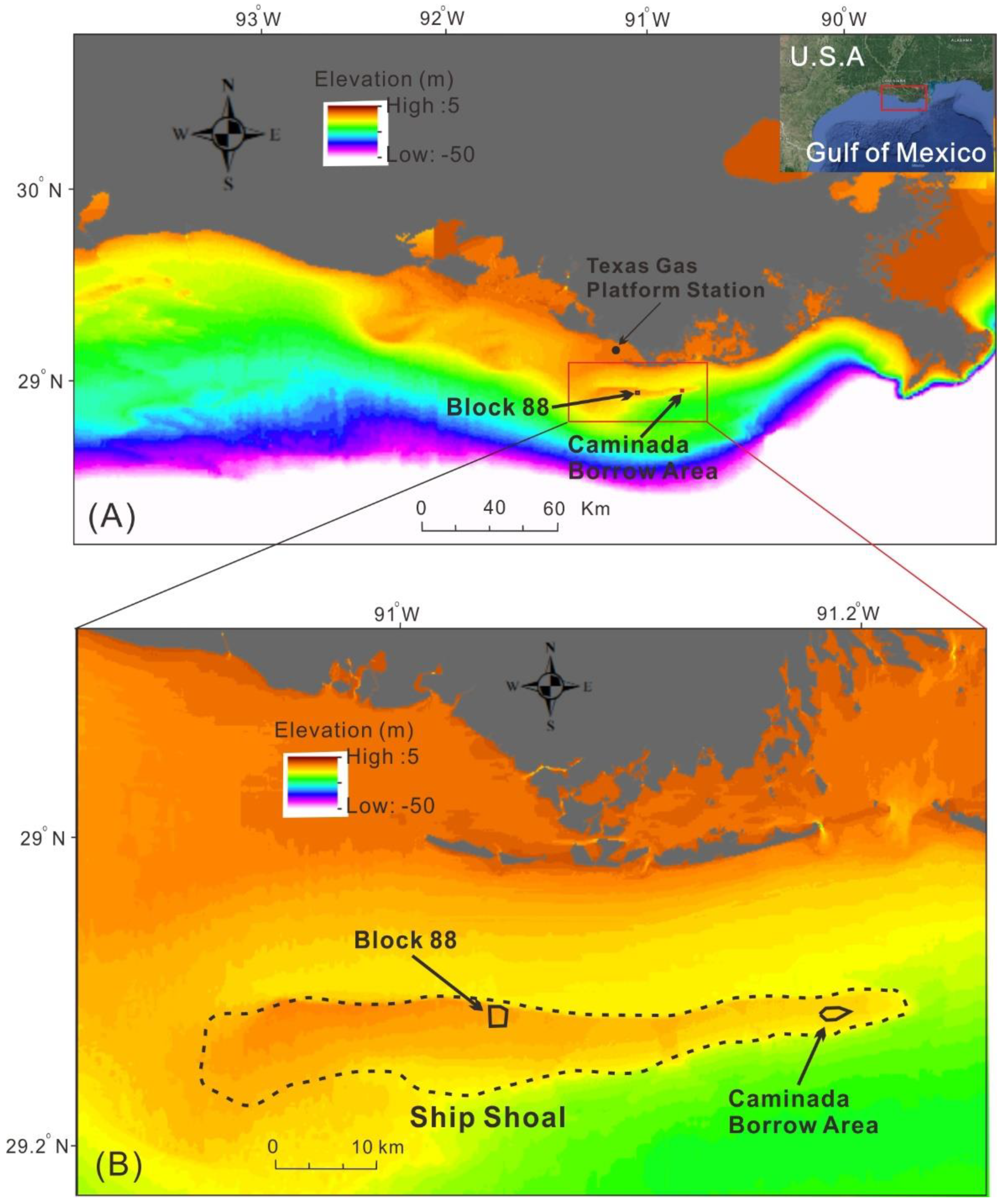
The Caminada Headland is a Gulf of Mexico shoreline that spans from Belle Pass on the west to Caminada Pass on the east, which is a distance of 21.4 km (Figure 2). The Caminada Headland Beach and Dune Restoration Projects were the first ones to use sand resources from the Ship Shoal area for barrier island restoration; these also comprised the costliest restoration effort, and the longest beach and dune restoration project in Louisiana to date [5]. The restoration of the Caminada Headland was comprised of two increments: Increment I (BA-45) and Increment II (BA-143). The Increment I Project (in 2014) was the first to utilize the sand resources from Ship Shoal. Subsequently, the Increment II Project (in 2016) for Caminada Headland and the Caillou Lake Headland Restoration ventured into the nearshore continental shelf for sediment resources. The area of the Caminada dredge pit (hereafter abbreviated as ‘Caminada’) is approximately 6.3 km2 (1.8 km × 3.5 km), and a total volume of 9.07 million m3 of sediment was dredged. Post-dredging volumetric analysis indicates that Caminada is presently infilling at an average rate of 0.15 m/year, or 27,480 m3/year [21].

3. Methods

3.1. Primary and Secondary Data

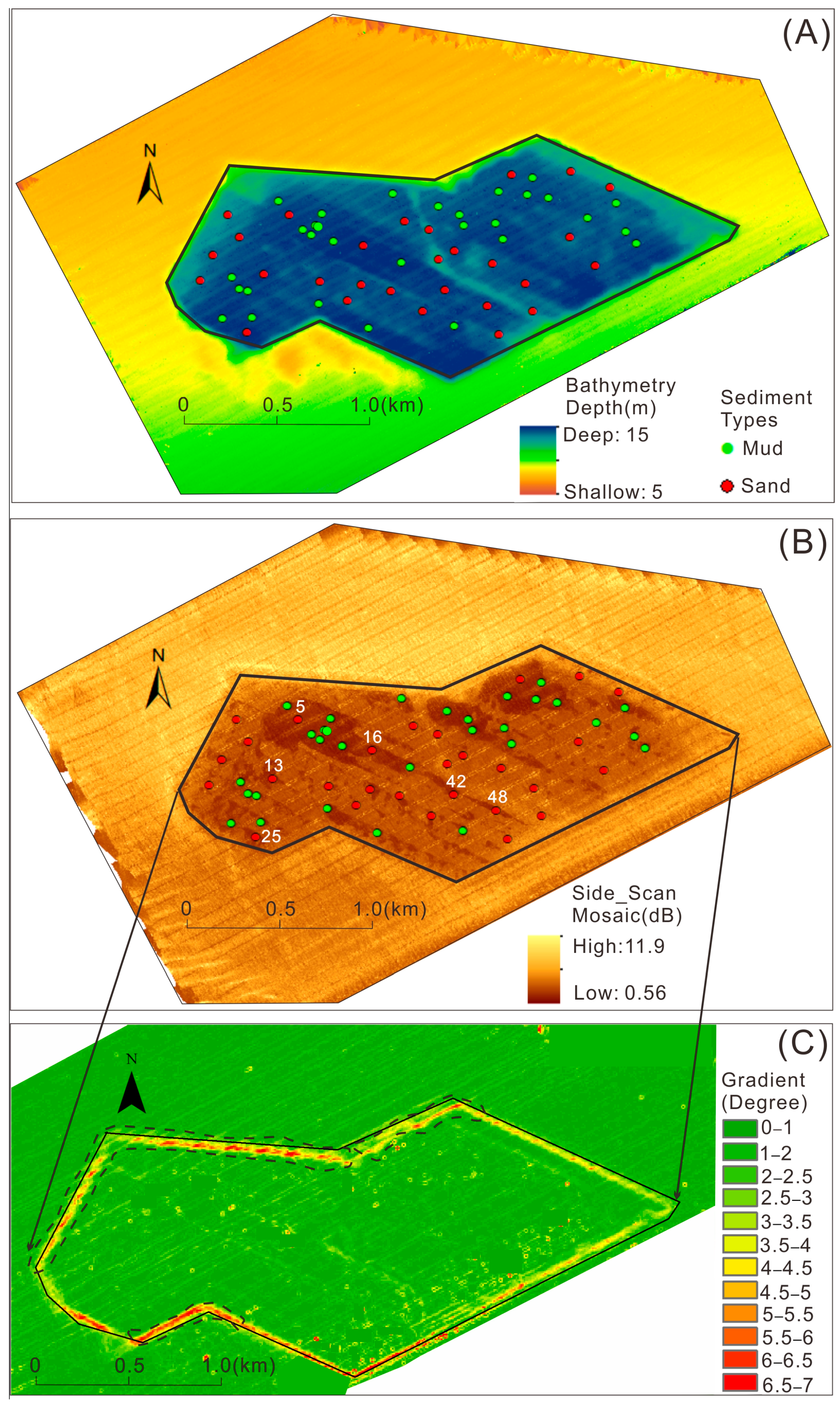
Bathymetric and side-scan sonar data were used to quantify the seafloor morphology and topography of the study area. Bathymetric data from a post-dredging survey in August 2018 were processed in CARIS HIPS and SIPS v.11.2 (Teledyne CARIS, Canada) (Figure 2A). The bathymetric data were referenced to an NOAA station at the Texas gas platform (Figure 1A), Caillou Bay, Louisiana (LA). Side-scan mosaics with backscatter values were first generated in CARIS and then exported into ArcMap (Figure 2B). Details of the processing and analysis of bathymetry and backscatter data can be found in Obelcz et al. [14] and Liu et al. [21].
The slope, aspect, curvature, and relative position of features and terrain variability were the derived secondary features of the bathymetry and backscatter datasets [36,37]. Some previous studies suggested a range of secondary features that were possibly associated with substrate types from terrain analysis, which includes the bathymetric position index (BPI), roughness, curvature, aspect, Moran’s I, and Sobel filter [28,29,30]. BPI is the vertical difference between a cell and the mean of the local neighborhood [36], which is deemed to be significant for sediment transport under the effect of waves and currents. This study used 20-m horizontal resolution as the cell size, which is hereafter defined as ‘BPI_20′. Roughness and rugosity are the derived features for terrain variability and refer to the difference between the minimum and maximum of cell and its eight neighbors, which is calculated on the basis of bathymetry and backscatter. Rugosity is a measure of small-scale variations of amplitude in the height of a surface, whereas roughness is the deviations in the direction of the normal vector of a real surface from its ideal form Wilson et al. [36]. In this study, all the derived secondary data were calculated in ArcGIS 10.0 via the BTM (Benthic Terrain Modeler) toolbox [38]. Since sediment samples in this study were collected in the relatively flat seabed with no obvious slope change (Figure 2C), the slope and aspect feature such as northness and eastness are subsequently removed from the derived features in this model. Then, BPI_20, Roughness_bathymetry (roughness derived from bathymetry), Roughness_backscatter (roughness derived from backscatter), and Rugosity_backscatter (rugosity derived from backscatter) were selected for further analysis, as described below (Table 1).

3.2. Surficial Sediment Data

Surficial sediment samples (n = 58) were collected using a clam-shell grab sampler in the bathymetric survey area in 2018. Grain size analysis was conducted using a Beckmann Coulter laser diffraction particle size analyzer (Model LS 13 320). A subsample from each grab (1 g) was digested with 30% hydrogen peroxide to remove any organic matter. More details of processing and analysis can be found in [21,22]. The sediment types were classified into two basic groups based on grain size analysis of the relative proportions of mud (median grain size d < 63 μm) and sand (63 μm < d < 2000 μm).

3.3. Classification Methods

Decision Tree [39,40,41] and Random Forest learning [41] were recently used in seabed mapping. Unlike parametric methods, tree-based methods do not have any parametric assumption on the data. Trees can automatically handle the mixed type of data (e.g., categorical and numeric variables) and missing values [42]. The recursive partition algorithm is a popular technique to construct a binary tree, in which each node can have at most two branches. At each splitting node, the tree algorithm finds the “optimal” splitting variable and location through exhaustive search. The “optimal” here means minimizing some predefined criterion, such as cross-entropy for classification and the sum of squared errors for regression. The splitting process is repeated recursively on the right and left branches derived from the previous split until some stopping criterion is met (e.g., the minimum sample size to split). Usually, a fully grown tree is highly complicated and overfits the data. In order to avoid overfitting, the algorithm “prunes” the overfitted tree by collapsing some internal splits and finds the optimal subtree that minimizes the cross-validation error [42]. In this study, the default setting was used to construct and prune the classification trees using the rpart package in R.
The Random Forest algorithm [43] is one of the most popular ensemble methods in data mining. The fundamental idea of Random Forest is to boost the prediction performance of a single tree by fitting multiple trees and combining their predictions. The Random Forest algorithm uses two ways to make the trees in the forest as diversified as possible. First, each tree is constructed using a random subset of the sample through bootstrapping (i.e., random sampling with replacement). Second, at each split, the optimal splitting variable is chosen from a random subset of variables. The observations not used to construct a tree are called out-of-bag samples. Instead of using cross-validation, the Random Forest algorithm uses the out-of-bag errors to estimate the predictive performance on new samples and stops growing more trees when the out-of-bag error converges. Additionally, regularized logistic regression was a popular classification method by adding a penalty term (e.g., lasso penalty) to the log-likelihood function [44], which can be used to pick out the most important features. The randomForest and glmnet packages with default settings were used in this study to run the Random Forest and regularized logistic regression models, respectively.
In this study, Random Forest, Decision Tree, and Regularized Logistic Regression with Lasso penalty (hereafter abbreviated as Logistic Lasso) were run using randomForest, rpart, and glmnet packages in R, respectively (Figure 3). The data were randomly split into training (80%) and test (20%) sets. The models were fitted using the training samples only, while the test samples were used to evaluate the models’ predictive performance. The results were based on a total of 250 random splits of the data. The accuracy rate and AUC (Area Under the Curve) score were used to evaluate the model performance [45]. Accuracy is defined as the proportion of samples that were correctly classified for the test set. AUC, which is based on the Receiver Operating Characteristic (ROC) curve, provides an aggregate measure of performance across all the possible classification thresholds. A model whose predictions are totally incorrect has an AUC of 0.0; one whose predictions are all correct has an AUC of 1.0. In our models, each sample contained (1) primary features: bathymetry (m) and backscatter data (dB), and (2) derived secondary features: BPI_20, Roughness_bathymetry, Roughness_backscatter, and Rugosity_backscatter. Each classification method in this study was trained three times using different combinations of features: (1) all six features, (2) only primary features (bathymetry and backscatter), and (3) a subset of features chosen by the Random Forest algorithm.

4. Results

4.1. Grain Sizes

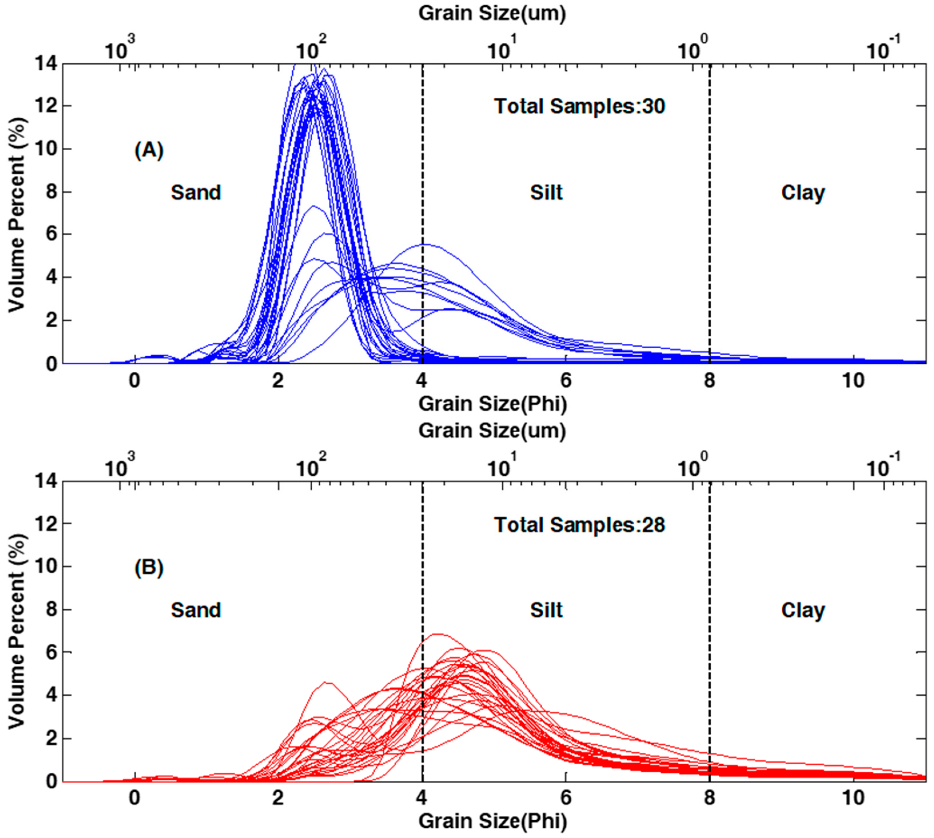
The grain size distributions of a total of 58 samples from Caminada pit are shown in Figure 3A,B. The majority of the 30 sandy samples within the pit contain about 90% sand and 10% silt, with modes around 100 µm (Figure 4A). However, there are a few sandy samples whose modes are near 63 µm. The grain sizes of the other 28 samples indicate the dominance of silt with modes around 15 µm (Figure 4B). On average, the sand, silt, and clay represent 21%, 75%, and 4%, respectively, with silt being the largest fraction.

4.2. Data Exploration

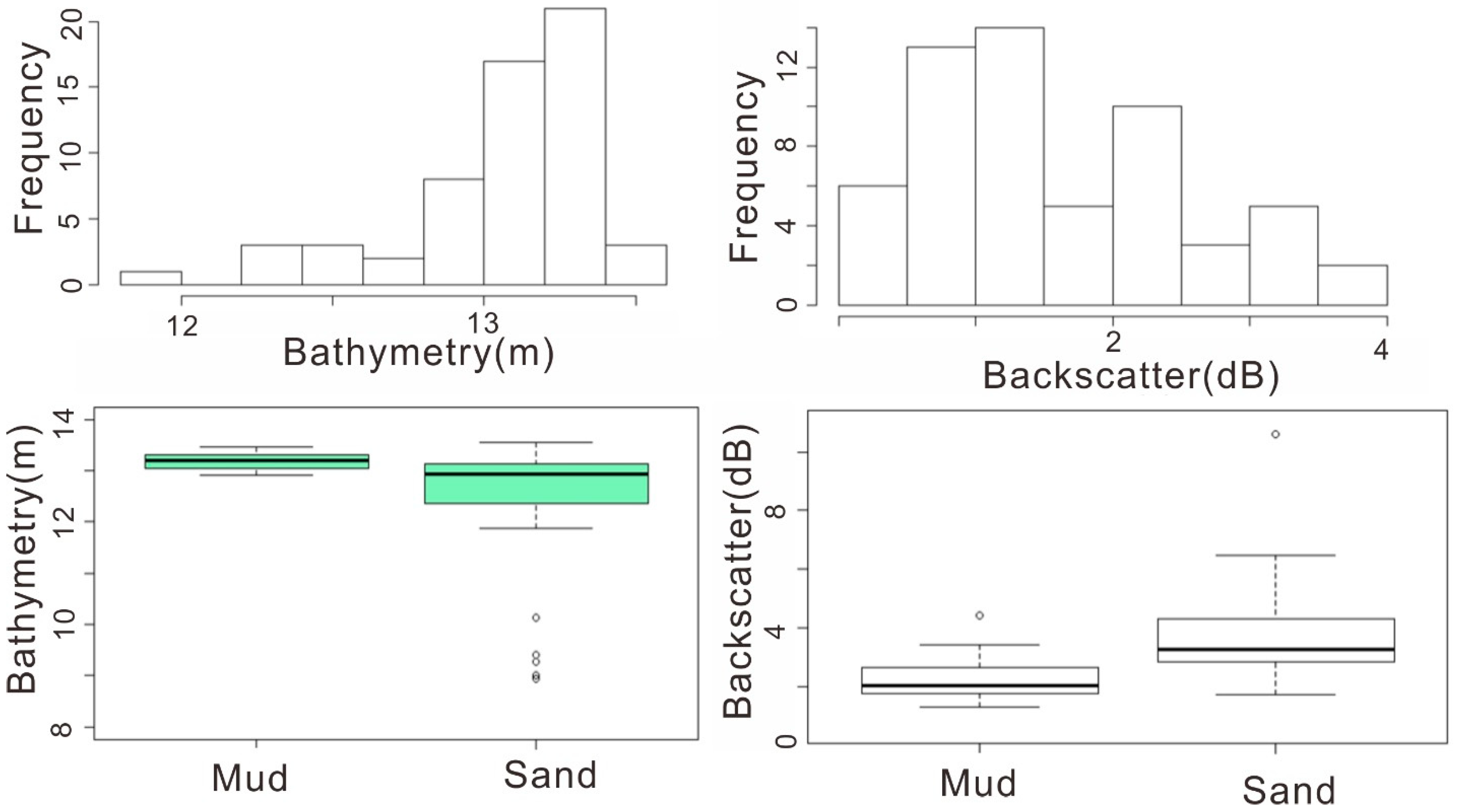
The training samples showed that the bathymetry of samples range from 9 m to 13.5 m, and most of the data are between 12.0–13.5 m (Figure 5A). The backscatter data revealed a sampling of values between 0–5 dB (Figure 5B), with the majority being in the 2–3 dB (Figure 5B). Further exploration of the sediment types of training data showed that, in general, coarser sediments were associated with higher backscatter and shallower water depths (Figure 5C,D).

4.3. Feature Selection

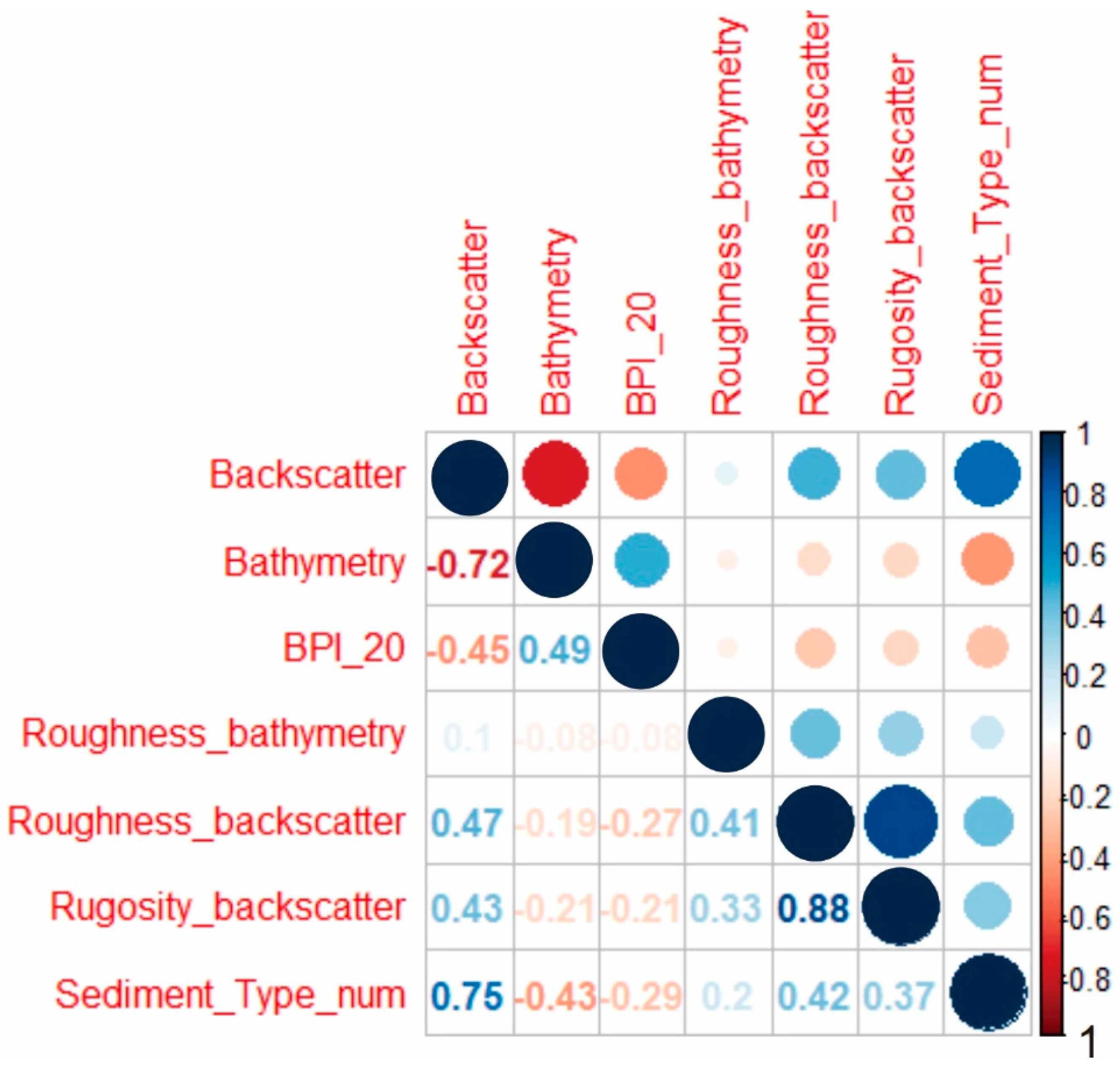
The correlation matrix shows that backscatter and bathymetry have a strong correlation with sediment types, and the absolute values are both greater than 0.43. Backscatter and all the corresponding derived features indicate a positive relationship with sediment types, whereas bathymetry and BPI_20 have a negative relationship with sediment types (Figure 6). It shows that a higher backscatter value with shallower water depth is prone to be classified as sand. The four derived features show autocorrelation with their original primary features. The Random Forest method was applied 10 times to calculate the variable importance (Table 2). The results indicate that backscatter, roughness_bathymetry, and rugosity_backscatter bathymetry were the most significant features that were included in the model with a subset of features.

4.4. Model Performance

Table 3 summarizes the test set performance for nine models (the combination of three sets of features and three classification methods) based on 250 random splits of the data. The number refers to three types of models with different input features used in the model. In set 1, all the features were used; in set 2, only the primary features (bathymetry and backscatter) were used; in set 3, a subset of four features chosen by the Random Forest algorithm discussed above was used. For example, DT1 stands for the Decision Tree model using all the features.
As we discussed above, each model was trained by 250 randomly split datasets, and then the average accuracy and standard deviation were recorded in Table 2. In terms of the first-type models, Classification Tree has the best performance with an accuracy of 0.84. However, the AUC only reaches 0.85, which is the smallest among all these three models. Likewise, the classification power increases when the model is only trained with the two primary features, which are the second-type models. The accuracy of the Logit_Lasso models increases from 0.83 to 0.84. Random Forest_2 has the best performance with the accuracy of 0.85 and AUC of 0.92. The best model of all the 12 is the Random Forest_3, which is trained by only four selected features, and reaches the accuracy of 0.90 and AUC of 0.95. Additionally, Decision Tree and Logistic Lasso classification take the longest time to run among all the 12 models.

5. Discussion

5.1. Model Evaluation and Comparison with Previous Studies

Previous studies show that the slope, aspect, curvature, and relative position of features and terrain variability were the four different geomorphological relevance in marine-based studies (Table 4) [37,39]. Slope can be used to evaluate the stability of sediments deposition/acceleration and erosion/movement, which are applied to calculate the basic slope (steepest) and directional slope [46,47,48,49,50,51]. Orientation is related to the direction of dominant geomorphic processes and the orientation of the seabed, i.e., which direction it is facing [52]. Aspect, Northness, and Eastness are the three terrain attributes of orientation [36]. Northness equals the cosine of the aspect, which is the direction of the steepest slope measured in clockwise degrees from north, and eastness refers to the sine of the aspect [53]. Curvature is useful in the classification of landforms, such as flow and the channeling of sediments/currents [51]. Previous studies used Mean Curvature [50], Profile Curvature [51,54], Plan Curvature [55], and BPI [56,57] to calculate terrain attributes of curvature. Lastly, the terrain variability and structures that are present reflect dominant geomorphic processes, which contains Rugosity [58], Vector Ruggedness [59], Bathymetric Roughness [36], Relative Relief [60], and Fractal Dimension [36]. In terms of our model, bathymetry and backscatter were identified as two important features in the model. Our results indicated that bathymetry roughness and backscatter roughness were two important secondary features, which is in line with multiple previous studies [27,28,30]. The BPI was not selected as a significant feature, which was possibly due to the relatively coarse cell size of 20 m when compared with the area of the seabed sampled by the grabs. Additionally, this study limited the number and types of input features in order to keep the model simulations manageable. A decision was made to limit the secondary features to those that were easily derived with standard GIS software to make this study comparable with others. Also, the slope and aspect of the seabed did not change dramatically inside the Caminada dredge pit, and thus northness and eastness were not used.
Supervised machine learning techniques that have been applied to seafloor mapping include Maximum Likelihood Estimation [60,61], k-Nearest Neighbor [62], Decision Trees [41,63], Random Forest [64], Artificial Neural Networks [64,65], and Support Vector Machines [61,65]. Many choices of supervised classification methods make it difficult to select the most appropriate method for a specific study site [28]. Brown et al. [66] classified the side-scan sonar mosaics into three groups and predicted the seabed surface characteristics of observed biological habitats via an unsupervised classification procedure in the United Kingdom with the water depth between 10–60 m. They also found there was a low-to-moderate correlation between the side-scan backscatter and particle size. Blondel et al. [31] applied the unsupervised classification of the k-means method to a textural analysis of Stanton Banks on Northern Ireland continental shelf with water depths varying from 120 to 160 m, and detected different types of seafloor based on multi-beam sonar imagery. Diesing et al. [27] compared different approaches including manual interpretation, geostatistics, object-based image analysis, and machine learning to test the accuracy of acoustic data interpretation in the western North Sea off the Scottish coast of the United Kingdom based on bathymetry, backscatter, as well as seabed samples in the water depth shallower than 100 m. They found that overall thematic classification accuracy was acceptable, but the difference among statistical methods was not significant. ML methods were also used to compare different supervised or unsupervised classification methods for the prediction of a marine benthic habitat using multi-beam echosounder and grain-size data [28]. Liu et al. [65] applied Decision Tree, Random Forest, Neural Network, and SVM to predict substrate types based on multi-beam sonar imagery in Busszard bay, Massachusetts. They found that Neural Network was a good option classifying sediment types of seafloor with complicated features. In terms of our four ML methods, the Random Forest method achieved the highest accuracy scores, performing significantly better than all the other model runs (Table 1). In terms of three combinations of input features, RF3 had the best classification power with an accuracy rate of 0.9. RF2 included only two primary features, but was not as good as RF3, which indicated bathymetry and backscatter data that contained partial information to classify the sediment types. Conversely, RF1 performed worse than all the other model runs according to the accuracy rates, indicating that the performance of all the features suffered due to the presence of some irrelevant features.
This study focused solely on the prediction performance of the classifiers, but did not focus on the tuning and training stages for the classifiers. In general, Random Forest and Logistic Lasso are computationally expensive algorithms compared to Decision Tree, since Random Forest is an ensemble of hundreds of trees, and Logistic Lasso requires choosing the tuning parameter through cross-validation. Additionally, this study focused solely on the classification approach to identify sediment types. Regression methods would be another path to reach a good prediction of variables.

5.2. Limitations and Future Work

After evaluating the models, some limitations of our work should be recognized. Firstly, the input features were aggregated to a particular spatial resolution. These were limited by sampling equipment (multi-beam sampling density) and more significantly, the computing power available for processing the data. The bathymetric and backscatter data were gridded to resolutions of 1 m and 10 m, respectively. However, the variations of sediment types within an area of 6300 m2 of the Caminada pit seafloor were not at the same scale as the bathymetric and backscatter grids. Future work should investigate the impacts of varying gridding cell sizes when the predictor variables have a coarser resolution than the sampling data.
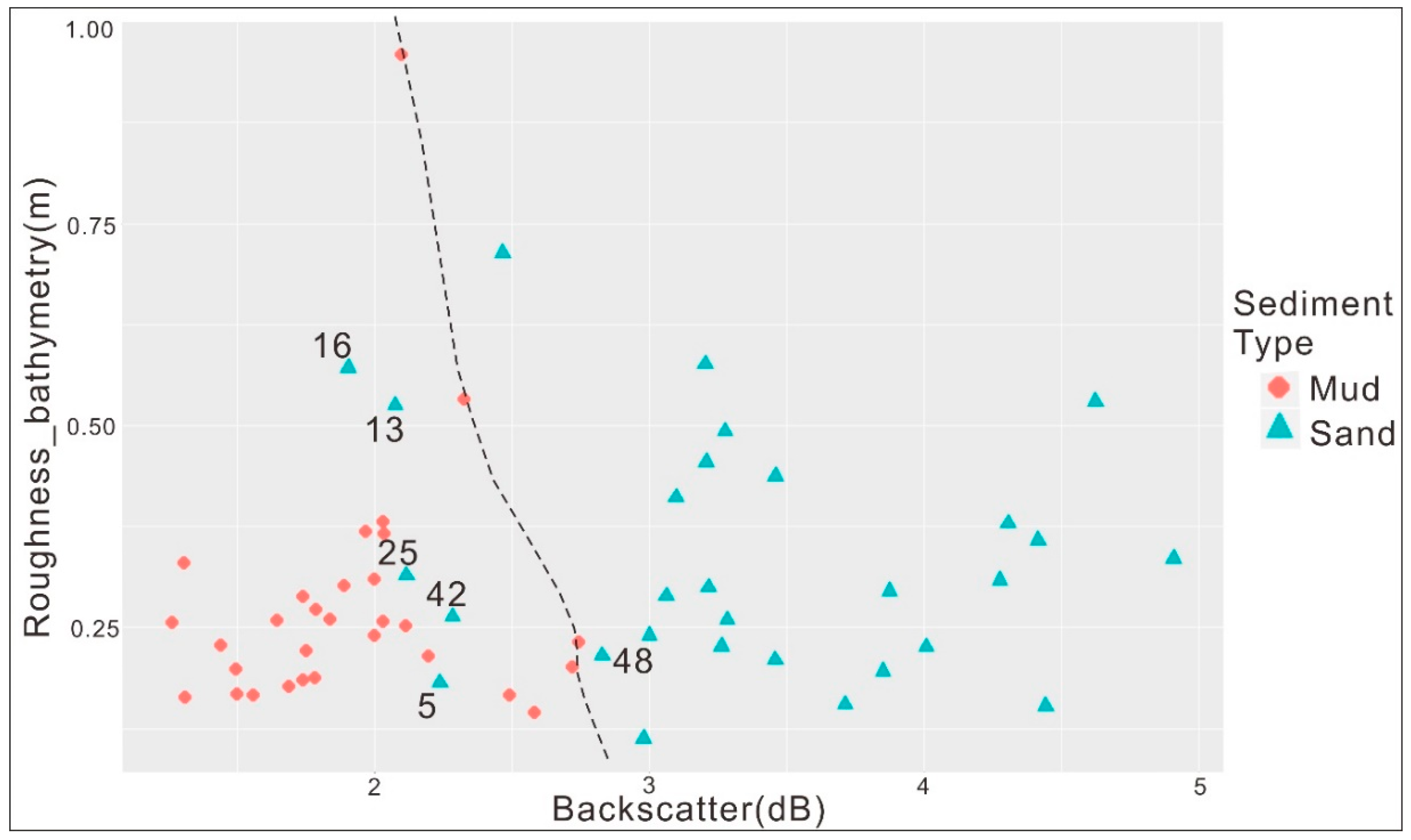
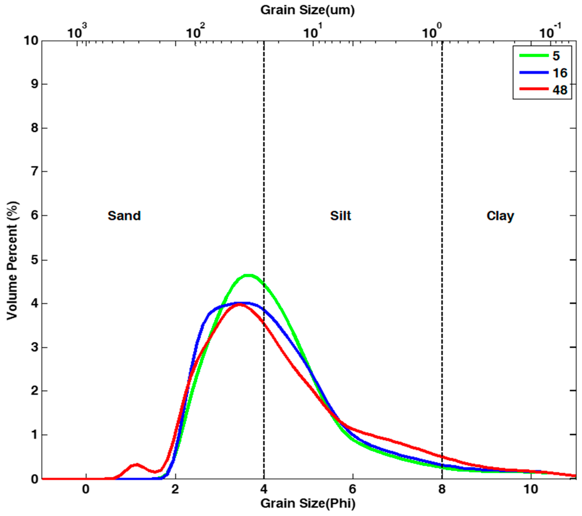
Secondly, the model was very capable of predicting dominantly sandy or muddy samples, but poor at predicting mud-sand mixture. Grain size analysis indicated the mixed sand and mud environment in the depression zones (Figure 2B and Figure 4). This study divided the sediment types into two types using 63 μm as the boundary. The mud–sand mixtures were challenging to predict, and they were also the misclassified ones. A partial dependence plot showed that six sandy samples existed near the classification boundary at 63 μm (Figure 7). Samples 5, 16, and 48 all have grain size modes near 63 μm (Figure 8), which was the blind zone of the model for classification. It also showed only sandy samples appeared across the classification boundary, which indicated that the model could better predict mud than sand (Figure 7).
Lastly, positional and sampling accuracy is a challenge in the field. In order to save time, our sampling boat was not anchored in the field. All 58 samples were collected in one day to save cost, and multiple trials were performed in some sandy sites in which it was hard to penetrate using a clam-shell grab sampler. Strong currents kept moving the boat when sediment samples were collected. It takes 3–5 min to collect one sample using the sampler, but the planned and actual sampling locations can be different. Also, strong currents caused some tilting of the winch cable attached to the grab sampler, leading to some coordinate differences between GPS on top of the boat and actual sampling locations on the pit bottom. Even a small difference between the planned and actual locations of sediment samples can be significant in Caminada pit, because of the mic-topography and patchy sediment distribution (Figure 4). A partial importance plot shows that samples 13, 25, and 42 are near the classification boundary (Figure 7). However, these three sandy samples exist in the depression zone (Figure 2B). According to the Random Forest model, these samples should contain high backscatter value, which is predicted as mud. The positional error of these three samples is likely the possible reason for the misclassification.

5.3. Implication to Coastal Restoration

It was reported that the majority of Caminada pit infilling is mainly derived from far-field muddy sediments either from the Mississippi River or Atchafalaya River or inner shelf sediments transported by currents and waves [17,21]. Caminada pit is in a unique depositional environment in which the existing sandy sediments are mixed with bypassing mud. Fine-grained bypassing muddy sediments were found inside Caminada and not considered as reusable resources. The change from sandy to muddy (or even mixed) substrate on Ship Shoal may greatly influence the activities of benthic communities. The deposition and redistribution of muddy inside Caminada would not allow the reuse of infilling sediment for future barrier island restoration. More time series geophysical, hydrodynamic, and sediment data are needed for post-construction management and monitoring in SSBA to evaluate whether the dredging activities in SSBA are cost-effective and sustainable [8,67].
Sandy shoals such as Tiger Shoal, Trinity Shoal, and Sabine Bank, ebb tidal deltas such Barataria Pass, and paleochannels in the Louisianan coastal zone all can potentially have mixed texture environments, similar to the Caminada pit. Block 88 in Ship Shoal was dredged recently in spring 2018 (Figure 1B), and had a depositional environment similar to the Caminada pit. Future dredging areas in coastal Louisianan zones will be focused on the sandy shoals and paleochannels, which are a sandy environment with possible mud trapping, and our model can be used for sediment identification in such an environment. Furthermore, the dredging pits in East and Gulf Coasts have a similar issue of the muddy sediment infilling in sandy pits. Manasquan Inlet (New Jersey), Mobile Bay (Alabama), and Mobile Quter mound (Alabama) were predicted to exist for more than 100 years due to less sediment supply and transport [3]. Our model provides a new method to predict the change of mixed sediments (mud and sand) distribution inside sandy dredge pits for post-construction management. However, this model may not be applied to a homogenous substrate such as the muddy bay areas where sediment is more uniform; similarly, this model probably would not perform well when new sand fills in a sandy pit. Hard bottoms and oyster reefs are substrate types differing with sand and mud. Our model did not include these substrate types due to lack of such substrate in Caminada pit, but our method can be used to predict a variety of contrasting seabed substrate types in future research.
Additionally, dredge pits in Ship Shoal are in inner-shelf shoals offshore Louisiana, where dredging and transporting sediment from offshore is expensive as nearshore sediment sources are being explored and depleted [6]. Our model provides a cost-saving method to evaluate the seafloor sediments in a sand–mud mixed environment. Our results show that backscatter is the single most important feature to predict sediment types (Table 2). When the budget is limited, only collecting backscatter data will be acceptable and cost-effective because of its powerful prediction capability. In other words, after establishing a reliable ML model for dredge pits, sediment samples and multi-beam data can be collected much less frequently than side-scan data. When a monitoring plan is developed, sediment and multi-beam data may be collected once every year, or even every other year, whereas side-scan data can be collected seasonally. Synthesizing observation with modeling would eventually yield the best results for sandy resource management. Our results can also be used to better understand the impacts on biological communities by direct defaunation due to sand excavation and mud accumulation in topographic lows. This study can increase the government’s decision-making ability regarding safety and protecting environmental and cultural resources.

6. Conclusions

The sand volume of Caminada dredge pit in Ship Shoal is one of the largest on the United States (USA) east and Gulf coasts. The integration of the bathymetric data, backscatter data, and sediment collection in 2018 enabled us to apply ML methods to identify the mud deposition and classify the seafloor sediment types in Caminada dredge pit on the continental shelf offshore Louisiana, USA.
(1)
Grain size analysis of the 58 sediment samples inside the dredge pit shows that mud is prone to deposit in trough zones with lower backscatter values, while sand is likely to appear on the flat seabed with higher backscatter values.
(2)
The variable importance analysis indicates that backscatter, roughness_bathymetry, rugosity_backscatter, and bathymetry (from high to low) are the four most significant features to classify sediment types. A Random Forest model with these four selected features has the best classification power with the accuracy rate of 0.9 to predict the sediment types inside the dredge pit.
(3)
The particular spatial resolution between multi-beam density and the availability of sediment type, a simple mud–sand classification method, and the positional accuracy of the sediment samples collected in the field are the three possible factors that likely lead to differences between the planned and actual locations of sediment samples.
(4)
The deposition and redistribution of mud inside the Caminada pit make it unusable for barrier island restoration, but our model provides a new and efficient method to predict the time-series change of sediments (mud and sand) distribution inside the Caminada pit for post-construction management.

Author Contributions

Conceptualization, H.L. and K.X.; methodology, H.L., K.X. and B.L.; software, Y.H. and G.L.; validation, H.L. and B.L.; Formal analysis, H.L. and Y.H.; investigation, K.X. and B.L.; resources, Y.H.; data curation, K.X. and G.L.; writing—original draft preparation, H.L.; writing—review and editing, K.X. and B.L.; visualization, B.L. and Y.H.; supervision, K.X.; project administration, K.X.; funding acquisition, K.X.

Funding

Funding for this study was provided by the U.S. Department of the Interior, Bureau of Ocean Energy Management, Coastal Marine Institute, Washington DC, under Cooperative Agreement Number M16AC00018.

Acknowledgments

We are thankful to the Field Support Group of Coastal Studies Institute, Robert Bales and Kelli Moran from Sediment Dynamics Lab, Carol Wilson’ group and the editing help from Nancy Rabalais from Louisiana State University. The first author’s Ph.D. program was founded by Economic Development Assistantship from the Graduate School of Louisiana State University.

Conflicts of Interest

The authors declare no conflict of interest.

References

  1. Syvitski, J.P.; Kettner, A.J.; Overeem, I.; Hutton, E.W.; Hannon, M.T.; Brakenridge, G.R.; Day, J.; Vörösmarty, C.; Saito, Y.; Giosan, L. Sinking deltas due to human activities. Nat. Geosci. 2009, 2, 681. [Google Scholar] [CrossRef]
  2. Vörösmarty, C.J.; Syvitski, J.; Day, J.; De Sherbinin, A.; Giosan, L.; Paola, C. Battling to save the world’s river deltas. Bull. At. Sci. 2009, 65, 31–43. [Google Scholar] [CrossRef]
  3. Byrnes, M.R.; Hammer, R.M.; Thibaut, T.D.; Snyder, D.B. Physical and biological effects of sand mining offshore Alabama, USA. J. Coast. Res. 2004, 20, 6–24. [Google Scholar] [CrossRef]
  4. Kennedy, A.B.; Slatton, K.C.; Starek, M.; Kampa, K.; Cho, H.-C. Hurricane response of nearshore borrow pits from airborne bathymetric lidar. J. Waterw. Port Coast. Ocean Eng. 2009, 136, 46–58. [Google Scholar] [CrossRef]
  5. CEC; CECI. NRDA Caminada Headland Beach and Dune Restoration, Increment II (BA-143) Completion Report; Prepared for Coastal Protection and Restoration Authority: Baton Rouge, LA, USA, 2017. [Google Scholar]
  6. Syed Khalil, A.F.; Richard, C. Raynie, Sediment management for sustainable ecosystem restoration of coastal Louisiana. Shore Beach 2018, 86, 17–27. [Google Scholar]
  7. Allison, M.A.; Ramirez, M.T.; Meselhe, E.A. Diversion of Mississippi River water downstream of New Orleans, Louisiana, USA to maximize sediment capture and ameliorate coastal land loss. Water Resour. Manag. 2014, 28, 4113–4126. [Google Scholar] [CrossRef]
  8. Stone, G.; Condrey, R.; Fleeger, J.; Khalil, S.; Kobashi, D.; Jose, F.; Evers, E.; Dubois, S.; Liu, B.; Arndt, S. Environmental Investigation of Long-Term Use of Ship Shoal Sand Resources for Large Scale Beach and Coastal Restoration in Louisiana; OCS Study MMS; US Dept. of the Interior, Minerals Management Service, Gulf of Mexico OCS Region: New Orleans, LA, USA, 2009; Volume 24, p. 278.
  9. Hanley, M.; Hoggart, S.; Simmonds, D.; Bichot, A.; Colangelo, M.; Bozzeda, F.; Heurtefeux, H.; Ondiviela, B.; Ostrowski, R.; Recio, M. Shifting sands? Coastal protection by sand banks, beaches and dunes. Coast. Eng. 2014, 87, 136–146. [Google Scholar] [CrossRef]
  10. Jonah, F.E.; Adjei-Boateng, D.; Agbo, N.W.; Mensah, E.A.; Edziyie, R.E. Assessment of sand and stone mining along the coastline of Cape Coast, Ghana. Ann. GIS 2015, 21, 223–231. [Google Scholar] [CrossRef]
  11. Brown, J.M.; Amoudry, L.O.; Souza, A.J.; Rees, J. Fate and pathways of dredged estuarine sediment spoil in response to variable sediment size and baroclinic coastal circulation. J. Environ. Manag. 2015, 149, 209–221. [Google Scholar] [CrossRef] [Green Version]
  12. Rangel-Buitrago, N.G.; Anfuso, G.; Williams, A.T. Coastal erosion along the Caribbean coast of Colombia: Magnitudes, causes and management. Ocean. Coast. Manag. 2015, 114, 129–144. [Google Scholar] [CrossRef]
  13. Dubois, S.; Gelpi, C.G.; Condrey, R.E.; Grippo, M.A.; Fleeger, J.W. Diversity and composition of macrobenthic community associated with sandy shoals of the Louisiana continental shelf. Biodivers. Conserv. 2009, 18, 3759–3784. [Google Scholar] [CrossRef]
  14. Obelcz, J.; Xu, K.; Bentley, S.J.; O’Connor, M.; Miner, M.D. Mud-capped dredge pits: An experiment of opportunity for characterizing cohesive sediment transport and slope stability in the northern Gulf of Mexico. Estuar. Coast. Shelf Sci. 2018, 208, 161–169. [Google Scholar] [CrossRef]
  15. Wang, J.; Xu, K.; Li, C.; Obelcz, J. Forces Driving the Morphological Evolution of a Mud-Capped Dredge Pit, Northern Gulf of Mexico. Water 2018, 10, 1001. [Google Scholar] [CrossRef]
  16. Liu, H.; Xu, K.; Bentley, S.; Li, C.; Miner, M.; Wilson, C.; Xue, Z. Sediment Transport and Slope Stability of Ship Shoal Borrow Areas for Coastal Restoration of Louisiana. In Proceedings of the AGU Fall Meeting Abstracts, New Orleans, LA, USA, 11–15 December 2017. [Google Scholar]
  17. Xue, Z.; Wilson, C.; Bentley, S.J.; Xu, K.; Liu, H.; Li, C.; Miner, M.D. Quantifying Sediment Characteristics and Infilling Rate within a Ship Shoal Dredge Borrow Area, Offshore Louisiana. In Proceedings of the AGU Fall Meeting Abstracts, New Orleans, LA, USA, 11–15 December 2017. [Google Scholar]
  18. Pearce, D.W. Valuing the Environment: Past Practice, Future Prospect; Citeseerx, Pennsylvania State University, USA: Centre County, PA, USA, 1994. [Google Scholar]
  19. Nairn, R.; Johnson, J.A.; Hardin, D.; Michel, J. A biological and physical monitoring program to evaluate long-term impacts from sand dredging operations in the United States outer continental shelf. J. Coast. Res. 2004, 20, 126–137. [Google Scholar] [CrossRef]
  20. Munnelly, R.T.; Reeves, D.B.; Chesney, E.J.; Baltz, D.M. Summertime hydrography of the nearshore Louisiana Continental Shelf: Effects of riverine outflow, shelf morphology, and the presence of sand shoals on water quality. Cont. Shelf Res. 2019, 179, 18–36. [Google Scholar] [CrossRef]
  21. Liu, H.; Xu, K.; Bentley, S.; Wilson, C.; Xue, Z.; Miner, M. Sediment transport and geomorphologic response in multiple dredge pits near Ship Shoal of coastal Louisiana. In Proceedings of the AGU Fall Meeting Abstracts, Washington, DC, USA, 10–14 December 2018. [Google Scholar]
  22. Xu, K.; Corbett, D.; Walsh, J.; Young, D.; Briggs, K.; Cartwright, G.; Friedrichs, C.; Harris, C.; Mickey, R.; Mitra, S. Seabed erodibility variations on the Louisiana continental shelf before and after the 2011 Mississippi River flood. Estuar. Coast. Shelf Sci. 2014, 149, 283–293. [Google Scholar] [CrossRef]
  23. Denny, J.; Baldwin, W.; Schwab, W.; Gayes, P.; Morton, R.; Driscoll, N. Morphology and Texture of Modern Sediments on the Inner Shelf of South Carolina’s Long Bay from Little River Inlet to Winyah Bay; No. 2331-1258; US Geological Survey: Reston, VA, USA, 2007.
  24. Freeman, A.M.; Roberts, H.H.; Banks, P.D. Hurricane impact analysis of a Louisiana shallow coastal bay bottom and its shallow subsurface geology. Gulf Coast Assoc. Geol. Soc. Trans. 2007, 255–267. [Google Scholar]
  25. Karpatne, A.; Ebert-Uphoff, I.; Ravela, S.; Babaie, H.A.; Kumar, V. Machine learning for the geosciences: Challenges and opportunities. IEEE Trans. Knowl. Data Eng. 2018. [Google Scholar] [CrossRef]
  26. Reichstein, M.; Camps-Valls, G.; Stevens, B.; Jung, M.; Denzler, J.; Carvalhais, N. Deep learning and process understanding for data-driven Earth system science. Nature 2019, 566, 195. [Google Scholar] [CrossRef] [PubMed]
  27. Diesing, M.; Green, S.L.; Stephens, D.; Lark, R.M.; Stewart, H.A.; Dove, D. Mapping seabed sediments: Comparison of manual, geostatistical, object-based image analysis and machine learning approaches. Cont. Shelf Res. 2014, 84, 107–119. [Google Scholar] [CrossRef] [Green Version]
  28. Stephens, D.; Diesing, M. A comparison of supervised classification methods for the prediction of substrate type using multibeam acoustic and legacy grain-size data. PLoS ONE 2014, 9, e93950. [Google Scholar] [CrossRef] [PubMed]
  29. Valentine, A.; Kalnins, L. An introduction to learning algorithms and potential applications in geomorphometry and earth surface dynamics. Earth Surf. Dyn. 2016, 4, 445–460. [Google Scholar] [CrossRef]
  30. Lacharité, M.; Brown, C.J.; Gazzola, V. Multisource multibeam backscatter data: Developing a strategy for the production of benthic habitat maps using semi-automated seafloor classification methods. Mar. Geophys. Res. 2018, 39, 307–322. [Google Scholar] [CrossRef]
  31. Blondel, P.; Sichi, O.G. Textural analyses of multibeam sonar imagery from Stanton Banks, Northern Ireland continental shelf. Appl. Acoust. 2009, 70, 1288–1297. [Google Scholar] [CrossRef]
  32. Penland, S.; Connor, P.F., Jr.; Beall, A.; Fearnley, S.; Williams, S.J. Changes in Louisiana’s shoreline: 1855–2002. J. Coast. Res. 2005, 21, 7–39. [Google Scholar]
  33. Drucker, B.S.; Waskes, W.; Byrnes, M.R. The US minerals management service outer continental shelf sand and gravel program: Environmental studies to assess the potential effects of offshore dredging operations in federal waters. J. Coast. Res. 2004, 20, 1–5. [Google Scholar] [CrossRef]
  34. Khalil, S.M.; Finkl, C.W.; Andrews, J.; Knotts, C.P. Restoration-quality sand from Ship Shoal, Louisiana: Geotechnical investigation for sand on a drowned barrier island. In Proceedings of the Coastal Sediments’ 07, New Orleans, Louisiana, 13–17 May 2007; Volume 7, pp. 685–698. [Google Scholar]
  35. Williams, S.J.; Flocks, J.; Jenkins, C.; Khalil, S.; Moya, J. Offshore sediment character and sand resource assessment of the northern Gulf of Mexico, Florida to Texas. J. Coast. Res. 2012, 30–44. [Google Scholar] [CrossRef]
  36. Wilson, M.F.; O’Connell, B.; Brown, C.; Guinan, J.C.; Grehan, A.J. Multiscale terrain analysis of multibeam bathymetry data for habitat mapping on the continental slope. Mar. Geod. 2007, 30, 3–35. [Google Scholar] [CrossRef]
  37. Lecours, V.; Dolan, M.F.; Micallef, A.; Lucieer, V.L. A review of marine geomorphometry, the quantitative study of the seafloor. Hydrol. Earth Syst. Sci. 2016, 20, 3207. [Google Scholar] [CrossRef]
  38. Walbridge, S.; Slocum, N.; Pobuda, M.; Wright, D. Unified geomorphological analysis workflows with benthic terrain modeler. Geosciences 2018, 8, 94. [Google Scholar] [CrossRef]
  39. Buhl-Mortensen, P.; Dolan, M.; Buhl-Mortensen, L. Prediction of benthic biotopes on a Norwegian offshore bank using a combination of multivariate analysis and GIS classification. ICES J. Mar. Sci. 2009, 66, 2026–2032. [Google Scholar] [CrossRef]
  40. Gonzalez-Mirelis, G.; Lindegarth, M. Predicting the distribution of out-of-reach biotopes with decision trees in a Swedish marine protected area. Ecol. Appl. 2012, 22, 2248–2264. [Google Scholar] [CrossRef] [PubMed]
  41. Ierodiaconou, D.; Monk, J.; Rattray, A.; Laurenson, L.; Versace, V. Comparison of automated classification techniques for predicting benthic biological communities using hydroacoustics and video observations. Cont. Shelf Res. 2011, 31, S28–S38. [Google Scholar] [CrossRef]
  42. Atkinson, E.J.; Therneau, T.M. An Introduction to Recursive Partitioning Using the RPART Routines; Mayo Foundation: Rochester, NY, USA, 2000. [Google Scholar]
  43. Breiman, L. Bagging predictors. Mach. Learn. 1996, 24, 123–140. [Google Scholar] [CrossRef] [Green Version]
  44. Tibshirani, R. Regression shrinkage and selection via the lasso: A retrospective. J. R. Stat. Soc. Ser. B Stat. Methodol. 2011, 73, 273–282. [Google Scholar] [CrossRef]
  45. Huang, J.; Ling, C.X. Using AUC and accuracy in evaluating learning algorithms. IEEE Trans. Knowl. Data Eng. 2005, 17, 299–310. [Google Scholar] [CrossRef]
  46. Lundblad, E.R.; Wright, D.J.; Miller, J.; Larkin, E.M.; Rinehart, R.; Naar, D.F.; Donahue, B.T.; Anderson, S.M.; Battista, T. A benthic terrain classification scheme for American Samoa. Mar. Geod. 2006, 29, 89–111. [Google Scholar] [CrossRef]
  47. Lanier, A.; Romsos, C.; Goldfinger, C. Seafloor habitat mapping on the Oregon continental margin: A spatially nested GIS approach to mapping scale, mapping methods, and accuracy quantification. Mar. Geod. 2007, 30, 51–76. [Google Scholar] [CrossRef]
  48. Micallef, A.; Le Bas, T.P.; Huvenne, V.A.; Blondel, P.; Hühnerbach, V.; Deidun, A. A multi-method approach for benthic habitat mapping of shallow coastal areas with high-resolution multibeam data. Cont. Shelf Res. 2012, 39, 14–26. [Google Scholar] [CrossRef]
  49. Micallef, A.; Mountjoy, J.J.; Canals, M.; Lastras, G. Deep-seated bedrock landslides and submarine canyon evolution in an active tectonic margin: Cook Strait, New Zealand. In Submarine Mass Movements and Their Consequences; Springer: Berlin/Heidelberg, Germany, 2012; pp. 201–212. [Google Scholar]
  50. Dolan, M.F.; Lucieer, V.L. Variation and uncertainty in bathymetric slope calculations using geographic information systems. Mar. Geod. 2014, 37, 187–219. [Google Scholar] [CrossRef]
  51. Jenness, J.S. Calculating landscape surface area from digital elevation models. Wildl. Soc. Bull. 2004, 32, 829–840. [Google Scholar] [CrossRef]
  52. Galparsoro, I.; Borja, Á.; Bald, J.; Liria, P.; Chust, G. Predicting suitable habitat for the European lobster (Homarus gammarus), on the Basque continental shelf (Bay of Biscay), using Ecological-Niche Factor Analysis. Ecol. Model. 2009, 220, 556–567. [Google Scholar] [CrossRef]
  53. Monk, J.; Ierodiaconou, D.; Bellgrove, A.; Harvey, E.; Laurenson, L. Remotely sensed hydroacoustics and observation data for predicting fish habitat suitability. Cont. Shelf Res. 2011, 31, S17–S27. [Google Scholar] [CrossRef]
  54. Guinan, J.; Brown, C.; Dolan, M.F.; Grehan, A.J. Ecological niche modelling of the distribution of cold-water coral habitat using underwater remote sensing data. Ecol. Inform. 2009, 4, 83–92. [Google Scholar] [CrossRef]
  55. Ross, L.K.; Ross, R.E.; Stewart, H.A.; Howell, K.L. The influence of data resolution on predicted distribution and estimates of extent of current protection of three ‘listed’ deep-sea habitats. PLoS ONE 2015, 10, e0140061. [Google Scholar] [CrossRef] [PubMed]
  56. Monk, J.; Ierodiaconou, D.; Versace, V.L.; Bellgrove, A.; Harvey, E.; Rattray, A.; Laurenson, L.; Quinn, G.P. Habitat suitability for marine fishes using presence-only modelling and multibeam sonar. Mar. Ecol. Prog. Ser. 2010, 420, 157–174. [Google Scholar] [CrossRef] [Green Version]
  57. Pirtle, J.L.; Weber, T.C.; Wilson, C.D.; Rooper, C.N. Assessment of trawlable and untrawlable seafloor using multibeam-derived metrics. Methods Oceanogr. 2015, 12, 18–35. [Google Scholar] [CrossRef]
  58. Dunn, D.C.; Halpin, P.N. Rugosity-based regional modeling of hard-bottom habitat. Mar. Ecol. Prog. Ser. 2009, 377, 1–11. [Google Scholar] [CrossRef] [Green Version]
  59. Tempera, F.; Giacomello, E.; Mitchell, N.C.; Campos, A.S.; Henriques, A.B.; Bashmachnikov, I.; Martins, A.; Mendonça, A.; Morato, T.; Colaço, A. Mapping Condor seamount seafloor environment and associated biological assemblages (Azores, NE Atlantic). In Seafloor Geomorphology as Benthic Habitat; Elsevier: Amsterdam, The Netherlands, 2012; pp. 807–818. [Google Scholar]
  60. Elvenes, S. Landscape Mapping in MAREANO; NGU Report 2013.035; Geological Survey of Norway: Trondheim, Norway, 2013. [Google Scholar]
  61. Hasan, R.C.; Ierodiaconou, D.; Laurenson, L. Combining angular response classification and backscatter imagery segmentation for benthic biological habitat mapping. Estuar. Coast. Shelf Sci. 2012, 97, 1–9. [Google Scholar] [CrossRef] [Green Version]
  62. Lucieer, V.; Hill, N.A.; Barrett, N.S.; Nichol, S. Do marine substrates ‘look’ and ‘sound’ the same? Supervised classification of multibeam acoustic data using autonomous underwater vehicle images. Estuar. Coast. Shelf Sci. 2013, 117, 94–106. [Google Scholar] [CrossRef]
  63. Hasan, R.; Ierodiaconou, D.; Monk, J. Evaluation of four supervised learning methods for benthic habitat mapping using backscatter from multi-beam sonar. Remote Sens. 2012, 4, 3427–3443. [Google Scholar] [CrossRef]
  64. Marsh, I.; Brown, C. Neural network classification of multibeam backscatter and bathymetry data from Stanton Bank (Area IV). Appl. Acoust. 2009, 70, 1269–1276. [Google Scholar] [CrossRef]
  65. Liu, H.; Zheng, Z.; Wang, J.; He, S. A comparison of supervised classification methods for prediction and mapping of sediment types with multibeam bathymetry and backscatter data in Buzzards Bay, Massachusetts. In Proceedings of the AGU Fall Meeting Abstracts, Washington, DC, USA, 10–14 December 2018. [Google Scholar]
  66. Brown, C.J.; Collier, J.S. Mapping benthic habitat in regions of gradational substrata: An automated approach utilising geophysical, geological, and biological relationships. Estuar. Coast. Shelf Sci. 2008, 78, 203–214. [Google Scholar] [CrossRef]
  67. Xu, K.; Bargu, S.; Bentley, S.J.; Duplantis, B.; Li, C.; Maiti, K.; Miner, M.D.; White, J.R.; Wilson, C.; Xue, Z.G. Sediment Transport and Water Quality of a Dredge Pit on Louisiana Shelf for Coastal Restoration. In Proceedings of the AGU Fall Meeting Abstracts, Washington, DC, USA, 10–14 December 2018. [Google Scholar]
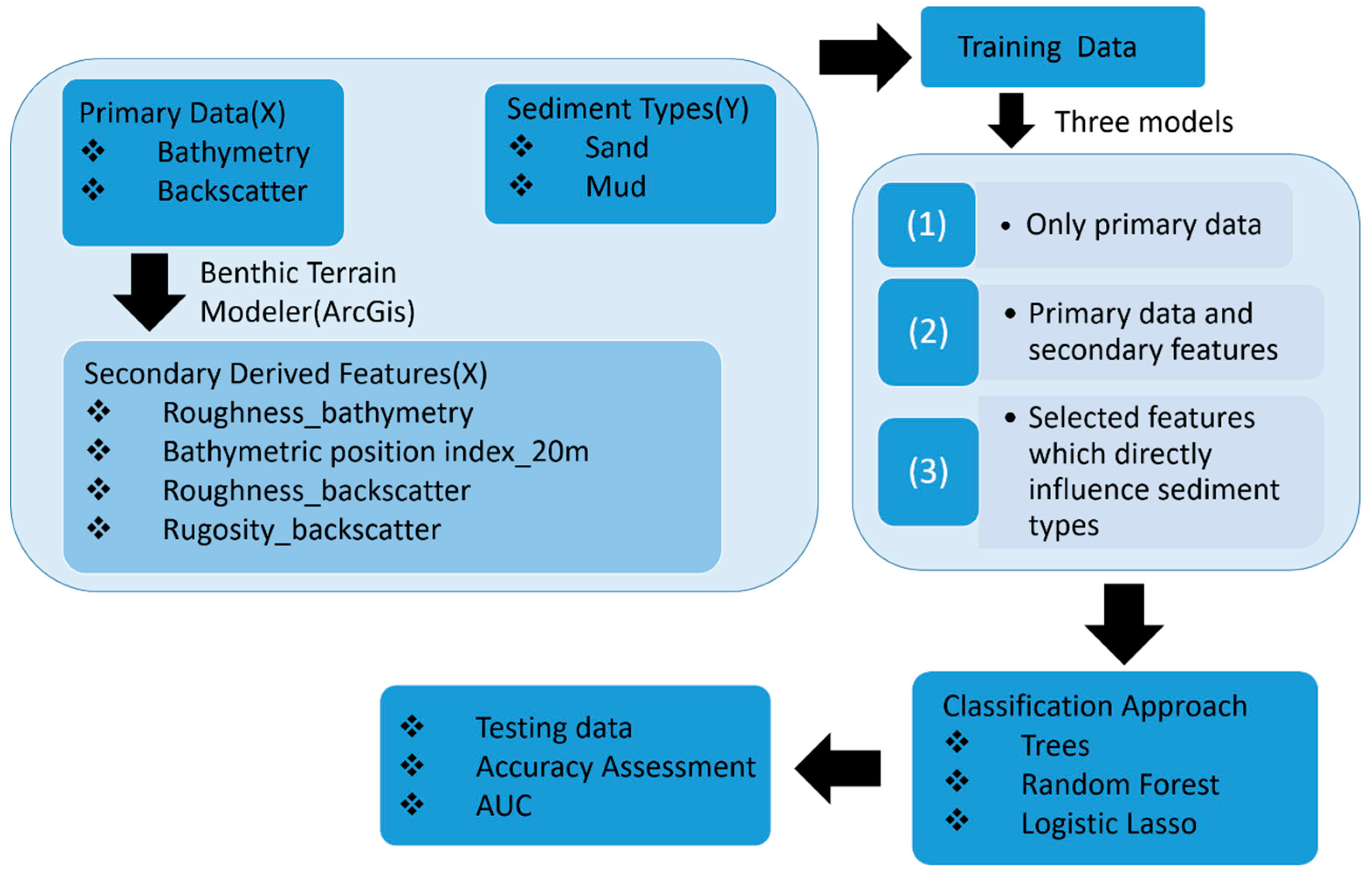
Figure 1. (A) A map showing the location of two sandy pits along the Louisiana shelf. The Texas gas platform station is the NOAA (National Oceanic and Atmospheric Administration) tide and current station (ID: 8763535) for tide and bathymetry correction. (B) Two borrow areas in Ship Shoal are Block 88 and Caminada. This study focuses on the Caminada dredge pit.
Water 11 01257 g001
Figure 2. (A) Bathymetry map in a survey from August 2018 with 1-m horizontal resolution. The depth value is positive with a unit of meter. (B) Side-scan map of Caminada pit in August 2018 with 10-m resolution. Note that the dark brown indicates the patchy mud with low backscatter values, while the bright yellow is associated with sandy sediment with high backscatter values. (C) Gradient map of the Caminada pit derived from August 2018 bathymetry. Green colors represent flatter surfaces, while red colors indicate steeper ones. The dotted polygons are steep pit walls.
Water 11 01257 g002
Figure 3. Flowchart of models which covers input features, machine learning (ML) methods, and validation methods.
Water 11 01257 g003
Figure 4. Grain size distributions of surficial sediment samples collected inside Caminada pit in August 2018 (see Figure 2B for grab sample locations). (A) Shows the grain size distribution of 30 sandy samples and (B) shows 28 muddy samples.
Water 11 01257 g004
Figure 5. A summary of training data. (A,B) show the distribution of bathymetry values and backscatter values. (C,D) show the distribution of sediment types with bathymetric and backscatter values.
Water 11 01257 g005
Figure 6. The correlation plot is showing the relationship between all the features with sediment types. Blue color means a positive relationship, but red color indicates a negative connection. Sediment_Type_num: 0 is mud, and 1 is sand.
Water 11 01257 g006
Figure 7. Partial dependence plot of backscatter and Roughness_bathymetry. The dotted line is the classification boundary between mud and sand. Backscatter and Roughness_bathymetry are the two most important features to classify the sediment types.
Water 11 01257 g007
Figure 8. Grain size distributions of three sandy samples with the grain size near the classification boundary. Numbers 5, 16, and 48 are sample IDs. See the locations of these samples in Figure 2B.
Water 11 01257 g008
Table 1. Secondary acoustic features generated from bathymetry and backscatter.
Derivative FeaturesVariables Names
Seabed curvatureCurvature
Bathymetric position index (BPI)BPI_20 m
Terrain variabilityBackscatter_roughness,
Bathymetry_roughness
Rugosity_backscatter
Table 2. Output from Random Forest selection algorithm. The first four bold scores (all greater than the threshold, which we defined as 1.5) are the most important features to identify sediment types.
FeatureScore
Backscatter16.77
Roughness_bathymetry2.39
Rugosity_backscatter2.28
Bathymetry1.51
Roughness_backscatter0.76
BPI_200.20
Table 3. Model performance comparison. The average accuracy rate and Area Under the Curve (AUC) score calculated on the test sets from 250 replications. Model number indicates the input features used in the model. (RF = Random Forest; CT = Classification Tree; Logit_Lasso = Logistic Lasso classification). The number in the parenthesis is the stand deviation of accuracy. The accuracy in bold indicates the best performance in each of three types of models (RF, CT, and Logit_Lasso).
ModelAccuracy (Stand Deviation)AUC
RF10.82 (0.12) 0.93
CT10.84 (0.13)0.85
Logit_Lasso10.83 (0.09)0.93
RF20.85 (0.12)0.92
CT20.84 (0.13)0.85
Logit_Lasso20.84 (0.12)0.93
RF30.90 (0.10)0.95
CT30.87 (0.1)0.85
Logit_Lasso20.84 (0.12)0.94
Table 4. Summary of the most commonly used terrain attributes derived from bathymetry and backscatter in marine-based studies. Modified after Dolan et al. [50].
SlopOrientation CurvatureTerrain Variability
Terrain attributes and examples(1) Basic slope (steepest)
(2) Directional slope
(1) Aspect
(2) Northness
(3) Eastness
(1) Mean curvature
(2) Profile curvature)
(3) Plan curvature
(4) Bathymetric position index (BPI)
(1) Rugosity
(2) Vector ruggedness measure (VRM)
(3) Bathymetric Roughness
(4) Relative relief
(5) The fractal dimension