Article

Reservoir Evaporation Prediction Modeling Based on Artificial Intelligence Methods

1
Civil and Structural Engineering Department, Faculty of Engineering and Built Environment, Universiti Kebangsaan Malaysia, Bangi 43600, Selangor, Malaysia
2
Civil Engineering Department, Faculty of Engineering, University of Malaya, Kuala Lumpur 50603, Malaysia
3
Institute of Energy Infrastructure (IEI), Civil Engineering department, Universiti Tenaga Nasional, Kajang 43000, Selangor, Malaysia
4
Department of civil engineering, Heriot-Watt University, Putrajaya 62200, Malaysia
*
Authors to whom correspondence should be addressed.
Water 2019, 11(6), 1226; https://doi.org/10.3390/w11061226
Submission received: 16 April 2019 / Revised: 25 April 2019 / Accepted: 27 April 2019 / Published: 12 June 2019

Abstract

:
The current study explored the impact of climatic conditions on predicting evaporation from a reservoir. Several models have been developed for evaporation prediction under different scenarios, with artificial intelligence (AI) methods being the most popular. However, the existing models rely on several climatic parameters as inputs to achieve an acceptable accuracy level, some of which have been unavailable in certain case studies. In addition, the existing AI-based models for evaporation prediction have paid less attention to the influence of the time increment rate on the prediction accuracy level. This study investigated the ability of the radial basis function neural network (RBF-NN) and support vector regression (SVR) methods to develop an evaporation rate prediction model for a tropical area at the Layang Reservoir, Johor River, Malaysia. Two scenarios for input architecture were explored in order to examine the effectiveness of different input variable patterns on the model prediction accuracy. For the first scenario, the input architecture considered only the historical evaporation rate time series, while the mean temperature and evaporation rate were used as input variables for the second scenario. For both scenarios, three time-increment series (daily, weekly, and monthly) were considered.

1. Introduction

1.1. Background

The evaporation rate is a significant hydrological parameter for the survey, control, and management of water resources [1,2]. It is known that the effect of evaporation losses on the water budget of reservoirs or lakes is considerable and, hence, contributes significantly to lowering the water surface level. As a result, water losses by way of evaporation should be considered in the design of irrigation system water requirements and various water resource management programs for dams and reservoirs.
Broadly, there are two types of methods for estimating the evaporation value: direct and indirect. The direct method mainly relies on real measurements via A and U pan classes. Although the direct method gives an accurate estimation of the evaporation rate, it is not reliable due to poor maintenance. In fact, this method results in missing the time-series evaporation data.
In contrast, the indirect method is based on mathematical procedures, the most popular equations used for this type being Penman–Monteith and Priestley–Taylor. Based on several previous studies, however, both methods have proved to be unable to provide acceptable results for estimating evaporation data. The inadequate level of accuracy of both methods has motivated researchers to explore a new method that could more accurately estimate the evaporation rate [3,4]. In fact, the evaporation rate is a nonlinear and complex phenomenon requiring measurements of several parameters and adjustments to complex formulas. Therefore, considering physical parameters and physically-based formulas might not be feasible and/or realistic for estimating the evaporation rate [5].
Over the past few decades, artificial intelligence (AI) techniques have been successfully used in water resource areas such as rainfall–runoff, sediment, stream flow, reservoir operations, water quality, and water level. Allawi and El-Shafie [6] used the artificial neural network (ANN) and adaptive neuro-fuzzy inference system (ANFIS) to predict monthly evaporation. Elzwayie et al. [7] applied the radial basis function neural network (RBF-NN) for heavy metal prediction for different climatic conditions. Yaseen et al. [8] developed the extreme learning machine (ELM) method for streamflow forecasting. Yaseen et al. [9] suggested several AI methods to forecast monthly streamflow. Afan et al. [10] applied the ANN method to predict monthly sediment using different input combinations. Ehteram et al. [11] used AI methods to operate a reservoir system.
AI methods such as RBF-NN, support vector regression (SVR), and ANFIS have been used for evaporation modeling. Keskin et al., 2004 [12] developed feedforward neural network (FFNN) models to predict daily evaporation and found that they performed better than conventional models.
Genetic algorithm and neural network networks models were used by Kim and Kim [13] to estimate pan evaporation. The results revealed the considerable ability of these methods to be effective tools for evaporation estimation. Three different neural network methods were introduced by Kisi [14] to estimate evaporation. The author found the RBF-NN to be better than the GRNN and multilayer perceptron (MLP) methods at predicting evaporation. Guven and Kisi [15] used a neural network integrated with a linearized genetic algorithm to estimate pan evaporation on a daily basis.
The least-squares support vector machine (LS-SVM) was examined at the Anand Sagar Reservoir, India to predict water losses by way of evaporation. Average wind speed, mean relative humidity, mean air temperature, and sunshine were used as the input values of the LS-SVM model [16]. Moghaddamnia et al. [17] investigated the capability of the SVM to enhance the prediction accuracy of daily evaporation in southeastern Iran. Eslamian and Abed Koupai [18] applied SVM and multilayer perceptron neural network (MLP-NN) models under several input combinations representing meteorological parameters such as humidity, solar radiation, air temperature, precipitation, and wind speed in order to enhance the level of accuracy for pan evaporation prediction.

1.2. Problem Statement

The previous research efforts to develop evaporation rate prediction models confirm the importance of having an accurate evaporation rate for managing water resources and, specifically, dam and reservoir operations. Therefore, several models have been examined with different modeling methods, such as AI and autoregression, in order to provide accurate evaporation rate prediction. Mainly, these models have succeeded in accurately predicting the evaporation rate because these models, more specifically, AI-based models, were developed using several hydrological and meteorological data parameters with long time series. However, they have several drawbacks, mainly associated with the model input–output architecture, which have made it difficult to apply them in other study areas and/or might negatively influence the model accuracy. One of the major drawbacks is that these models rely on long time-series data for several hydrological and meteorological parameters. In fact, such long-term data are necessary to develop an effective evaporation rate prediction model. This is due to the fact that these long time-series data provide the model with all the possible patterns needed to successfully map the model input–output and to provide a high level of prediction accuracy. One or two missing hydrological/meteorological parameters for model inputs could be expected to occur in certain case studies, mainly in developing countries. In fact, some parameters might be unavailable at many study areas due to a lack of monitoring devices to measure such parameters. Undoubtedly, missing data would undesirably affect model performance and, therefore, might significantly diminish the prediction skill—even if only one model input parameter were missing. In addition, the existing AI-based models for evaporation rate prediction have paid less attention to the influence of the time increment rate on the prediction accuracy level.
In this context, this study investigated the potential of using RBF-NN and SVR as AI models to develop a prediction model for evaporation rate. Basically, the proposed model was designed based on using historical time-series data of the evaporation rate to predict the future evaporation rate. In addition, another scenario was investigated using the average temperature along with the historical evaporation rate as a model input. Furthermore, the proposed model was structurally based on several time increments to examine different model input–output data patterns.

1.3. Objectives

Three different objectives were carried out in the current study. The first aim was to develop two different AI techniques, namely, RBF-NN and SVR methods, for evaporation prediction. This research attempted to obtain a predictive model capable of providing high-level accuracy with minimal meteorological parameters. In this context, two different scenarios concerning the input variables for modeling were considered. Finally, three time-increment series (daily, weekly, and monthly) were used for each scenario. A comparative analysis of the suggested models was carried out based on several statistical indicators.

2. Case Study

In this research, the Layang Reservoir was selected as the case study area for the proposed prediction model of evaporation rate. The main reason for selecting this area was because of the availability of daily hydrological and meteorological data covering a relatively long time period. In addition, there is a need for an accurate reservoir simulation model for the Layang Reservoir because it is considered to be one of the most important control points on the Layang River. In fact, the Layang River is the major tributary for the Johor River, which is the major water resource in Johor state. The Layang River Basin is located approximately within 01°30′ N and 01°36′ N latitudes and 103°50′ E and 104°00′ E longitudes, and the altitude range of the whole river basin is between a minimum of 30 m and a maximum of 60 m above sea level. The Layang Reservoir is located in the Johor River Basin in the southern region of Peninsular Malaysia, as shown in Figure 1.
In general, the major climatic characteristics of the Layang Reservoir are high humidity, high air temperature, and generally light wind speeds. The meteorological and hydrological data monitored in the study area included rainfall, evaporation, mean air temperature, and relative humidity, which were observed and recorded by the Department of Irrigation and Drainage (DID), Malaysia. Such data were collected after the installation of a meteorological station at Senai International Airport, as it is the nearest location to the study area. Daily average temperatures range from 26.4 °C in January to 27.8 °C in April with an average annual rainfall of around 2350 mm. The wettest months, with 19% to 25% more rain than average, are April, November and December while 162 days are the average rainy days over the year with more than 1 mm. In conclusion, Johor Basin has a tropical rainforest climate based on the Koppen Geiger classification which is characterized by very short dry season and rainfall is heavy through the year.
The recorded data used in this study were the daily pan evaporation (PE) and mean air temperature (T) for the years between 2000 and 2010. Further data processing was carried out in order to calculate the weekly and monthly basis required to adequately examine the proposed prediction model.
Table 1 presents the statistical measures of the original evaporation data for the case study (i.e., the Layang Reservoir) in the three time-increments: daily, weekly, and monthly. In the current study, the mean (Xmean), minimum (Xmin), and maximum (Xmax) values for 10 years have been enumerated. Further, the median value for the evaporation data, skewness (Csx), variation coefficient (Cv), and standard deviation (Sx) were calculated for the different time-series data. In terms of the dynamical changes, the relative coefficient of variation was evident for the daily compared with the monthly and weekly time series. Remarkably, the variation between the maximum and minimum values in the daily records reached 7.2 mm/day (i.e., 0.8 − 8 = 7.2), while the difference between the minimum and maximum values for the weekly and monthly time series was 30.5 mm/week and 71 mm/month, respectively. Additionally, Table 1 shows that the low and high skewness indices corresponded to monthly and daily evaporation values, respectively. According to the statistical indicators presented in Table 1, a high fluctuation of evaporation values appeared within the monthly compared with the weekly and daily data.

3. Methodology

3.1. RBF-NN Method

ANN provides a flexible mathematical approach, the topography of which has the ability to solve nonlinear relationships. This makes ANN better than the classical approaches. The concept of ANN depends on computationally or mathematically receiving data and managing them by creating relationship among them. Moreover, ANN has a basic feature by which it learns from representative models without requiring private programming models to privately mimic the dataset.
The ANN method has multiple architectures, such as MLP-NN, FFNN, and RBF-NN. MLP-NN and FFNN provide high accuracy when selecting the best number of neurons and the better number of hidden layers [7,9]. In other words, these methods can provide the best performance after many iterations to select a suitable architecture (trial and error). RBF-NN can provide the best results without a change in its architecture, which is a characteristic not found in other types of ANN. In addition, RBF-NN can learn the relationship between input variables and output values faster than FFNN and MLP-NN [19,20].
In this work, we used RBF-NN, which is the most popular type of ANN and has been used in several types of research. The reason for the popularity of RBF-NN is its simple and successful application in prediction studies. RBF-NN has three layers. The first layer is the input layer, which comprises several neurons based on the number of input variables and has an unlimited number of input parameters. The second layer is a hidden layer, which has a radial basis activation function inside its neurons. The third layer is also a hidden layer that generally has one neuron in one forecasting output. Figure 2 presents an example of the RBF-NN architecture.
The direction of the connection goes from the neurons in the input layer to the neurons in the output layer. This connection demonstrates the computational procedure within the architecture of the RBF-NN method. The real computational procedure exists inside the neurons, and each neuron has an activation transfer function that transfers to the neuron and is used to calculate the incoming data values and to provide an output. The activation transfer function that exists in the neurons in the input layer transfers the incoming variable inputs to weights and sends those weights to the hidden layer. Then, the activation transfer function in the hidden layer neurons calculates the incoming weight variables and produces values that represent results. The most popular transfer function in the hidden and output layers is Gaussian, which is shown in Equation (1) in its one-dimensional form:
s ( y , p ) = e l l   y p l l 2 2 r 2 .
The mean value of y is the parameter p, which represents the center of the Gaussian function. The space from the center of s (y, p) is the parameter r, which provides the spread of the Gaussian curve.

3.2. SVR

The SVR method can predict values according to a given dataset (xi, yi) × n, where xi represents the input data. Here, xi was the pan evaporation for scenario 1 and the pan evaporation and mean air temperature for scenario 2, yi represented the output value (evaporation), and n was the total amount of raw data. The linear regression equation is as follows:
y ( x ) = w T ϕ ( x ) + c .
where w is a weight, and c is a coefficient that can be calculated from the raw data. The nonlinear equation is φ(x), and (x) is mapped into a feature space. By nonlinear mapping, the linearized function regression is carried out within a higher dimensional characteristic domain [21,22]. The parameters w and c were calculated by reducing the quantity of the pragmatic risk in the initial part of Equation (3) and the complexity term in the second part of Equation (4):
Minimize
R ( C ) = C ( a = 1 u ( X a + X a * ) + 1 2   E 2 )
Subject to
{ d i w ( y a ) l a X + X a , a = 1 , 2 , 3 , u w ( y a ) + l a r a X + X a * , a = 1 , 2 , 3 , u X a , X a * 0 a = 1 , 2 , 3 , u
where C, Lε, and ||E||2 are a positive constant, insensitive loss function, and regularization term which denote the Euclidean norm, respectively.
The cost term in the formula is equal to 0, as shown in Equation (5), if the variation between the predicted and actual values is less than ε. The positive constant (C) is predominantly assumed to be a targeted fraction of the output values yi. Therefore, selecting ε is easier than selecting C. The nonlinear regression formula is assumed by an equation which lessens Equation (3) and is dependent on Equation (4). In this research, we used a radial basis function kernel that is represented by Equation (5):
RB Kernel:
k ( y a ,   y e ) = exp ( y a y e 2 ) ,   γ > 0
where ||ya − ye||2 is recognized as the squared Euclidean distance between the two feature values.

3.3. Model Structure

There are several variables that affect the value of the evaporation rate. Therefore, it is sensible to consider and use all of these data as input for the model. However, most of these data were not available at the study area. Therefore, the proposed model was developed based on the daily historical recorded pan evaporation rate and the mean air temperature only for the period between 2000 and 2010.
For the purpose of predicting the evaporation rate considering different time increments (daily, weekly, and monthly), two different model structure scenarios were evaluated in this study. In both scenarios, the model output was the same as the evaporation rate prediction value, while the model inputs were changed based on the preprocessing analysis of the raw data or trial-and-error procedure. For each scenario, the first eight years of data were used to train the models and the remaining two years were split into two stages: one year for validation and one year for testing the proposed model.
The first scenario was developed considering only the historical records of the pan evaporation rate. The selection of the input data records was based on how the antecedent records were correlated with the predicted output value. The autocorrelation analysis for the historical daily, weekly, and monthly time series for the pan evaporation rate was carried out as shown in Figure 3. With the help of the correlation analysis for the time series, the effect of how the preceding values of certain variables could stimulate the current value of the same variable could be measured. In addition, the correlation analysis could provide a good indicator of how sensitive the relation is. In this context, the autocorrelation analysis was functionalized for the historical evaporation rate data for different lag times ranging from 0 to 10.
For the daily basic data, as shown in Figure 3a, the correlation was significantly deteriorated once it went beyond the preceding fourth lag-time record. This shows that the evaporation rate at any time was affected by the preceding fourth evaporation rate record, taking into account that the data was taken on a daily basis. In this context, while developing the proposed model for the daily time increment, the maximum lag time of four antecedent records was used as the model input. Similarly, for the weekly basis data, Figure 3b shows that the correlation was weakened after the fifth antecedent record. Accordingly, for the weekly basis model, five preceding records were considered for model inputs. Finally, for the monthly basis model, only three antecedent records were considered for the model inputs. In summary, for the first scenario, based on the historical records of the pan evaporation rate with the benefit of the correlation analysis, it was adequate to consider four, five, and three antecedent evaporation rate values as the model inputs for daily, weekly, and monthly time increment models, respectively. The definition of each proposed model (i.e., Models I–V) is presented in Table 2.
In fact, the second scenario considered two parameters to create the predictive model. Since the autocorrelation and partial-correlation methods address a single parameter in order to map relationships, the trial-and-error method was used in the second scenario. Table 3 shows the input variables for five suggested models under the second scenario.

3.4. Evaluation Metrics

Generally, when evaluating the performance of a prediction model, it is crucial to examine the model by using certain statistical performance indicators to figure out the extent to which the proposed model matches the actual values of the desired output variable. In this study, several indicators were introduced in order to evaluate the performance of the suggested evaporation rate forecasting model. Firstly, the correlation coefficient (R2) was examined. This indicator is regularly adapted to understand the trend of a model output with the actual values. Secondly, the model was examined by investigating the values of the relative error (RE), which showed the difference between the actual and forecasted values and whether the model over- and/or underestimated the actual values. In addition, RE% represents the maximum error that the model could offer for the model output. The formulas for estimating R2 and RE% are given as
R 2 = t = 1 n [ ( ( E a ) ( E a ) ¯ )   ( ( E p ) ( E p ) ¯ ) ] t = 1 n ( ( E a ) ( E a ) ¯ ) 2 t = 1 n ( ( E p ) ( E p ) ¯ ) 2
R E % = [ ( E p ) ( E a ) ( E a ) ] 100
where Ea and Ep are the observed and predicted values of output, and n is the number of observations or time periods over which the errors were predicted.
The third and fourth indices were the mean squared error (MSE), the root-mean-square error (RMSE), and mean absolute error (MAE), respectively, which were used to determine how the proposed model output fit with the desired (actual) output. Generally, smaller MSE values mean that the model achieved good performance. For further evaluation of models, Nash-Sutcliffe efficiency (NSE) and modified Kling-Gupta efficiency (KGE’) [23] are presented. NSE is a widely used criterion among hydrologists where its value ranges from −∞ to 1. While the best value for KGE and NSE is 1. Those indicators are defined as
R M S E = 1 N t = 1 n ( ( E a ) ( E p ) ) 2
M A E = 1 N t = 1 n | E 0 ( t ) E s ( t ) |
N S E = 1 i = 1 n [ E a i E p i ]   2 i = 1 n [ E a i E p ¯ ]   2
K G E = 1 ( t = 1 n ( E a ( E a ) ¯ ) ( E p ( E p ) ¯ ) σ ( E p ) σ ( E a ) 1 ) 2 + ( E p ¯ E a ¯ σ ( E a ) 1 ) 2 + ( σ ( E p ) / E p ¯ σ ( E a ) / E a ¯ 1 ) 2
where Ea and Ep are the actual and predicted values of output, σ is the standard deviation and n is the number of observations or time periods over which the errors were predicted.

4. Result and Discussion

4.1. Results of RBF-NN and SVR Scenario No. 1

Evaporation prediction was carried out by considering only the evaporation data as input variables for modeling. Three timescales (daily, weekly, and monthly) were used in training and testing the RBF-NN and SVR methods.
The evaluation metric values for the three different timescales (daily, weekly, and monthly) using the suggested methods (i.e., RBF-NN and SVR) are given in Table 4. The results show that the best evaporation prediction with the daily data was attained by Model III using SVR and RBF-NN techniques. It is remarkable that the prediction errors by the RBF-NN were less than those of the SVR technique. The results revealed that the correlation between the predicted and actual evaporation data was high when employing RBF-NN compared with the other technique. Additionally, it can be seen that the relative error magnitude of the RBF-NN method was low compared with that attained by the SVR technique.
For the weekly timescale, Model IV provided better results when predicting weekly evaporation compared with the other proposed models. The RMSE and MAE values obtained by SVR and RBF-NN were relatively close. However, the correlation coefficient obtained by RBF-NN was obviously higher than that by the SVR method. Table 4 also presents the results obtained by the suggested techniques when using monthly data. The performance of the methods was improved when using two antecedent values of the evaporation data as input variables for modeling. The error indicator values (i.e., RMSE and MAE) were more greatly improved when using RBF-NN compared with SVR. Based on the results, the prediction accuracy of the RBF-NN approach was significantly better than the other models.
As shown in Table 4, the performance of the suggested techniques was examined under several timescales. It is clear that the type of input variable and timescale had a significant effect on the results. According to four statistical indices, the daily timescale provided higher accuracy for the proposed methods. The RBF-NN method outperformed the other models using three input variables (i.e., E(t−1), E(t−2), and E(t−3)) within the daily timescale.
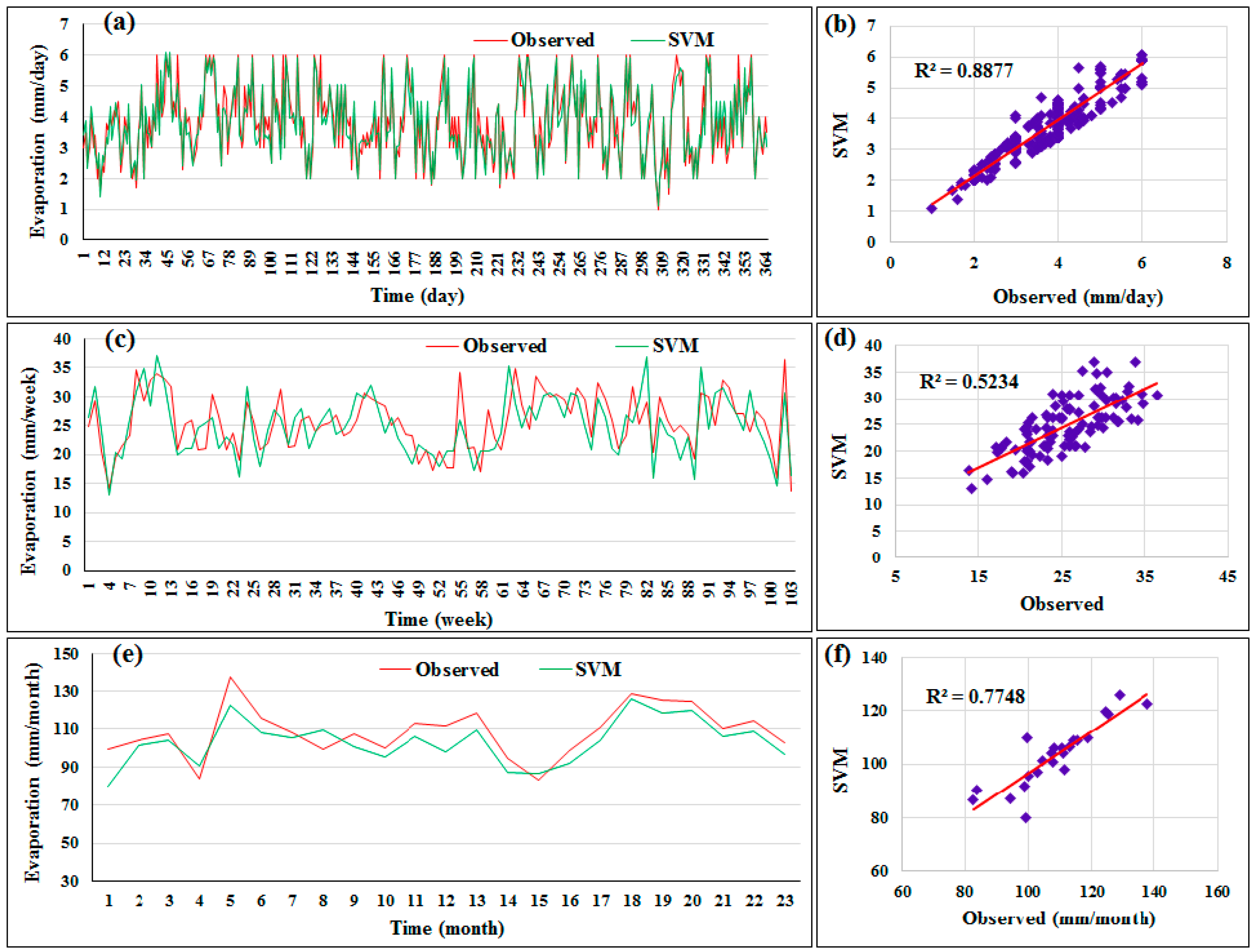
It is useful to present the distribution of the evaporation data which was predicted by the proposed models around a fit line. The pattern of the predicted data obtained by SVR versus actual evaporation is presented in Figure 4: (a) daily, (c) weekly, and (e) monthly. It can be seen that the suggested predictive model (i.e., SVR) was better with daily data at detecting the actual data than the other timescales. The scatterplots for the best models under the three timescales employing SVR are also shown in Figure 4. It is noticeable that the correlation between predicted and actual data with daily records was higher than the weekly and monthly timescales.
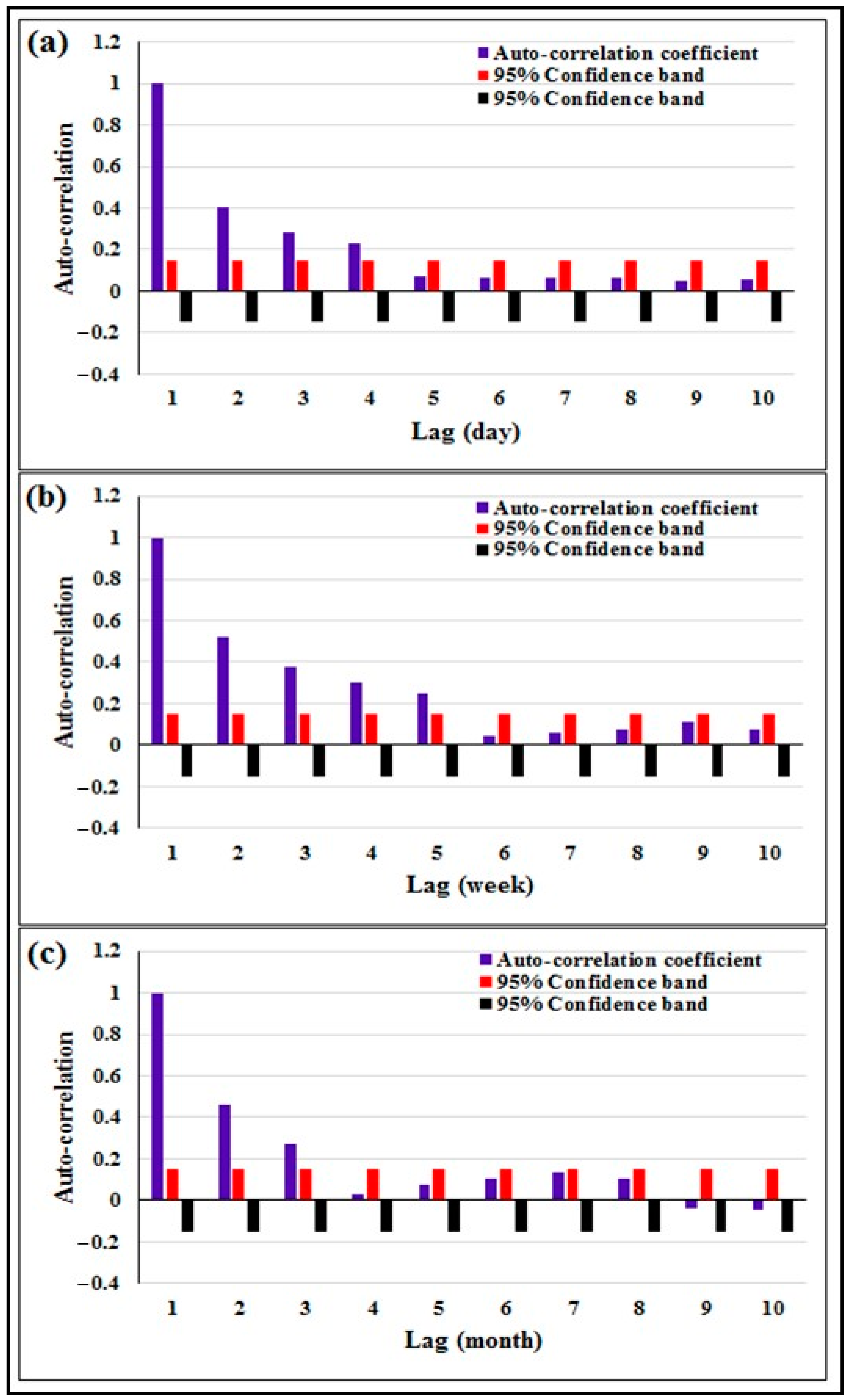
As the input variable(s) plays a significant role in the success of the model performance, it is essential as a first step to employ certain procedure to identify the proper input selection for the model for each time increment for the desired output. In this context, the model input selection variables were selected according to the autocorrelation procedure method. Mainly, the model is structured to consider three different time increments: daily, weekly and monthly. The autocorrelation procedure has been employed for all the time increment dataset. As a result, from the autocorrelation, for the case of daily time increment dataset, the output showed that there are four lags time has relatively strong correlation with the output. In this context, four different model input scenarios have been examined. While, for the weekly time increment, five lags time have correlation with the desired weekly output. Therefore, five different input scenarios have been applied in case weekly records. Finally, for the monthly time increment, only three lags have shown a strong correlation with the desired monthly output, and hence, only three different model scenarios have been applied for the monthly time increment. Consequently, the numbers of the examined models for each time increment are 4, 5 and 3 for daily, weekly and monthly time increment, respectively.
The RE% is a range falls between ± of the maximum experienced RE% for each model. The positive value of the RE% represents that the model is over-estimating the desired actual value of the output, while the negative value represents that the model is under-estimating the output.
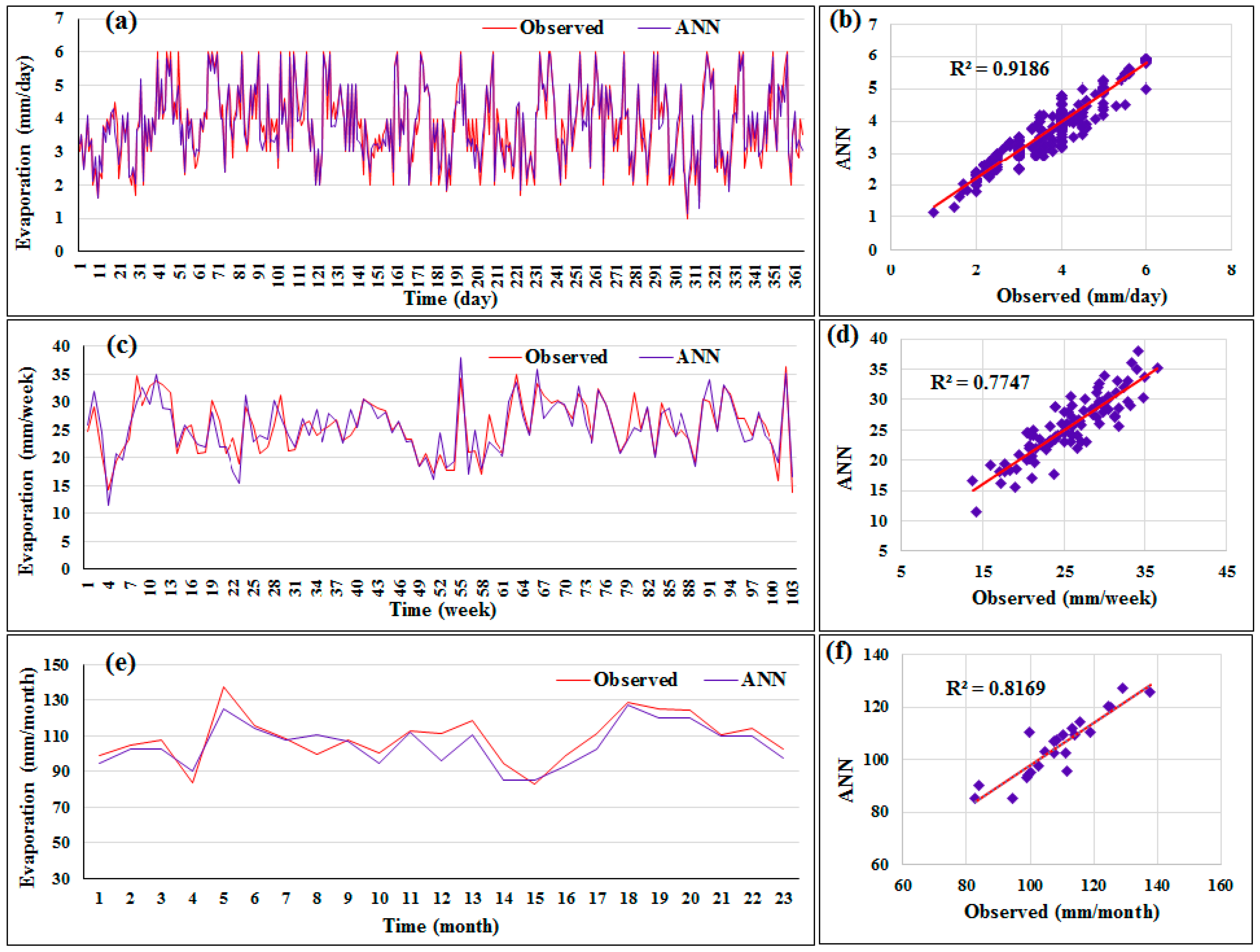
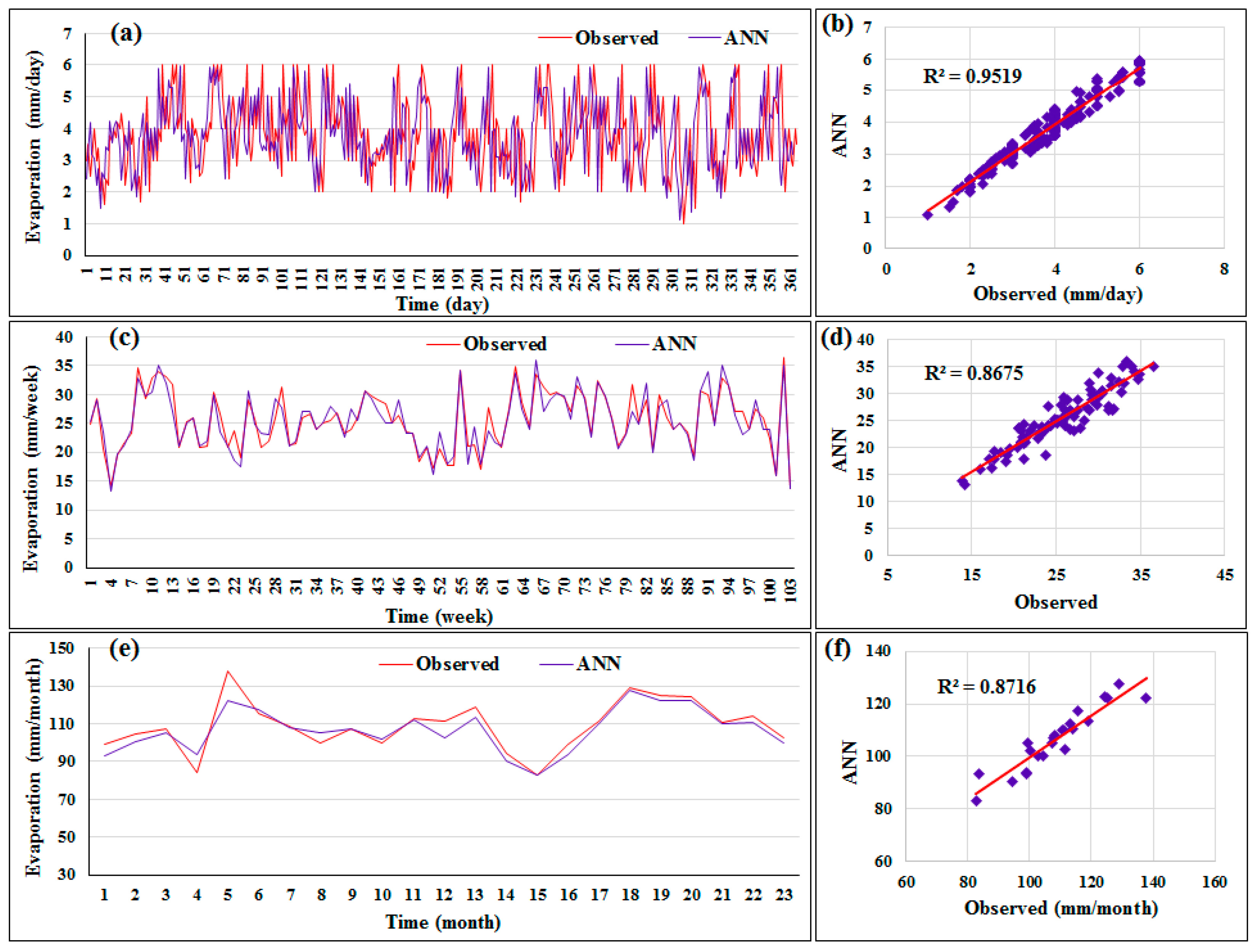
Figure 5 illustrates the hydrographs of the evaporation data predicted by the RBF-NN method with the best input combination within several time records (i.e., daily, weekly, and monthly). Most of the time, the predictions of the predictive model were underestimated when using monthly records. The best model (i.e., daily timescale) could predict the maximum values with acceptable accuracy, while the predictive model could not provide data to match with the medium data over the testing period as desired (Figure 5a). On the other hand, the scatterplots for the optimal model are shown in Figure 5. The proposed method (RBF-NN) provided the worst correlation between actual and predicted data when using weekly records (R2 = 0.774). Clearly, the agreement between the predicted and actual evaporation rate was significant with the daily timescale. Model III in daily scale has the best accuracy for both methods (RBF-NN and SVR) in all performance criteria. Where the best values of R2 NSE and KGE for SVR are (0.810, 0.781, and 0.795) respectively and for RBF-NN are (0.918, 0.942 and 0.932) respectively. It can be seen that the performance of the predictive model using daily records was superior to weekly and monthly records. Additionally, the accuracy of the results within the monthly timescale was better than weekly. This indicates that increasing the timescale may or may not improve the accuracy of the predictive model. Hence, inspecting the performance of the suggested models under several timescales is crucial.

4.2. Results of RBF-NN and SVR Scenario No. 2

The mean temperature and evaporation values were the modeling input variables in this scenario. Three multiscale time-series data (i.e., daily, weekly, and monthly) were used to train and test the models. Several models were suggested to determine the suitable input combination. The evaluation of all of the proposed models was carried out by examining their performance when using different statistical metrics.
Table 5 shows the results of the five models for each predictive model (i.e., SVR and RBF-NN). Firstly, the RMSE and MAE indicators demonstrated the reliability of the second model when using daily records and the third model when using weekly and monthly evaporation data. It can be seen that the correlation between the predicted and actual data using those models (Models II and III) was high compared with the other models. To check for any significant effects of the input variables on the performance of the methods and to compare the suggested models, the relative error magnitude was calculated for each model. The relative error indicated the superiority of the methods that used two and three input variables (i.e., Models II and III).
The proposed model that employed two input parameters using daily data had the smallest RMSE and MAE and the highest R2. This shows that the input combinations (E(t−1), E(t−2), T(t−1), T(t−2)) enhanced the performance of the predictive model. As seen in Table 5, using weekly and monthly data provided poor predictions. Therefore, it is pertinent to consider the influence of the timescale on the accuracy of results. On the other hand, the RBF-NN outperformed the SVR technique, according to the four indices (RMSE = 0.281 mm/day; MAE = 0.0201 mm/day; RE% = +11, −12; and R2 = 0.95). Model II in daily scale has the best accuracy for both methods (RBF-NN and SVR) where the best values of R2 NSE and KGE for SVR are (0.887, 0.912, and 0.892) respectively and for RBF-NN are (0.951, 0.968 and 0.935) respectively.
The patterns of the predicted data obtained by the architecture of the SVM models which led to the best results using different timescales are shown in Figure 6. These patterns demonstrate the flexibility and capability of SVR for mapping and predicting linear or nonlinear functions when using daily data. The scatterplots of the best model under the three timescales are also presented in Figure 6. It is observed that the SVM provided poor matching between the predicted and actual evaporation data using weekly records. The suggested method (i.e., SVM) was highly capable of predicting the evaporation values, which were less than 4 mm/day (Figure 6b). Finally, a high correlation magnitude was attained by employing daily evaporation data for modeling.
Figure 7 shows the distribution of the evaporation data predicted by the best model among all timescales (daily, weekly, and monthly). As seen in Figure 7a, the predicted and actual evaporation data converged, with the exception of some peak values. The performance of the proposed method with monthly data was slightly better than with weekly records. It was found that the correlation coefficient by the ANN method was 0.95. This magnitude of correlation was an adequate achievement in terms of the usability of the suggested model in predicting evaporation data in situations where indirect or direct methods cannot be used. The figures show that there was fairly good agreement between the predicted and actual data when using daily timescale data. Additionally, the improvement in the performance of the suggested method was attained with daily evaporation data. This demonstrates the ability of the ANN method to detect patterns in time-series data when using a lower timescale.

4.3. Comparison of the Models

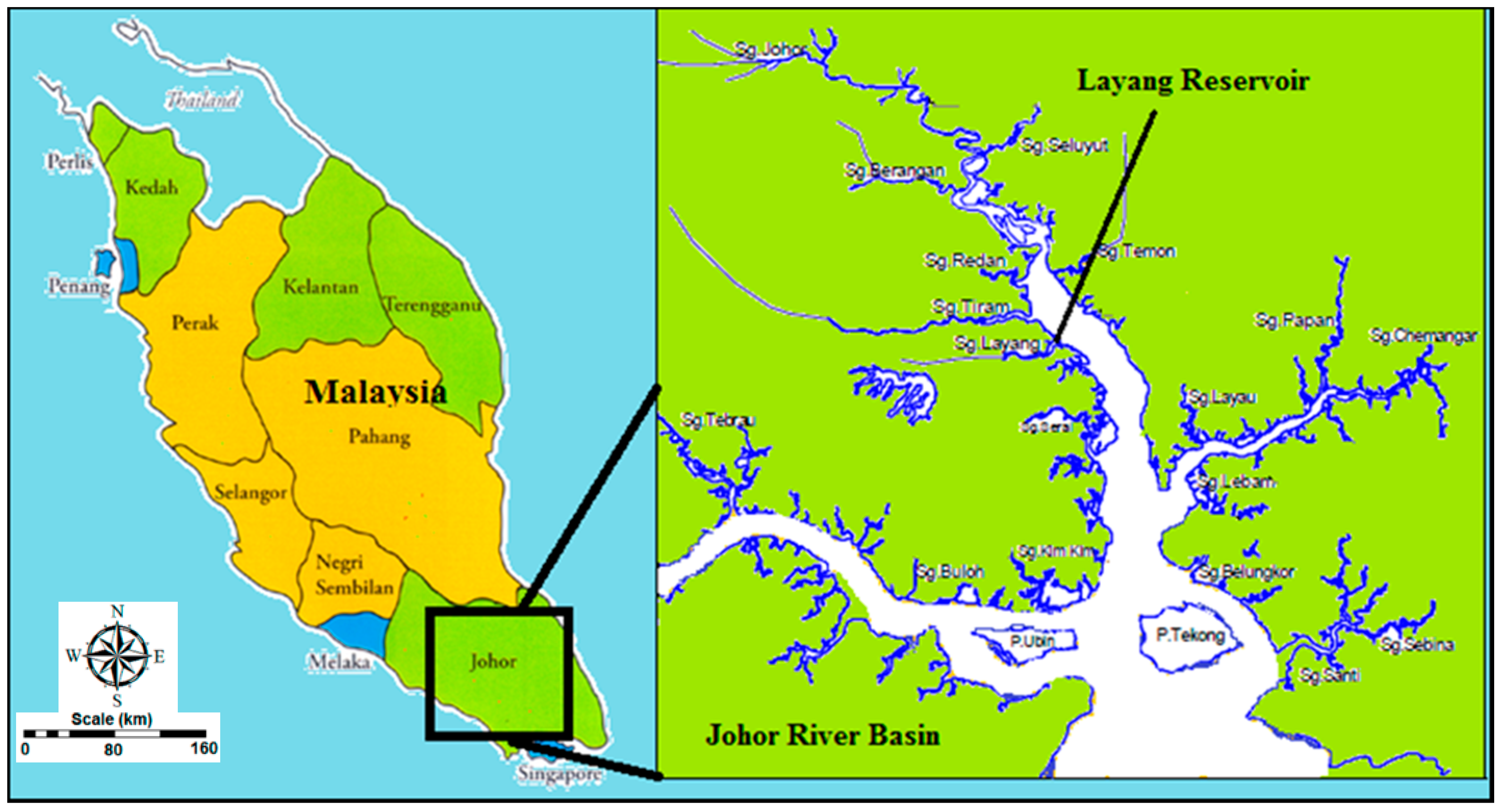
Ten-year evaporation and temperature data was used to predict the magnitude of evaporation from the reservoir in the future. A one-step prediction was attained for a one-year prediction period. To evaluate the performance of the suggested AI methods, two sceneries and three timescales were considered when predicting evaporation data. Noise reduction was not performed in the current study to investigate the performance of the method under hard conditions or with complex data. Therefore, the SVR and ANN techniques may provide greater accuracy than the current results when applied to noise-free evaporation data.
Four comparisons were carried out in this study: (i) comparing the optimal input combinations for the predictive model; (ii) comparing timescale suitability for modeling (iii) comparing two different input architectures (i.e., Scenario Nos. 1 and 2); and (iv) comparing the performances of the SVR and RBF-NN methods.
Firstly, the results in the first scenario revealed that three, four, and two input variables were the optimal input combinations for daily, weekly, and monthly timescales, respectively. In the second scenario, Model II for the daily basis and Model II for the weekly and monthly data were the best input variables for the predictive model.
In the light of the abovementioned results, the effect that the time increments had on the performance of the methods for evaporation prediction is clear. Table 4 and Table 5 show that using daily records increased the reliability of the AI techniques more so than weekly and monthly evaporation data. The optimal input combination models attained a high correlation between the predicted and actual data when employing the daily timescale. In addition, the minimum prediction error was obtained with daily records with both methods.
It is known that the meteorological data have a considerable effect on evaporation magnitude estimations. Indeed, the records of one or more climate parameters might not be available in many study areas due to a lack of monitoring devices to measure such parameters. Therefore, the current study attempted to provide a predictive model that can still be highly accurate even with minimal climate parameters. The accuracy of the results was significantly improved in the second section compared with the first section of the research by both SVR and RBF-NN models over the test period. Clearly, prediction errors were reduced when considering the temperature values in the evaporation prediction.
Based on the aforementioned results, it should be pointed out that the RBF-NN presented in the current study is very useful for solving the evaporation prediction problem. It is quite clear that the RBF-NN method attained all the planned objectives along with some interesting findings. It can be seen that the more complicated SVR method did not perform better. The capability of the RBF-NN in predicting evaporation data was superior to the SVR method. Furthermore, the main advantage of using the RBF-NN method is that it does not need detailed information on the physical processes of the system, unlike other methods, while the SVR method can achieve high accuracy only when feeding the model most of the effecting variables.
The relative error is an important indicator for evaluating the performance of the suggested methods. Therefore, the evaluation ranking of all proposed models was carried out based on the magnitude of the relative error. Table 6 illustrates the ranking of the models based on predicting monthly, weekly, and daily evaporation. The results showed that the RBF-NN (i.e., Model II, daily basis, under second scenario), with a relative error of 12%, was the best model for evaporation prediction in the current study. The second-best model was attained by feeding the RBF-NN with three input variables (i.e., E(t−1), E(t−2), and E(t−3)). The RBF-NN with daily records employing E(t−1) and T(t−1) as input variables was the third-best model, followed by the same model but under Scenario No. 1 with an REmax value of 19.5%. In fifth place was the SVR method considering two input variables, daily data, and under the second scenario. The SVR and RBF-NN methods were in sixth and seventh place when applying the SVR with Model III and RBF-NN with Model II under the first scenario with daily data, for which the magnitude of the relative error was 20.2% and 20.8%, respectively. It could be observable that the daily records are more suitable for the prediction models to attain accurate results. It seems that the prediction of the evaporation using small time scale (i.e., daily) is more understandable for the RBF-NN and SVR. The RBF-NN model was efficient even with minimum input variable. This indicates that the RBF-NN model could be better in case add some modifications for its procedure.
It can be seen from Table 6 that the 33rd to 46th places were mostly under Scenario No. 1. Finally, the RBF-NN method which considered the effect of temperature data and daily records succeeded in predicting the amount of water loss in a reservoir by way of evaporation within a tropical environment.

5. Conclusions

Predication of evaporation data is a vital requirement for water resources planning and management and everyday decision-tasks implemented in real hydrological practices. The accuracy of models used for evaporation predication is critical because an accurate for this parameter predict with early time can provide advanced warning of an impending drought at an early enough stage such that damage can be reduced significantly.
The objective of the current study was to examine the SVM and ANN models’ capacity for evaporation prediction. This research attempted to develop a powerful model that could predict evaporation data when missing one or more hydrological/ meteorological parameters. Two scenarios were considered to explore the performance of the suggested models. The results showed that taking into account the effect of temperature data as input variables for modeling enhanced the prediction accuracy. Clearly, the type of timescale had a significant effect on the performance of the models. Among the three timescales used, daily evaporation data improved the reliability of the predictive model when predicting evaporation. The comparison revelated that there was better agreement between the results of the RBF-NN model with actual evaporation data than those of the SVR method. The utilization of several distinct data input combinations and the subsequent modeling procedures enabled a robust extraction of the data attributes necessary to attain the most accurate predictive model. The present results showed that the predicted data attained by the RBF-NN model that used the input structure for Model II (with E P = E a ( t 1 ) , E a ( t 2 ) ,   T a ( t 1 ) ,   T a ( t 2 ) with daily records) were the most accurate when compared with other input combinations.
It should be pointed out that although the methodology presented here was mostly used to repair and extend the measured evaporation data, this scheme could be used to determine substantial contributing variables when developing empirical equations that can be used to estimate water losses from reservoirs. It could be concluded that the RBF-NN model is superior the SVR in predicting evaporation data. However, the proposed prediction model (i.e., RBF-NN) needs more modifications to be able to provide high-level accuracy. Further improvements could be introduced to improve the prediction accuracy such as training approach, input selection method and pre-pressing approach. Selection the suitable training period to learn the prediction model plays role to attain good results. Utilization the proper input selection approach also improved the prediction results. The ability of the prediction model could be improved by reducing the noise of the original data by using pre-processing approach. These approaches are likely to lead to a more robust prediction model that is responsive to the attributes within the input data, hence yield more accurate performance.

Author Contributions

Formal analysis, F.B.O., H.A.A., A.N.A. and M.S.H.; Methodology, M.F.A. and A.E.-S.; Writing—original draft, M.F.A. and C.M.F.; Writing—review & editing, H.A.A.

Funding

The authors would like to appreciate the financial support received from Bold 2025 grant coded RJO 10436494 by Innovation & Research Management Center (iRMC), Universiti Tenaga Nasional, Malaysia and from research grant coded UMRG RP025A-18SUS funded by the University of Malaya.

Acknowledgments

The authors appreciate so much the facilities support by the Civil Engineering Department, Faculty of Engineering, University of Malaya, Malaysia.

Conflicts of Interest

The authors declare no conflicts of interest.

Abbreviations

AHDAswan High Dam
AIArtificial Intelligence
ANFISAdaptive Neuro-Fuzzy Inference System
ANNArtificial Neural Networks
DIDDepartment of Irrigation and Drainage
ELMExtreme Learning Machine
FFNNFeedforward Neural Networks
GRNNGeneralized Regression Neural Networks
LS-SVMLeast Square Support Vector Machines
MAEMean Absolute Error
MLP-NNMultilayer Perceptron Neural Network
MSEMean Square Error
PEPan Evaporation
RBF-NNRadial Basis Function Neural Network
RBRadial Basis
RERelative Error
RMSERoot Mean Square Error
SVRSupport Vector Regression

References

  1. Friedrich, K.; Grossman, R.L.; Huntington, J.; Blanken, P.D.; Lenters, J.; Holman, K.D.; Gochis, D.; Livneh, B.; Prairie, J.; Skeie, E.; et al. Reservoir Evaporation in the Western United States: Current Science, Challenges, and Future Needs. Bull. Am. Meteorol. Soc. 2018, 99, 167–187. [Google Scholar] [CrossRef]
  2. Kohli, A.; Frenken AQUASTAT Programme, K. Evaporation from Artificial Lakes and Reservoirs; Food and Agriculture Organization: Rome, Italy, 2015. [Google Scholar]
  3. Zarei, G.; Homaee, M.; Liaghat, A.M.; Hoorfar, A.H. A model for soil surface evaporation based on Campbell’s retention curve. J. Hydrol. 2010, 380, 356–361. [Google Scholar] [CrossRef]
  4. Quinn, R.; Parker, A.; Rushton, K. Evaporation from bare soil: Lysimeter experiments in sand dams interpreted using conceptual and numerical models. J. Hydrol. 2018, 564, 909–915. [Google Scholar] [CrossRef]
  5. Rianna, G.; Reder, A.; Pagano, L. Estimating actual and potential bare soil evaporation from silty pyroclastic soils: Towards improved landslide prediction. J. Hydrol. 2018, 562, 193–209. [Google Scholar] [CrossRef]
  6. Allawi, M.F.; El-Shafie, A. Utilizing RBF-NN and ANFIS Methods for Multi-Lead ahead Prediction Model of Evaporation from Reservoir. Water Resour. Manag. 2016, 1–16. [Google Scholar] [CrossRef]
  7. Elzwayie, A.; El-shafie, A.; Yaseen, Z.M.; Afan, H.A.; Allawi, M.F. RBFNN-based model for heavy metal prediction for different climatic and pollution conditions. Neural Comput. Appl. 2016, 1–13. [Google Scholar] [CrossRef]
  8. Yaseen, Z.M.; Jaafar, O.; Deo, R.C.; Kisi, O.; Adamowski, J.; Quilty, J.; El-Shafie, A. Stream-flow forecasting using extreme learning machines: A case study in a semi-arid region in Iraq. J. Hydrol. 2016, 542, 603–614. [Google Scholar] [CrossRef]
  9. Yaseen, Z.M.; Allawi, M.F.; Yousif, A.A.; Jaafar, O.; Hamzah, F.M.; El-Shafie, A. Non-tuned machine learning approach for hydrological time series forecasting. Neural Comput. Appl. 2016, 1–13. [Google Scholar] [CrossRef]
  10. Afan, H.A.; El-Shafie, A.; Yaseen, Z.M.; Hameed, M.M.; Wan Mohtar, W.H.M.; Hussain, A.; Mohtar, W.H.; Hussain, A. ANN Based Sediment Prediction Model Utilizing Different Input Scenarios. Water Resour. Manag. 2014, 29, 1231–1245. [Google Scholar] [CrossRef]
  11. Ehteram, M.; Allawi, M.F.; Karami, H.; Mousavi, S.-F.; Emami, M.; EL-Shafie, A.; Farzin, S. Optimization of Chain-Reservoirs’ Operation with a New Approach in Artificial Intelligence. Water Resour. Manag. 2017, 31, 2085–2104. [Google Scholar] [CrossRef]
  12. Keskin, M.E.; Terzi, Ö.; Taylan, D. Fuzzy logic model approaches to daily pan evaporation estimation in western Turkey / Estimation de l’évaporation journalière du bac dans l’Ouest de la Turquie par des modèles à base de logique floue. Hydrol. Sci. J. 2004, 49. [Google Scholar] [CrossRef]
  13. Kim, S.; Kim, H. Neural networks and genetic algorithm approach for nonlinear evaporation and evapotranspiration modeling. J. Hydrol. 2008, 351, 299–317. [Google Scholar] [CrossRef]
  14. Kişi, Ö. Modeling monthly evaporation using two different neural computing techniques. Irrig. Sci. 2009, 27, 417–430. [Google Scholar] [CrossRef]
  15. Guven, A.; Kişi, Ö. Daily pan evaporation modeling using linear genetic programming technique. Irrig. Sci. 2011, 29, 135–145. [Google Scholar] [CrossRef]
  16. Samui, P. Application of least square support vector machine (LSSVM) for determination of evaporation losses in reservoirs. Engineering 2011, 3, 431–434. [Google Scholar] [CrossRef]
  17. Moghaddamnia, A.; Gousheh, M.; Piri, J.; Amin, S. Evaporation estimation using artificial neural networks and adaptive neuro-fuzzy inference system techniques. Adv. Water 2009, 32, 88–97. [Google Scholar] [CrossRef]
  18. Eslamian, S.; Abedi-Koupai, J. Estimation of Daily Reference Evapotranspiration Using Support Vector Machines and Artificial Neural Networks in Greenhouse. Res. J. 2009, 3, 439–447. [Google Scholar] [Green Version]
  19. Allawi, M.F.; Jaafar, O.; Mohamad Hamzah, F.; El-Shafie, A. Novel reservoir system simulation procedure for gap minimization between water supply and demand. J. Clean. Prod. 2019, 206, 928–943. [Google Scholar] [CrossRef]
  20. Allawi, M.F.; Jaafar, O.; Mohamad Hamzah, F.; Koting, S.B.; Mohd, N.S.B.; El-Shafie, A. Forecasting hydrological parameters for reservoir system utilizing artificial intelligent models and exploring their influence on operation performance. Knowl.-Based Syst. 2019, 163, 907–926. [Google Scholar] [CrossRef]
  21. Aljanabi, Q.A.; Chik, Z.; Allawi, M.F.; El-Shafie, A.H.; Ahmed, A.N.; El-Shafie, A. Support vector regression-based model for prediction of behavior stone column parameters in soft clay under highway embankment. Neural Comput. Appl. 2017, 1–11. [Google Scholar] [CrossRef]
  22. Keshtegar, B.; Allawi, M.F.; Afan, H.A.; El-Shafie, A. Optimized River Stream-Flow Forecasting Model Utilizing High-Order Response Surface Method. Water Resour. Manag. 2016, 30, 3899–3914. [Google Scholar] [CrossRef]
  23. Gupta, H.V.; Kling, H.; Yilmaz, K.K.; Martinez, G.F. Decomposition of the mean squared error and NSE performance criteria: Implications for improving hydrological modelling. J. Hydrol. 2009, 377, 80–91. [Google Scholar] [CrossRef] [Green Version]
Figure 1. Layang Reservoir at Johor River Basin is located at the southeast of Peninsular Malaysia.
Water 11 01226 g001
Figure 2. The architecture of Radial basis function neural network.
Water 11 01226 g002
Figure 3. Autocorrelation functions of the evaporation series (a) for daily data (b) for weekly data (c) for monthly data.
Water 11 01226 g003
Figure 4. The distribution of the predicted evaporation data by SVM method for the first scenario. (a) predicted pattern versus actual data within daily (c) weekly records, (e) monthly; (b) scatterplot for the evaporation data within daily time scale, (d) weekly, (f) monthly data.
Water 11 01226 g004
Figure 5. The distribution of the predicted evaporation data by (RBF-NN) method for the first scenario. (a) predicted pattern versus actual data within daily (c) weekly records, (e) monthly; (b) scatterplot for the evaporation data within daily time scale, (d) weekly, (f) monthly data.
Water 11 01226 g005
Figure 6. The distribution of the predicted evaporation data by SVM method for the second scenario. (a) predicted pattern versus actual data within daily (c) weekly records, (e) monthly; (b) scatterplot for the evaporation data within daily time scale, (d) weekly, (f) monthly data.
Water 11 01226 g006
Figure 7. The distribution of the predicted evaporation data by ANN (RBF-NN) method for the second scenario. (a) predicted pattern versus actual data within daily (c) weekly records, (e) monthly; (b) scatterplot for the evaporation data within daily time scale, (d) weekly, (c) monthly data).
Water 11 01226 g007
Table 1. Analysis of the evaporation data for the study area.
Time ScaleXmeanSxCv (Sx/Xmean)CsxXmaxXminMedian
Daily3.3611.2150.3610.43180.83
Weekly23.5275.020.2130.39641.911.422.85
Monthly100.63713.3860.1330.119137.766.799.85
Note: Xmean = mean value; Sx = standard deviation; Cv = coefficient of variation; Csx = skewness; Xmin = minimum value and Xmax = maximum value.
Table 2. The input combination for each suggested model in the first scenario.
ModelInput CombinationOutput
Model IE(t−1)E(t)
Model IIE(t−1), E(t−2)E(t)
Model IIIE(t−1), E(t−2), E(t−3)E(t)
Model IVE(t−1), E(t−2), E(t−3), E(t−4)E(t)
Model VE(t−1), E(t−2), E(t−3), E(t−4), E(t−5)E(t)
Table 3. The input combination for each suggested model in the second scenario.
ModelInput CombinationOutput
Model IE(t−1), T(t−1)E(t)
Model IIE(t−1), E(t−2), T(t−1), T(t−2)E(t)
Model IIIE(t−1), E(t−2), E(t−3), T(t−1), T(t−2), T(t−3)E(t)
Model IVE(t−1), E(t−2), E(t−3), E(t−4), T(t−1), T(t−2), T(t−3), T(t−4)E(t)
Model VE(t−1), E(t−2), E(t−3), E(t−4), E(t−5), T(t−1), T(t−2), T(t−3), T(t−4), T(t−5)E(t)
Table 4. The performance criteria (RMSE, MAE, R2 and RE %) values for Scenario No. 1 using RBF-NN and SVR methods.
Time IncrementInput ModelsSVRRBF-NN
RMSEMAER2RE %NSEKGERMSEMAER2RE %NSEKGE
DailyModel I0.6900.0990.802+21.2, −260.7420.7650.4320.0220.875+19.6, −18.30.8520.812
Model II0.8080.0600.802+22.8, −21.40.7530.7710.8200.0420.872+20.8, −20.30.8830.857
Model III0.5160.0420.810+20.2, −19.80.7810.7950.3180.0210.918+18, −18.50.9420.932
Model IV2.2100.1150.675+23.7, −26.40.6420.6542.1100.1100.781+22, −25.40.8030.798
WeeklyModel I1.0430.1020.342+39.5, −39.20.4280.4531.8450.1800.775+38.4, −36.20.7810.732
Model II2.0570.2020.338+37.4, −36.20.3650.3142.4090.2360.768+36.8, −35.30.7580.748
Model III1.5610.1530.340+37, −36.80.3370.3273.1010.3050.730+36.6, −34.80.7420.763
Model IV0.8870.0860.347+35.3, −33.60.3820.3580.7340.0720.774+34, −32.50.8020.772
Model V0.9440.0930.386+37.8, −38.70.4120.4024.2170.4150.794+36.4, −38.20.7870.754
MonthlyModel I8.9311.8230.410+36.4, −35.30.4830.4374.8870.9970.664+33.4, −31.30.6310.657
Model II3.6750.7500.503+30.5, −29.70.5210.5371.3400.2790.81628.7, −27.30.8240.784
Model III10.7192.2350.468+33, −34.50.4830.4381.4970.3050.783+32.3, −31.20.7950.762
(MAE) Mean Absolute Error; (MSE) Mean Square Error; (RE) Relative Error; (RMSE)Root Mean Square Error; (R2)correlation coefficient; (NSE) Nash-Sutcliffe efficiency and (KGE’) modified Kling-Gupta efficiency.
Table 5. The performance criteria (RMSE, MAE, R2 and RE %) values for Scenario No. 2 using RBF-NN and SVR methods.
Time IncrementInput ModelsSVRRBF-NN
RMSEMAER2RE %NSEKGERMSEMAER2RE %NSEKGE
DailyModel I0.9550.0870.897+20, −250.8720.8630.5420.0440.904+19.5, −18.30.9130.884
Model II0.4210.0320.887+18, −200.9120.8910.2810.0200.951+11, −120.9680.935
Model III1.0110.0880.884+23.4, −27.80.9010.8540.9250.0920.879+20.3, −22.70.8420.852
Model IV1.2351.0740.812+46, −450.7830.8271.0780.9470.851+41, −42.40.7930.835
Model V1.8641.9420.721+57, −46.50.7570.7431.1431.0480.774+40.5, −430.7360.783
WeeklyModel I1.2040.1210.501+26.8, −29.40.4820.5270.7540.0680.878+25.7, −26.20.8210.858
Model II1.0020.0850.513+25.4, −280.5370.5480.6620.0610.880+24.8, −25.30.9020.885
Model III0.6560.0420.523+25, −26.30.5410.5720.5240.0450.867+24.6, −23.80.9270.908
Model IV0.6950.0480.516+29.4, −31.20.5370.4930.7110.0670.872+28.7, −29.80.8280.853
Model V1.9242.0730.483+61, −68.60.4920.5241.1771.0690.845+43.8, −42.50.7810.812
MonthlyModel I5.2310.9520.643+26.6, −240.6740.6284.3280.9850.452+26.5, −23.50.4020.483
Model II2.8210.8570.657+27.9, −22.30.6480.6732.3250.7210.523+24.2, −23.20.4980.557
Model III1.3540.4240.778+22, −220.7930.8041.1120.2410.871+21.3, −19.80.9070.892
Model IV2.8230.9250.703+23, −240.6850.7121.3340.2950.584+25.6, −24.50.5180.547
Model V3.2581.8920.521+51, −63.20.5470.5722.8711.3280.542+43.5, −58.30.4870.538
Table 6. Summary ranking for all models with three time scales.
RankMethodNo. of ModelScale TimeNo. of Scenario
1RBF-NNModel IIDaily2
2RBF-NNModel IIIDaily1
3RBF-NNModel IDaily2
4RBF-NNModel IDaily1
5SVRModel IIDaily2
6SVRModel IIIDaily1
7RBF-NNModel IIDaily1
8RBF-NNModel IIIMonthly2
9SVRModel IIIMonthly2
10RBF-NNModel IIIDaily2
11SVRModel IIDaily1
12SVRModel IVMonthly2
13RBF-NNModel IIMonthly2
14RBF-NNModel IIIWeekly2
15RBF-NNModel IIWeekly2
16SVRModel IDaily2
17RBF-NNModel IVDaily1
18RBF-NNModel IVMonthly2
19SVRModel IDaily1
20RBF-NNModel IWeekly2
21SVRModel IIIWeekly2
22SVRModel IVWeekly1
23RBF-NNModel IMonthly2
24SVRModel IMonthly2
25SVRModel IIIDaily2
26SVRModel IIMonthly2
27SVRModel IIWeekly2
28RBF-NNModel IIMonthly1
29SVRModel IWeekly2
30RBF-NNModel IVWeekly2
31SVRModel IIMonthly1
32SVRModel IVWeekly2
33RBF-NNModel IIIMonthly1
34RBF-NNModel IMonthly1
35RBF-NNModel IVWeekly1
36SVRModel IIIMonthly1
37SVRModel IVWeekly1
38SVRModel IMonthly1
39RBF-NNModel IIIWeekly1
40RBF-NNModel IIWeekly1
41SVRModel IIIWeekly1
42SVRModel IIWeekly1
43RBF-NNModel VWeekly1
44RBF-NNModel IWeekly1
45SVRModel VWeekly1
46SVRModel IWeekly1
47RBF-NNModel IVDaily2
48RBF-NNModel VDaily2
49RBF-NNModel VWeekly2
50SVRModel IVDaily2
51SVRModel VDaily2
52SVRModel VWeekly2
53RBF-NNModel VMonthly2
54SVRModel VMonthly2

