Article

Water Quality Prediction Model Based Support Vector Machine Model for Ungauged River Catchment under Dual Scenarios

by
Abobakr Saeed Abobakr Yahya
1,
Ali Najah Ahmed
1,*,
Faridah Binti Othman
2,
Rusul Khaleel Ibrahim
2,
Haitham Abdulmohsin Afan
2,*,
Amr El-Shafie
3,
Chow Ming Fai
1,
Md Shabbir Hossain
4,
Mohammad Ehteram
5 and
Ahmed Elshafie
2
1
Institute of Energy Infrastructure (IEI), Universiti Tenaga Nasional, Kajang 43000, Selangor, Malaysia
2
Department of Civil Engineering, Faculty of Engineering, University Malaya, Kuala Lumpur 50603, Malaysia
3
Civil Engineering Department El-Gazeera High Institute for Engineering Al Moqattam, Cairo 11311, Egypt
4
Department of Civil Engineering, School of Energy, Geoscience, Infrastructure and Society, Heriot-Watt University, Putrajaya 62200, Malaysia
5
Department of Water Engineering and Hydraulic Structures, Faculty of Civil Engineering, Semnan University, Semnan 35131-19111, Iran
*
Authors to whom correspondence should be addressed.
Water 2019, 11(6), 1231; https://doi.org/10.3390/w11061231
Submission received: 29 April 2019 / Revised: 14 May 2019 / Accepted: 15 May 2019 / Published: 13 June 2019

Abstract

:
Water quality analysis is a crucial step in water resources management and needs to be addressed urgently to control any pollution that may adversely affect the ecosystem and to ensure the environmental standards are being met. Thus, this work is an attempt to develop an efficient model using support vector machine (SVM) to predict the water quality of Langat River Basin through the analysis of the data of six parameters of dual reservoirs that are located in the catchment. The proposed model could be considered as an effective tool for identifying the water quality status for the river catchment area. In addition, the major advantage of the proposed model is that it could be useful for ungauged catchments or those lacking enough numbers of monitoring stations for water quality parameters. These parameters, namely pH, Suspended Solids (SS), Dissolved Oxygen (DO), Ammonia Nitrogen (AN), Chemical Oxygen Demand (COD), and Biochemical Oxygen Demand (BOD) were provided by the Malaysian Department of Environment (DOE). The differences between dual scenarios 1 and 2 depend on the information from prior stations to forecast DO levels for succeeding sites (Scenario 2). This scheme has the capacity to simulate water-quality accurately, with small prediction errors. The resulting correlation coefficient has maximum values of 0.998 and 0.979 after the application of Scenario 1. The approach with Type 1 SVM regression along with 10-fold cross-validation methods worked to generate precise results. The MSE value was found to be between 0.004 and 0.681, with Scenario 1 showing a better outcome.

1. Introduction

Water plays a crucial role in environmental and social life. It occupies the largest area of our planet, and therefore, among all other natural resources, water resources gain the most special place. However, the ongoing increase in urbanization and industrialization processes generate wide ranges of hazardous contaminants that deteriorate the quality of river waters. The produced wastes are discharged into water bodies in different forms, for instance, organic pollutants (pesticides, insecticides, phenols, hydrocarbons, etc.), heavy metals (lead, arsenic, copper, cadmium mercury, etc.), and microbial pathogens. All these water pollutants cause adverse effects on public health and the surrounding wildlife. Therefore, there is an exigent demand to monitor the levels of water quality. Rapid population growth and climate change in the past few decades resulted in the scarcity of fresh water, as well as degrading the water-quality levels across the globe [1]. The Water Quality Index (WQI) summarizes water quality information in a readily-understood scale format. Index numbers range between 1 and 100, wherein higher numbers indicate better water-quality levels. Generally, river stations that score 80 or more indicate that water quality meets expectations for “clean rivers”, stations that score from 40 to 80 indicate “slightly polluted rivers”, whereas river stations that score below 40 indicate that the water quality expectations are not being met, and are regarded as “polluted rivers”.
In past research, various water-quality parameters are integrated into a general index that forms the water-quality index (WQI). The development of WQI and its use in assessing water-quality levels have risen exponentially [2]. One of the challenges faced in recent researches on water quality is the need to reduce costs while developing smarter computer-aided means of assessing water-quality levels. WQI represents the best means to communicate and categorize water-quality levels in assessments of water suitability for various applications. Nevertheless, a variety of WQI types have been planned for quick and efficient assessments of the general level of water quality throughout particular regions. The WQI scale relied on by the Canadian Council of Ministers of Environment is utilized in Canada and many other countries [3].

1.1. Background

Polluted water has been widely spread all over the globe in the past few decades, and thus water-quality level assessment and forecasting have become more essential to the ecological management organisations of many countries. A set of six parameters is typically used in DOE analyses for evaluating surface water characteristics in terms of pH, Suspended Solids (SS), Dissolved Oxygen (DO), Ammonia Nitrogen (AN), Chemical Oxygen Demand (COD), and Biochemical Oxygen Demand (BOD). The prediction of water-quality parameters based on accurate values could enable better early cautionary of contaminated water and timely decision-making. To this day, dual scenarios are extensively employed to forecast water-quality trends. Scenario 1 is designed to validate the DO prediction scheme at each station according to five input parameters, while Scenario 2 is designed to validate the DO prediction scheme according to five input parameters as well as DO predictions from a prior (upstream) station [4,5,6].
In this study, time-series predictive techniques for water quality were discussed, which predict the value of water quality parameters at interval t through use of preceding time series, based on similar and other parameters. For many decades, numerous statistical analyses and AI-based modelling strategies have been used to influence time-series predictive techniques for water quality and in water resources management [6,7,8,9,10,11,12,13,14,15]. To this day, the term water quality is utilized for describing water conditions, such as physical, chemical, and biological properties. Among the most important factors for water quality is the dissolved oxygen (DO), which refers to the presence of oxygen gas molecules (O2) in terms of mg/L concentrations. Plant and animal species cannot directly utilise the oxygen that forms part of water molecules (H2O). The dissolved oxygen content can be decreased through respiration processes, wherein oxygen enters surface water from the air as a photosynthetic product of river plants. Generally, a constant high level of DO is best for ecosystems.
The level of DO varies according to many factors such as depth, altitude, and season, rates of flow, water temperatures, and time of the day. Water coursing at increased temperatures and at higher altitudes normally contains lesser amounts of DO. Moreover, DO levels peak during the daytime, whereas during night time, the DO levels lower along with the decreased photosynthetic action due to the oxygen-consuming activities including oxidation and respiration, until just before dawn. DO levels directly affect fish cultures: (1) At low DO levels (0–2 mg/L), oxygen is insufficient to support fish cultures; (2) at middle DO levels (2–4 mg/L), few river fish and insect species can survive; (3) at higher DO levels (4–7 mg/L), oxygen is sufficient to support diverse river life, particularly cold-water fish species; (4) For the majority of stream fish, the optimal DO range is 7–11 mg/L. Human activities that influence DO levels in surface water include the entry of additional oxygen-consuming organic wastes, including sewage, nutrient additions, changing water flows, rising water temperatures, and added chemicals [16].
Selangor, Malaysia, has long experience with river water pollution issues linked to land-use trends. The Langat River forms a principal basin that drains into densely-populated and highly-developed areas in Selangor. For four decades, the river has served almost half the populace of Selangor as a water supply and remains a source of hydroelectric power and flood discharge controls. More than two-thirds of the region’s population resides in the floodplain, which features highly fertile soil for agricultural as well as for industrial, residential, and recreational purposes. This situation has brought about conflict between economic development and river ecosystems, which has led to increasing amounts of wastes in riverine channels [17]. A total of 42 tributaries surveyed in Peninsular Malaysia are categorised as highly polluted, including Langat River Basin. In 1999, a total of 13 tributaries across Malaysia along with 36 rivers were polluted as a result of industrial, construction, and agricultural activities along the tributaries [18]. Until 1990, a total of 48 rivers could still be classified as clean, in comparison to only 32 that remained clean as of 1999 [15]. Some 60% of all main rivers are subject to regulation for residential, agricultural, and commercial purposes. The primary pollution sources in Malaysia that affect its river systems are sewage disposal, discharge from small- and medium-sized industries that improperly treat effluents, and various land-clearing and earthwork processes. By 1999, some 42% of all river basins were reportedly contaminated with suspended solids (SS) as a result of badly planned and controlled land-clearing processes, some 30% with heavy biological oxygen demand (BOD) due to industrial effluent, and some 28% with ammoniacal nitrogen (AN) due to animal husbandry activity and domestic disposal of sewage [19].
Surface water pollution has been identified as the primary problem that affects the Langat River. The expansion of human development in the basin has led to increased wastes entering its channels. In efforts to prevent further pollution, the Department of Environment (DOE), under Malaysia’s Ministry of Natural Resources and Environment, has set up telemetry stations all along the river in a programme that monitors the water-quality levels on a continuing basis. Based on water-quality data, the water-quality index (WQI) was applied in order to assess water-quality status and river category. The measure offers a useful basis for forecasting changes in water-quality levels, through the consideration of several factors. WQI comprises six water-quality level variables, including SS, pH, AN, dissolved oxygen (DO), chemical oxygen demand (COD), and biochemical oxygen demand (BOD) [14].

1.2. Problem Statement

The level of pollution has been increasing in Selangor with regards to the increased amounts of wastes entering the Langat River leading to water shortage within the basin. Numerous sources of wastes contaminate the Langat River, including emissions of industrial effluent that are 58% of all pollutants, with 28% discharged from domestic sewage treatment plants, while construction projects account for some 12% and pig farms only 2% of the total. In 2011, the WQI for Langat River was between 72 and 75, which led to its classification as a slightly polluted river. WQI remains at a class I level at the upstream station in the Hulu Langat District prior to the Lui River, which indicates a low-pollution area. However, WQI changes to a class III level at the downstream station past the Batang Benar and Balak tributaries [20]. This paper examines the efficiency of Support Vector Machine (SVM) models in predicting water-quality levels for Langat River within Malaysia. A network was devised and trained using six major parameters to estimate water-pollutant levels as well as water-quality levels and classes. Its dataset includes records that have been gathered over the past decade since 2006. Artificial Neural Network (ANN) and Support Vector Machine (SVM) systems have been used to forecast water-quality levels. SVM offers more advantages than its ANN equivalents, for it can resolve small samples in term of nonlinear, high-dimensional, localised minima, and other partial elements. SVM also features a modular scheme that enables independent implementation of component designs. This research demonstrates the use of SVM in forecasting water-quality characteristics based on these six parameters, with dynamic processes masked in the very measurement data.

1.3. Objectives

The objectives and goals of the project are as follows:
(1)
To provide effective methods of water-quality prediction to decision makers, towards better water resource planning and management.
(2)
To present a system-independent method of water-quality forecasting that utilises SVM in place of statistical modelling methods.
(3)
To provide recommendations to water-quality management agencies that accord with the research findings on the Langat River Basin, regarding how such findings may be integrated into ecological strategies for catchment management.

2. Materials and Methods

2.1. Case Study

The Langat basin (Figure 1) includes a key catchment that provides for raw water supplies and further resources to some 1.2 million people residing there. Key stretches serve various towns, namely Kajang, Cheras, Bangi, Putrajaya Government Centre, and so on. Dual reservoirs are located in the catchment, namely Semenyih and Hulu Langat Dam, along with eight water-treatment plants that provide for safe and clean and water supplies. Langat River features a total catchment area of some 2350 km² and is located at latitudes between 2°40′M 152″ N and 3°16′M 15″ N and along longitudes between 101°19′M 20″ E and 102°1′M 10″ E. The principal river has a length of 141 km that stretches some 40 km east of the capital of Kuala Lumpur and features several tributaries, the largest of which are the Lui, Semenyih, and Beranang Rivers. There are two reservoirs that the Langat and Semenyih dams supply via particular catchment. The newer Langat dam was constructed in 1981 with a catchment area totalling 54 km², whereas Semenyih was constructed in 1942 and features a catchment area totalling 41 km². The Langat River represents more than just a supply of water, for it serves further purposes that include recreational activities, fishing, irrigation, effluent discharge, as well as sand mining. As a result of the growth of numerous activities along its streams, it has become necessary to evaluate related water demand and resource supply.
This research investigates water-quality forecast methods for the Langat catchment, which drains into three major tributaries, the Langat, Semenyih, and Labu Rivers. Nevertheless, this research only covers the upper portion of the Langat catchment. The primary Langat tributary flows some 182 km from the major range (Banjaran Titiwangsa) in the northeast of Hulu, through Langat District in the south-southwest direction, and drains via the Straits of Malacca. The Langat and Semenyih Rivers both originate in hilly and forested regions along the western slopes of Banjaran Titiwangsa, which is northeast of the Hulu Langat District. Semenyih River runs mainly from the Semenyih Dam, in a stretch that flows south-southwest into and through the towns of Semenyih and Bangi Lama, which then joins with the Langat River some 4 km east of Bangi Lama. Semenyih River is joined by the Beranang and Pajam Rivers as well, and both originate in the northern area of the Seremban District, namely Negeri Sembilan. The data has been gathered from seven water stations along the Langat River.

2.2. Select Appropriate Inputs

The water-quality data utilized in this research was obtained through the Malaysian Department of Environment (DOE). Time-series data for selected parameter sets through four stations from 2006 until 2016 were utilized in this research. Six water-quality parameters were chosen for SVM modelling in this research, specifically pH, Suspended Solids (SS), Dissolved Oxygen (DO), Ammonia Nitrogen (AN), Chemical Oxygen Demand (COD), and Biochemical Oxygen Demand (BOD). Simple statistics for measured water-quality parameters in the Langat River from 2006 to 2016 are displayed in Table 1.

2.3. Structure of SVM

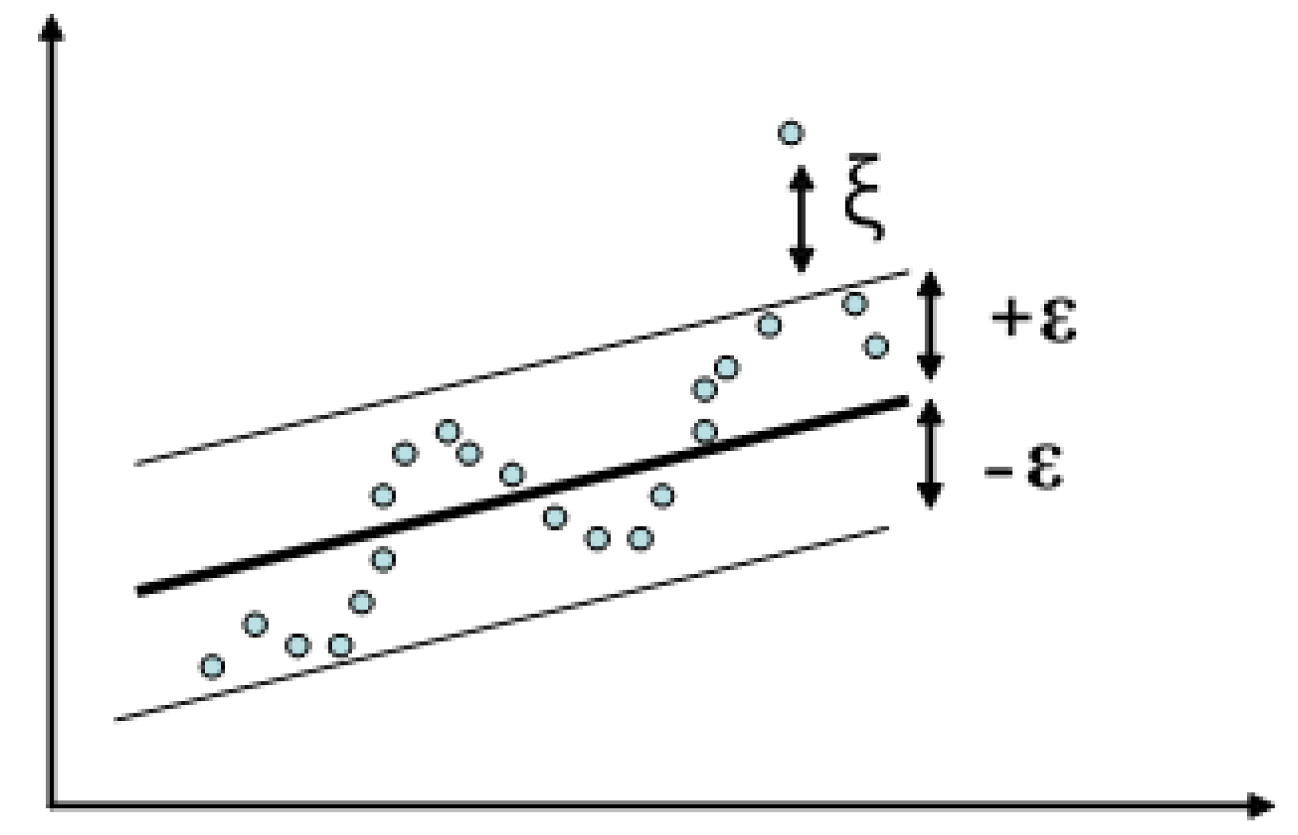
Support vectors are the training points that are the nearest to the separating hyperplane and the basic concept of SVM is illustrated in Figure 2. There are decision functions that are accountable for example, hyperplanes that are able to delineate the positive and negative data that has marked the maximum margins. This shows the range from the nearest positive sample to a hyperplane and the range between the nearest negative sample and the hyperplane shall be maximized [21].
y ( x ) = w T ϕ ( x ) + b
where, ϕ(x) represents the high dimensional feature spaces, which is nonlinearly mapped from the input space x. The coefficient are w and b are estimated by minimizing the regularized function R ( C ) :
R ( C ) = C 1 N i = 1 N L ε ( d i , y i ) + 1 2 w 2
where
L ε ( d i , y i ) = { | d i   y i | ε i f   | d i   y i | ε 0 o t h e r w i s e
To obtain the estimation of w and b, Equation (2) is transformed to the primal function given by Equation (4) by introducing the positive slack variables ξ i and ξ i as follows:
  M i n i m i z e :   R ( C ) = C ( i = 1 N ( ξ i + ξ i ) ) + 1 2 w 2
S u b j e c t   t o   { d i w ( x i ) b i   ε + ξ i ,   i = 1 , 2 , , N w ( x i ) + b i y i   ε + ξ i ,   i = 1 , 2 , , N ξ i , ξ i   0   i = 1 , 2 , , N
The first term (l/2‖w‖2) is the weights vector norm, d i the desired value, and C is referred as regularized constant determining the tradeoff between the empirical error and the regularized term. ε is called the tube size of SVM as shown in Figure 2.
It is similar to the equation accuracy that is related in the training data. The multipliers that are non zero are known as support vectors. This is where the variable slacks and brought into the study. ξ i and ξ i are introduced and by introducing this and by exploiting constraint optimality the function decision by Equation (1) gives the following:
y ( x ) = i = 1 N ( α i α i )   K   ( x , x i ) + b
In Equation (5), α i and α i , are the so-called Lagrange multipliers. They satisfy the equalities α i , × α i = 0, α i , ≥0 and α i ≥ 0 where, i = 1, 2, …, n and are obtained by maximizing the dual function of Equation (4) which has the following form:
R ( α i , α i ) = i = 1 N d i ( α i α i ) ε i = 1 N ( α i + α i ) 1 2 i = 1 N   j = 1 N d i ( α i α i )   ( α j α j )   K   ( x i , x j )
with the constraints
i = 1 N ( α i ) = i = 1 N ( α i )   a n d   α i , α i   [ 0 , C ] ,   i = 1 , 2 , , N
K   ( x i , x j ) is defined as the kernel function. The value of the kernel is equal to the inner product of two vectors x i and x j in the feature space ϕ(xi) and ϕ(xj), that is, K   ( x i , x j ) = ϕ(xi) × ϕ(xj).
Four common kernel function types of SVM are given as follows:
Linear   kernel :   K   ( x i , x j ) = x i T × x j
Polynomial   kernel :   K   ( x i , x j ) = ( γ x i T × x j + r ) d ,   γ > 0
Radial   basis   kernel :   K   ( x i , x j ) = exp ( x i x j   2 ) ,   γ > 0
Sigmoid   kernel :   k ( x i , x j ) = t a n h ( x i T × x j + r )
Here, γ , r and d are kernel parameters. The kernel parameters should be carefully chosen as it implicitly defines the structure of the high dimensional feature space ϕ(x) and thus controls the complexity of the final solution.
There are two types of SVM regression; both have the general formula given in Equation (1). The first type of SVM regression is known as Type 1 or Epsilon. This type of error function is given by the formula shown in Equation (4). The second type of regression is known as Nu.

2.4. Statistical Indexes

Model performances were assessed based on three statistical indexes.

2.4.1. Coefficient of Efficiency (CE)

To assess model performance, Coefficient of Efficiency (CE) was utilized [5].
C E = 1   i = 1 n ( m p ) 2 i = 1 n ( m m ¯ ) 2
wherein n is the number of observations, m and p correspond to the measured and predicted data, while m ¯ denotes the average of the measured data.

2.4.2. Mean Square Error (MSE)

Mean square error (MSE) is utilized to establish and define the fit of the network outputs to the desired scheme. Lower values for MSE enable higher performance (values nearer 0 indicate reliable and accurate results), which is expressed as follows:
M S E = 1 n i = 1 n ( m p ) 2

2.4.3. Coefficient of Correlation (CC)

Coefficient of correlation (CC) is utilized to assess the linear relationship between the observed and predicted data. It is defined as follows:
C C = i = 1 n ( m m ¯ ) ( p p ¯ ) i = 1 n ( m m ¯ ) 2 i = 1 n ( m p ¯ ) 2

2.5. Sensitivity Analysis

To assess the effect of input parameters on this model, dual evaluation processes are utilized. Firstly, performance evaluations for various possible parameter combinations are investigated using Mean Square Error (MSE) and Coefficient of Efficiency (CE) and methods, in order to establish the most effective parameters for the output. Generally, six networks were compared, each of which demonstrate the significance of eliminated parameters that influence network accuracy [22].

3. Results and Discussion

3.1. Kernel Functions of SVM

In this study, SVM was developed with the use of various kernel function types such as Linear, Polynomial, Radial Basis, and Sigmoid functions. Trial and error method were conducted in order to establish the best types of kernel functions through cross-validation-based processes. Table 2 displays a comparative analysis of predictive performances for the SVM model based on four different kernel function types. Regarding the coefficient of correlation value when utilising RBF kernel, the predictive precision of the test data was most reliable at around 0.801, followed by the Polynomial 0.496, Linear 0.438, and Sigmoid 0.336 kernels.

3.2. Epsilon-RBF Model and Nu-RBF Model

The search for model parameter sets does have a vital role in acquiring reliable predictive performances for SVM. Settings for hyper-parameters (C, γ) and kernel parameters (Nu and Epsilon) are considered to be vital in shaping SVM generalization performances (approximation accuracy).
In the search for the best SVM architecture for particular applications, dual test types exist for RBF kernel functions, namely Epsilon (ε) and Nu. Epsilon-RBF is utilized for predictions, so C is set to 8.5 and γ = 8, with ε set to values ranging from 0.001 to 0.5. Results for model performance in testing and training are displayed in Table 3, which shows that MSE increases with increases in values of ε while every correlation coefficient value and the numbers of support vectors decreases. Lastly, an ε value of 0.001 yields minimal generalization errors, with acceptable numbers of the support vector (36) selected. Where the Nu model increases, the predictive precision of the test data will gradually rise to its highest value (at Nu = 0.4), with the remaining values set as displayed. Table 4 also displays the numbers that associate with support vectors increasing as Nu values increase. In accordance with these results, it is noted that the best-fitting values for correlation coefficient and MSE correspond to 0.998 and 0.001, respectively, where obtained by utilizing Nu-RBF Model with Gamma equal to 8 and Capacity equal to 8.5.

3.3. Optimising the Parameters of SVM

There are two essential parameters that are required to be selected in order to achieve the best structure of the SVM model. These parameters are gamma γ and capacity parameter C. The prediction accuracy shows a very high sensitivity to the selection of C, as a small value of C can possibly cause the model to undervalue the target at some stage in the training data. This is primarily because the use of moderately small weight in the training data will lead to larger values of the predictor as the model is examined through the testing dataset and vice-versa. In addition to this, when the value of C is large, its significance will diminish when the mapping between the input and the output is detected. On the contrary, a large value of C could indicate an extensive range of support vector’s values. In accordance to it, the supplementary data records can possibly be selected for the optimisation of the support vectors. Taking this aspect into consideration, the optimal values for γ and C need to be selected through numerous trials and error methods. The selection of the optimal values of these parameters will substantially improve the probability to attain a high level of accuracy in estimating the desired data.
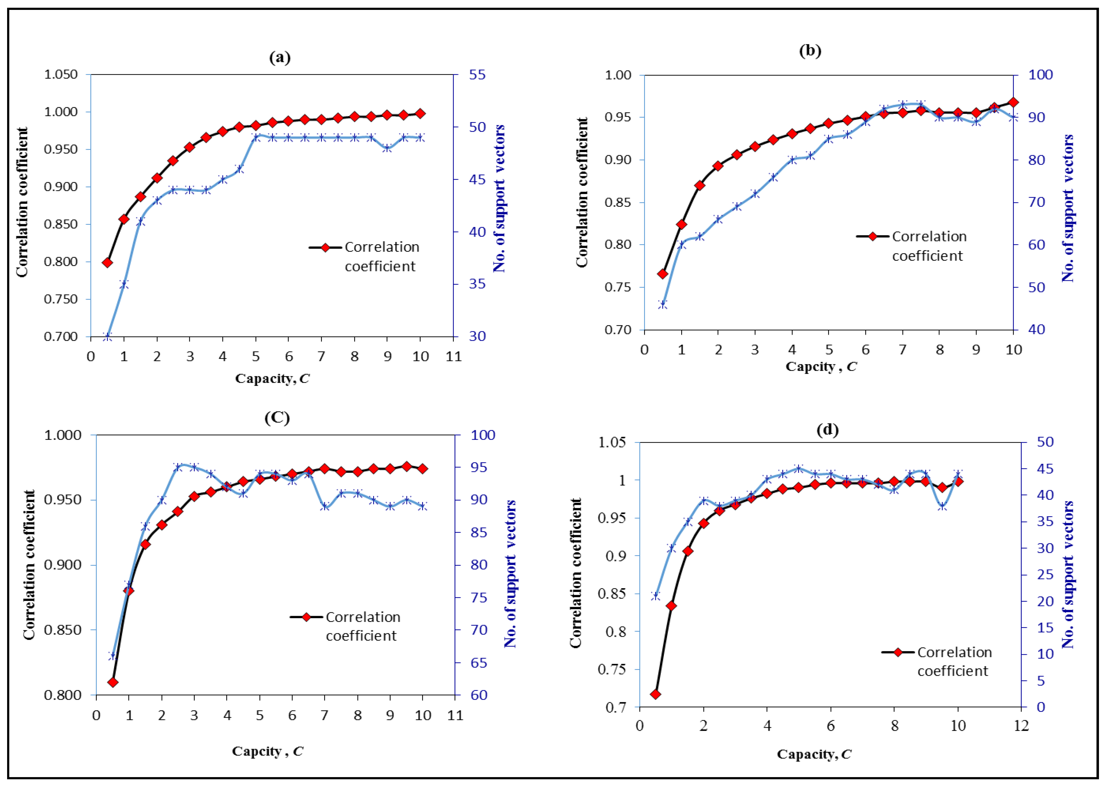
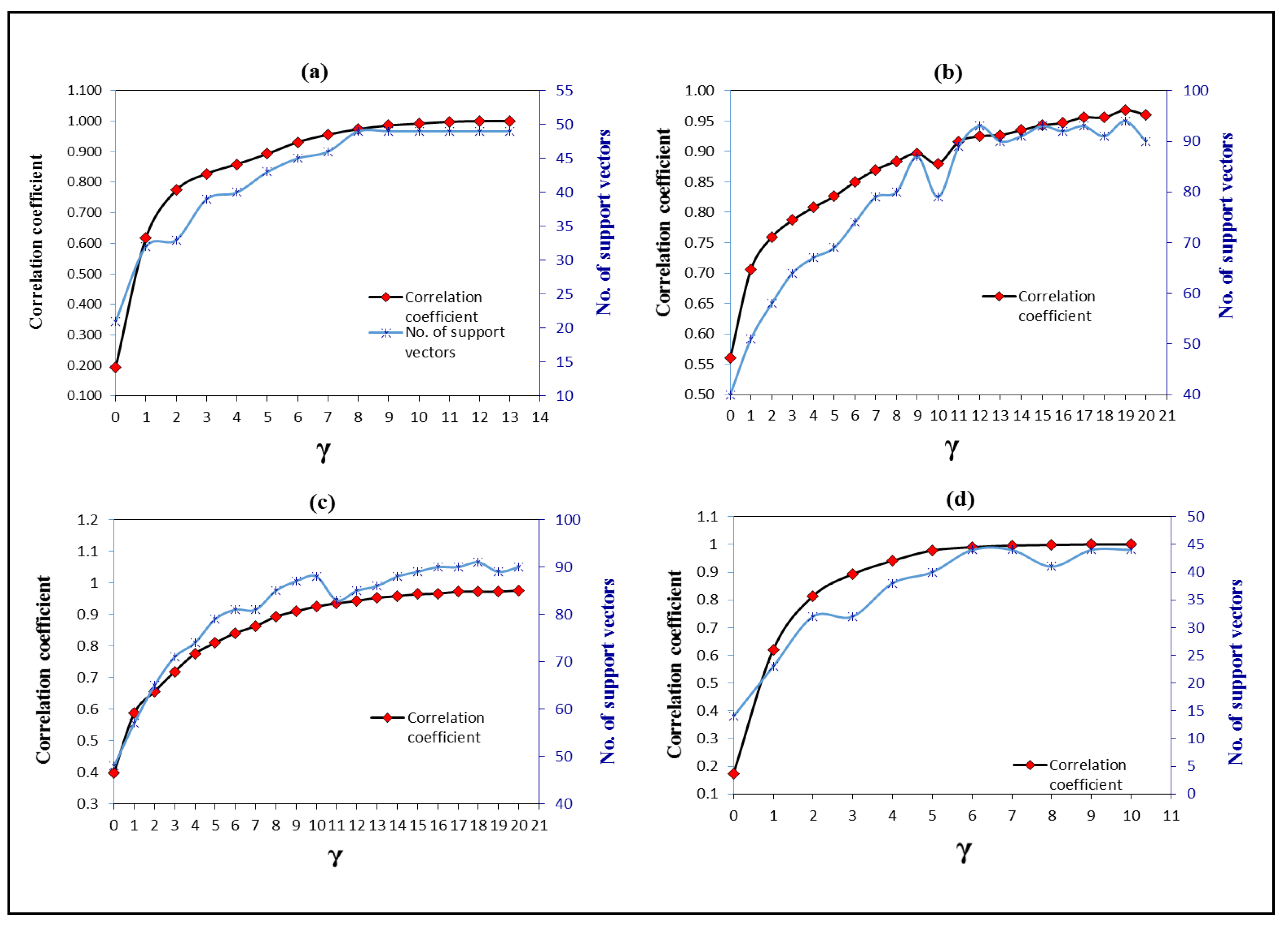
In the present study, the objective is to ascertain the appropriate values of the parameters γ and C. The replication processes that involved a number of parameters were also considered as the highlights of SVM and regarded as a key step in behaviour prediction model. At the initial stage of building the recommended model and throughout the training session of the input-output data, a constant value of γ equal to 0.1 was considered, while the values of C were changeable and in the range of 0 and 10. As a result, the prediction error was calculated as MSE, while correlation coefficient was computed as the number of the support vectors. Figure 3 illustrates that an increase in the used value of C leads to a small decrease in the value of MSE and in the number of the support vectors but, in contrast, causes an increase in the value of correlation coefficient. Furthermore, by keeping the emphasis of the observation on the parameter C, it was found that the highest correlation coefficient value was 0.998 and the lowest value of MSE point was 0.001. According to the observation, with an increase in the value of parameter C, there is a marginal reduction in the value of MSE, and then it shows an upward trend after the value of C reaches the optimal point. Therefore, it is advantageous to choose the parameter C to be 8.5 for station 4, and the remaining figures for every other station. In reality, it is important to first ascertain the applicable values for the hyper parameters C and γ because it will be a significant step in the implementation of any SVM model. Hence, conducting a trial and error procedure is important and necessary. The generalised accuracy has been assessed using different values of kernel hyper in relation to this context. Due to the shortcoming of parameter γ, it was resolved that its optimal value will be searched so that it is within the range of [0.001, 10] at increments of 1 for γ, while the values are fixed for C (C = 8.5) and Nu (Nu = 0.3). As a consequence, the optimal selection value of γ is derived using 10-fold cross-validation that involves repetition of ten times with the purpose of improving the reliability of the model outcomes. The final architecture of the model in the competition during the training session is such that the parameters yield minimum errors during the course of validation. The relationship between correlation coefficient and γ is presented in Figure 4. The figure illustrates where the value of correlation coefficient begins to rise as the value of γ increases, and attains its peak value at 8 for station 4. Thereafter, the selection of values of parameters takes place that offers the minimum generalisation error. For the model in training and forecasting phase, the best outcome is taken into consideration when choosing γ = 8 with a satisfactory number of support vectors 41 for station 4, while the remaining figures are for other stations.

3.4. SVM Model Development

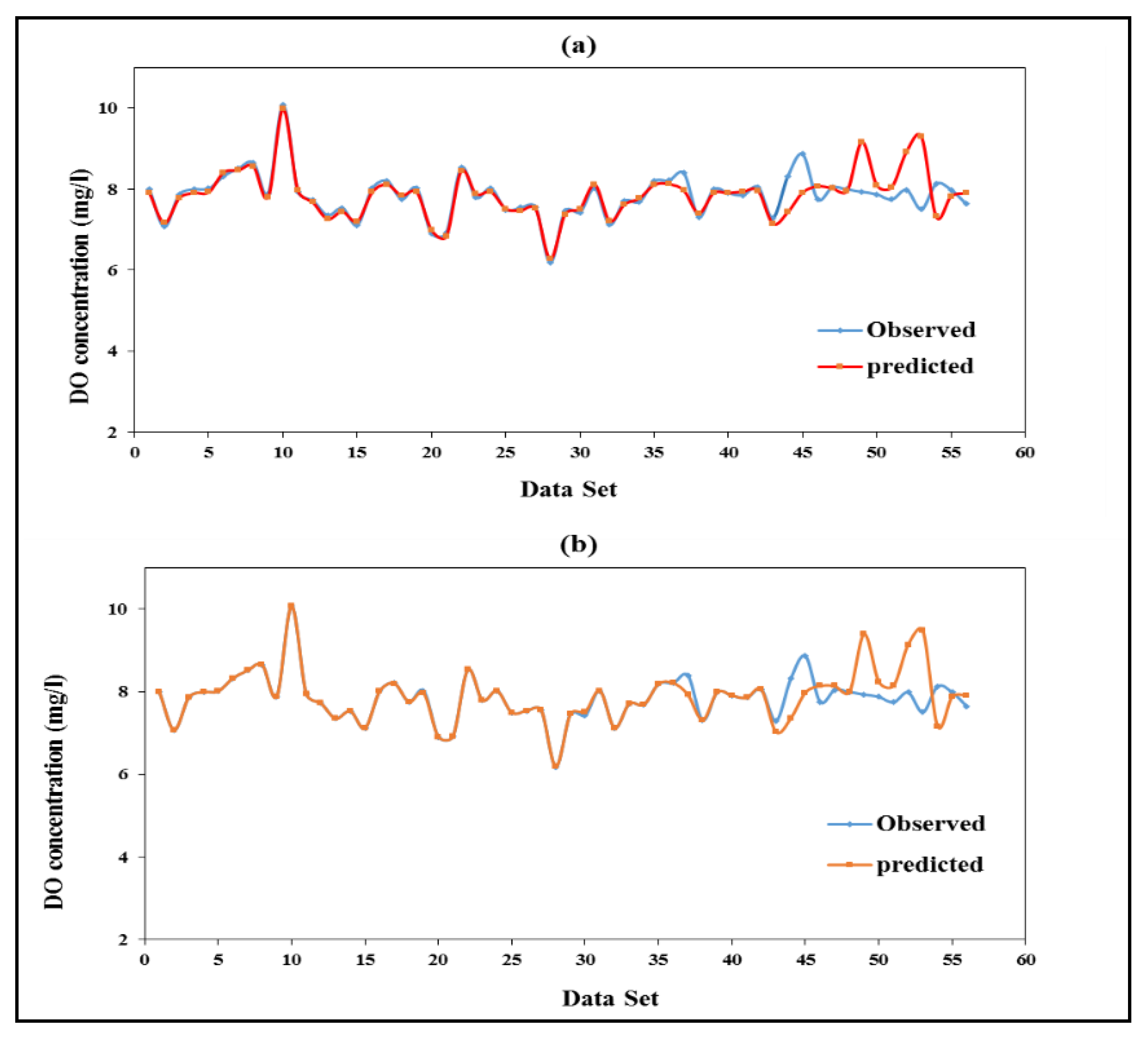
The cross validation procedure is regarded as one of the extensively used approaches for assessing the values of the model architecture parameters. The training dataset is unsystematically fragmented into a set number of V-folds (V1, V2, … Vn) so that the V-folds cross validation can be used. The chosen SVM model is then implemented in sequence as per the observations in relation to the V-1 folds. The expected results of the performing architecture can then be attained using the process with specific parameters on the sample V, so that the error defined by one of the statistical indices can be figured out. In other words, the sample or fold that was not visible during training of the SVM model was identified. The key limitation of this procedure is that the average accuracy for the v times causes a tendency for a consistent measure model error and impacts its stability, that is, the strength of the model for analysing the unseen session data. As shown in Table 5, the RMSE and MAE values attained by using the 10-fold cross-validation results in the best goodness of fit and performance. After the selection of the optimal kernel parameters, the Nu-RBF model is selected as the optimal model for evaluating the whole training data. Figure 5 presents a comparison of actual versus expected behaviour of DO concentration for testing data set at station 4: (a) Nu-SVM type model; (b) Epsilon-SVM type model. It can be seen that the both proposed model capable of predicting DO accurately but, in general, Nu-SVM outperformed Epsilon-SVM. While Figure 6 depicts the comparison between actual and predicted value of DO for all stations during testing.

3.5. Compression between Scenario One and Two

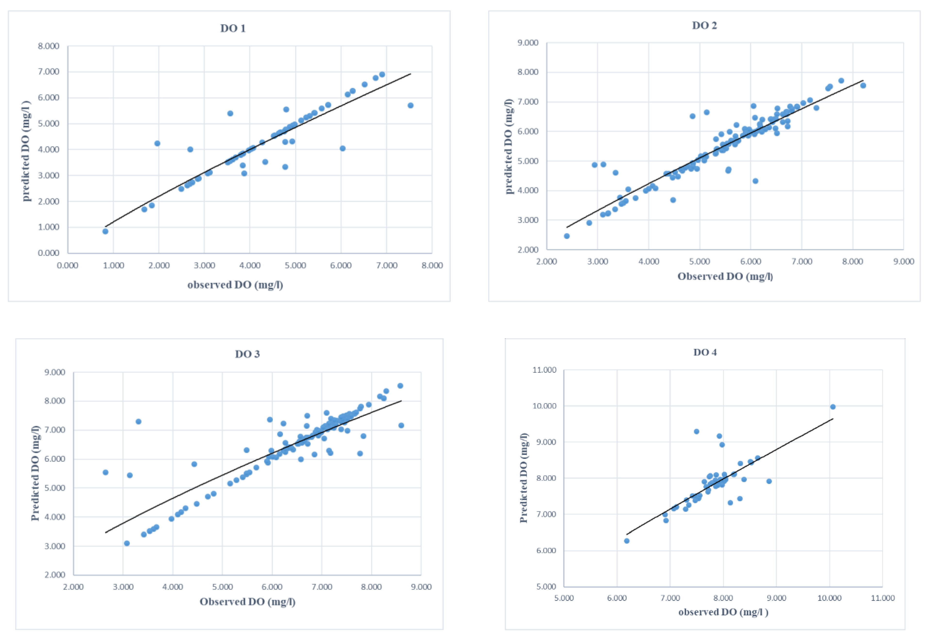
The compression between the two scenarios reveals that scenario 1 yields a more accurate result than scenario 2 in predicting DO in a two-week time horizon. Table 6 and Table 7 present the results. As observed in Table 6, the sensitivity analysis produces more accurate results when all the input parameters are included. In scenario 1, the best model is the first model, which produces the highest value for correlation coefficient equal to 0.99 while the lowest mean square error value is equal to 0.001 at station 4 after including all the six parameters as input to the model. Moreover, this model performed well in all stations where the mean square error is in the range of 0.001 to 0.44 and the correlation coefficient is in the range of 0.93 to 0.99 for all stations. Figure 7 presents a Scatter plot of the observed and expected values for Scenario 1 for all four stations. On the other hand, for scenario 2, most model proposed model performed poorly in predicting DO except the model where the predicted DO from all previous three stations were used as input to predict DO as station 4 which is considered as the best model that produces the highest value for correlation coefficient equal to 0.979. Table 8 depicts the performance of the proposed model in prediction DO in different horizon at all stations in terms of maximum residual error.

4. Conclusions

The prediction of water quality is very vital in monitoring the pollution and in sustaining the availability of potable water resources. Undoubtedly, it can afford early warnings when the water quality changes as well as it can reduce the adverse consequences resulting from the poor water quality. Herein, the SVM approach was introduced to estimate the water quality of Langat River Basin using six parameters. The presented model accurately estimated the water quality factors with relatively minor prediction errors, proving a quite efficient and robust performance. The model also can help in the optimization of water quality monitoring plans by decreasing the frequency, quantity of sampling sites, and water quality factors. Prediction precision with the maximum error was equal to 1% and CC was equal to 0.9987. Even though the outcomes seem to be reasonable, the application of water quality parameters is quite sensitive to the error level. 1% as a maximum error is comparatively on the higher side in such an application which triggers the need to improve it. In this regard, it is suggested to deploy the optimal kernel parameters determined and choose the Nu-RBF model as the optimal model.

Author Contributions

Formal analysis, A.S.A.Y., A.N.A., H.A.A., C.M.F. and A.E.; Methodology, A.S.A.Y., A.N.A., H.A.A., M.S.H. and M.E.; Writing—original draft, F.B.O., R.K.I. and A.E.; Writing—review & editing, A.E.-S.

Funding

This research was funded by Innovation & Research Management Center (iRMC), Universiti Tenaga Nasional, Malaysia, Bold 2025 grant coded RJO 10436494 and J510050822 and funded by the University of Malaya grant coded UMRG RP025A-18SUS.

Acknowledgments

The authors appreciate so much the facilities support by the Civil Engineering Department, Faculty of Engineering, University of Malaya, Malaysia.

Conflicts of Interest

The authors declare no conflict of interest.

References

  1. Tarmizi, A.; Ahmed, A.N.; El-Shafie, A. Dissolved Oxygen Prediction Using Support Vector Machine in Terengganu River. Middle-East. J. Sci. Res. 2014, 21, 2182–2188. [Google Scholar]
  2. Behmel, S.; Damour, M.; Ludwig, R.; Rodriguez, M. Water quality monitoring strategies—A review and future perspectives. Sci. Total Environ. 2016, 571, 1312–1329. [Google Scholar] [CrossRef] [PubMed]
  3. Lumb, A.; Sharma, T.C.; Bibeault, J.-F. A Review of Genesis and Evolution of Water Quality Index (WQI) and Some Future Directions. Water Qual. Expo. Health 2011, 3, 11–24. [Google Scholar] [CrossRef]
  4. Najah, A.; El-Shafie, A.; Karim, O.A.; Jaafar, O. Integrated versus isolated scenario for prediction dissolved oxygen at progression of water quality monitoring stations. Hydrol. Earth Syst. Sci. Discuss. 2011, 8, 6069–6112. [Google Scholar] [CrossRef]
  5. Najah, A.; El-Shafie, A.; Karim, O.A.; El-Shafie, A.H. Performance of ANFIS versus MLP-NN dissolved oxygen prediction models in water quality monitoring. Environ. Sci. Pollut. Res. 2014, 21, 1658–1670. [Google Scholar] [CrossRef] [PubMed]
  6. Ahmed, A.N.; El-Shafie, A.; Karim, O.A.; El-Shafie, A.H. An augmented wavelet de-noising technique with neuro-fuzzy inference system for water quality prediction. Int. J. Innov. Comput. Inf. Control 2012, 8, 7055–7082. [Google Scholar]
  7. Yoon, H.; Kim, Y.; Ha, K.; Lee, S.-H.; Kim, G.-P. Comparative Evaluation of ANN- and SVM-Time Series Models for Predicting Freshwater-Saltwater Interface Fluctuations. Water 2017, 9, 323. [Google Scholar] [CrossRef]
  8. Wang, Y.; Wu, L.; Engel, B. Prediction of Sewage Treatment Cost in Rural Regions with Multivariate Adaptive Regression Splines. Water 2019, 11, 195. [Google Scholar] [CrossRef]
  9. Liu, C.; Hu, Y.; Yu, T.; Xu, Q.; Liu, C.; Li, X.; Shen, C. Optimizing the Water Treatment Design and Management of the Artificial Lake with Water Quality Modeling and Surrogate-Based Approach. Water 2019, 11, 391. [Google Scholar] [CrossRef]
  10. Elzwayie, A.; El-shafie, A.; Yaseen, Z.M.; Afan, H.A.; Allawi, M.F. RBFNN-based model for heavy metal prediction for different climatic and pollution conditions. Neural Comput. Appl. 2017, 28, 1–13. [Google Scholar] [CrossRef]
  11. El-Shafie, A.; Najah, A.; Alsulami, H.M.; Jahanbani, H. Optimized Neural Network Prediction Model for Potential Evapotranspiration Utilizing Ensemble Procedure. Water Resour. Manag. 2014, 28, 947–967. [Google Scholar] [CrossRef]
  12. Wang, K.; Wen, X.; Hou, D.; Tu, D.; Zhu, N.; Huang, P.; Zhang, G.; Zhang, H. Application of Least-Squares Support Vector Machines for Quantitative Evaluation of Known Contaminant in Water Distribution System Using Online Water Quality Parameters. Sensors 2018, 18, 938. [Google Scholar] [CrossRef] [PubMed]
  13. Chang, M.-J.; Chang, H.-K.; Chen, Y.-C.; Lin, G.-F.; Chen, P.-A.; Lai, J.-S.; Tan, Y.-C. A Support Vector Machine Forecasting Model for Typhoon Flood Inundation Mapping and Early Flood Warning Systems. Water 2018, 10, 1734. [Google Scholar] [CrossRef]
  14. Wang, Z.; Liu, J.; Li, J.; Zhang, D.D. Multi-Spectral Water Index (MuWI): A Native 10-m Multi-Spectral Water Index for Accurate Water Mapping on Sentinel-2. Remote Sens. 2018, 10, 1643. [Google Scholar] [CrossRef]
  15. Yan, J.; Xu, Z.; Yu, Y.; Xu, H.; Gao, K. Application of a Hybrid Optimized BP Network Model to Estimate Water Quality Parameters of Beihai Lake in Beijing. Appl. Sci. 2019, 9, 1863. [Google Scholar] [CrossRef]
  16. Chen, Y.F. Influence and control strategies of agricultural nonpoint source pollution on water quality. China Resour. Compr. Utilization 2016, 34, 54–56. [Google Scholar]
  17. Akoteyon, I.S.; Omotayo, A.O.; Soladoye, O.; Olaoye, H.O. Determination of water quality index and suitability of urban river for municipal water supply in Lagos-Nigeria. Eur. J. Sci. Res. 2011, 54, 263–271. [Google Scholar]
  18. Malaysia.Jabatan Alam Sekitar. Malaysia Environmental Quality Report 2007; Department of Enviroment: Petaling Jaya, Malaysia, 2008; 84p, ISBN 9770127643008.
  19. River Water Quality (RWQ) | Malaysia Environmental Performance Index. Available online: http://www.epi.utm.my/v4/?page_id=102 (accessed on 5 April 2019).
  20. Heng, L.Y.; Abdullah, M.P.; Yi, C.S.; Mokhtar, M.; Ahmad, R. Development of Possible Indicators for Sewage Pollution for the Assessment Of Langat River Ecosystem Health. Malays. J. Anal. Sci. 2006, 10, 15–26. [Google Scholar]
  21. Aljanabi, Q.A.; Chik, Z.; Allawi, M.F.; El-Shafie, A.H.; Ahmed, A.N.; El-Shafie, A. Support vector regression-based model for prediction of behavior stone column parameters in soft clay under highway embankment. Neural Comput. Appl. 2018, 30, 1–11. [Google Scholar] [CrossRef]
  22. Afiq, H.; Ahmed, E.; Ali, N.; Othman, A.; Aini, K.; Mukhlisi, H.M. Daily forecasting of dam water levels: Comparing a support vector machine (SVM) model with adaptive neuro fuzzy inference system (ANFIS). Water Resour. Manag. 2013, 27, 3803–3823. [Google Scholar] [CrossRef]
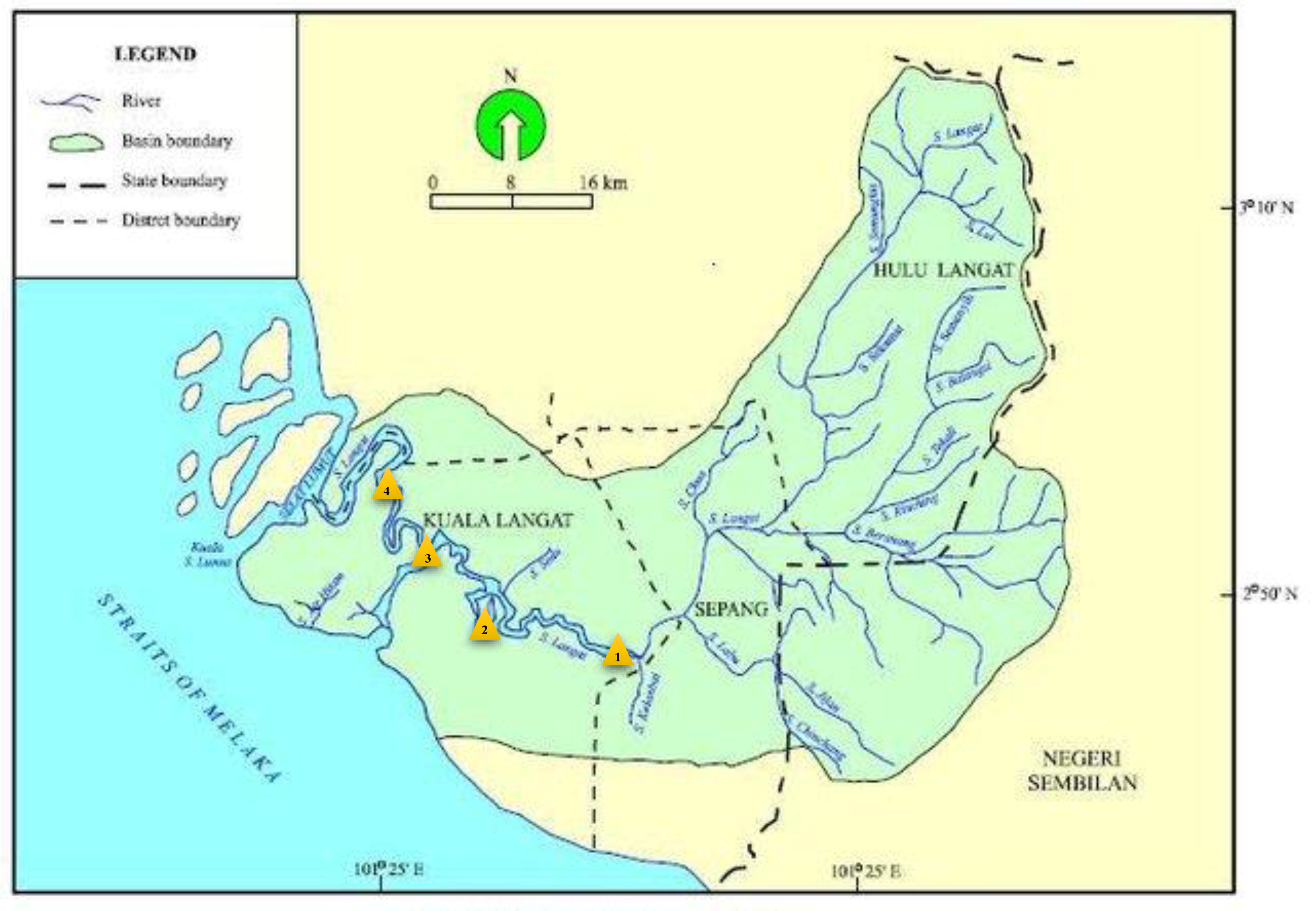
Figure 1. Water station on Langat River basin map.
Water 11 01231 g001
Figure 2. Hyperplane and the basic concept of support vector machine (SVM) [21].
Water 11 01231 g002
Figure 3. The result of various capacity parameter C, of SVM model, for (a) station 1; (b) station 2; (c) station 3; and (d) station 4.
Water 11 01231 g003
Figure 4. The result of various capacity parameter Gamma, of SVM for (a) station 1; (b) station 2; (c) station 3; and (d) station 4.
Water 11 01231 g004
Figure 5. Comparison of actual versus predicted behavior Dissolved Oxygen (DO) concentration: (a) Nu-SVM type model and (b) Epsilon-SVM type model.
Water 11 01231 g005
Figure 6. Comparison between actual and predicted value for DO.
Water 11 01231 g006aWater 11 01231 g006b
Figure 7. Scatter plots between the observed and predicted value for Scenario 1.
Water 11 01231 g007
Table 1. Basic statistics of the measured water quality parameter in Langat River.
Sampling SiteBasic StatisticDO (mg/L)BOD (mg/L)COD (mg/L)pHSS (mg/L)AN (mg/L)
Station 1Mean4.346.2929.776.46160.450.59
Min0.83142.410.10.01
Max7.5323997.3610501.69
SD1.3544.69117.070.691990.443
CV31.274.557.310.612474.9
Station 2Mean4.345.7725.546.58121.30.96
Min0.87173.810.01
Max7.524707.928213.73
SD1.113.5912.740.70116.580.662
CV25.6762.2549.9010.7096.1169.23
Station 3Mean5.815.2923.727.01182.91.11
Min3.55126.1050.01
Max7.6217668.2814005.75
SD0.772.5011.870.323202.940.995
CV13.247.3450.064.61110.9690.01
Station 4Mean5.508.0330.507.07272.441.56
Min2.39255.8430.01
Max8.22784.107.9119106.65
SD1.194.8415.240.29350.521.27
CV21.6560.2949.94.20128.6681.44
Table 2. Performance of SVM model with four kernel function.
Kernel FunctionMean Squared Error Correlation Coefficient
TrainingTestingTrainingTesting
Linear0.2290.1890.5640.438
Polynomial0.1770.2170.7320.496
RBF0.1770.3220.9980.801
Sigmoid155.886418.7350.1050.336
Table 3. The result of various Epsilon parameter ε, of SVM model where C = 8.5 and gamma = 0.2 of total behavior prediction model.
εMean Error SquaredCorrelation CoefficientNo. of Support Vectors
(Train)(Test)(Train)(Test)(Overall)
0.0010.0080.3050.9760.2860.78536
0.10.0300.3530.9100.1980.70327
0.20.0740.2260.8020.1660.65414
0.30.1180.2120.6880.1300.5679
0.40.1440.2220.6330.1260.5196
0.50.2060.2750.5380.1040.4435
Table 4. Nu-RBF performance utilizing different values of Nu with fixed (gamma = 8, capacity = 8.5) of Total behavior prediction model.
NuMean Error SquaredCorrelation CoefficientNo. of Support Vectors
(Train)(Test)(Train)(Test)(Overall)
0.0010.3570.3630.4160.0570.3392
0.10.0180.3400.9460.2410.74333
0.20.0030.3020.9920.3060.80241
0.30.0010.3260.9980.2720.79741
0.40.0010.3210.9980.2780.80144
0.50.0010.3310.9980.2680.79542
Table 5. Statistical evaluation using 3, 5, 7, 10, and 15-fold cross-validation for Epsilon-RBF and Nu-RBF models.
Statistical EvaluationV-Fold
3571015
ε-RBF Model:
RMSE0.4580.1640.1670.1640.164
MAE0.3930.5380.5300.5380.538
CR0.60500.9330.9330.9330.933
Nu-RBF model:
RMSE0.0890.0700.0890.0890.077
MAE0.6480.6460.6460.6480.632
CR0.9800.9860.9800.9860.984
Table 6. Correlation coefficient for Scenario 1.
ModelInput ParametersCorrelation CoefficientMean Square Error
DO 1DO 2DO 3DO 4DO 1DO 2DO 3DO 4
1DO, BOD, COD, SS, pH, AN0.990.990.930.950.0040.0440.0350.001
2DO, BOD, COD, SS, pH0.920.850.640.720.1410.2810.2120.008
3DO, BOD, COD, SS, AN0.900.820.820.730.1750.1310.2030.071
4DO, BOD, COD, pH, AN0.970.940.880.920.0580.0840.0520.009
5DO, BOD, SS, pH, AN0.950.910.830.850.0810.1240.1050.040
6DO, COD, SS, pH, AN0.960.920.790.820.0680.1600.1350.038
Table 7. Results for scenario 2.
ModelInput ParametersCC
DO 2DO 3DO 4
1DO 10.279
2DO 1 0.236
3DO 2 0.258
4DO 1, DO2 0.571
5DO 1 0.503
6DO 2 0.344
7DO 3 0.361
8DO 1, DO2 0.746
9DO 1, DO3 0.656
10DO 2, DO3 0.701
11DO 1, DO2, DO 3 0.979
Table 8. Maximum residual error for DO.
StationMaximum Residual Error
1 Week2 WeeksMonth
12.2642.0681.409
21.9240.6340.525
33.9923.042.559
40.9941.1290.450