Evaluation of Distribution Properties of Non-Point Source Pollution in a Subtropical Monsoon Watershed by a Hydrological Model with a Modified Runoff Module

Abstract

Non-point source pollution (NPS) is difficult to manage for watersheds, due to the scattering of pollution sources and uncertainty over the time it takes to accumulate. Since local agriculture and poultry rearing prevail, NPS occupies a large proportion of local pollution. In this paper, we modified the runoff module of the Soil and Water Assessment Tool (SWAT) to study the distribution properties and the effect of control of NPS in the Binjiang watershed in Southern China. The model was run from 2005 to 2014. The runoff simulation’s accuracy had apparently improved compared to the original model, as the Nash coefficient (Ens) had improved from 0.72 to 0.89, and the determination coefficient (R²) had improved from 0.75 to 0.91, an improvement in accuracy of 23.61% (Ens) and 21.33% (R²). Thus, the modified model (SWAT-m) is more adaptable for the simulation of extensive non-urban watersheds in subtropical monsoon climates. The validated model was used in further analysis. The results show that 82–90% of total nitrogen and 83–89% of total phosphorus were concentrated in the period from April to September annually. Through the introduction of the pollution generation potential parameter Φ_i, we obtained the descending order of all sub-basins in terms of their pollution generation potential. The critical source areas (CSAs) were found to be the northeast sub-basins in lower terrain that is used mainly for agricultural applications, accounting for 53% of the total watershed. The accumulation time is April to July, occupying 69% of annual generation. The simulation of management measures showed that NPS control has a good effect, with a 15 m filter strip in CSAs. Ammonia nitrogen and total phosphorus can be reduced apparently by 32% and 43%, respectively. The results may provide support for the management of NPS in watersheds under similar conditions.

1. Introduction

The Binjiang watershed, located in Qingyuan City, Guangdong Province, China, is an important source of local water supply for agriculture. It covers the area of latitude 23°44′30” N–24°16′04” N, longitude 112°32′40” E–113°4′50” E, as illustrated in Figure 1. Since local agriculture and poultry rearing prevail and there is abundant precipitation from the subtropical monsoon climate, non-point source pollution (NPS) occupies a large proportion of local water pollution. NPS is a form of pollutant that flows into underground or surface water from dispersed, wide-ranging, and traceable sources [1]. Compared to point-source pollution, NPS has more a complex composition of pollutants, a larger range of distribution, and more uncertain transmission paths. The distribution properties of NPS are important for NPS control and management.

The NPS model is an extended hydrological model that includes additional modules for assessing the release, migration, and leakage of pollutants from land sources, soil erosion, and sediment transport [2]. Rapid advances in remote sensing and geographical information systems (GISs) during the past three decades have provided an enormous number of opportunities for hydrology research [3]. The GIS-based distributed hydrological model Soil and Water Assessment Tool (SWAT) was developed by the USDA (United States Department of Agriculture), and is currently being utilized in several large basin projects, such as the HUMUS (Hydrologic Unit Model of the United States) project [4]. This model is also used as a decision tool [5] to predict NPS pollution load [6] and for the assessment [7] of NPS pollution reduction effects of various control measures [8]. Through the combined use [9] of land use changes [10] and climate changes [11], it is also used to predict the impact of future climate/land use scenarios [12] on hydrology [13] and pollution in basins [14]. However, researchers have usually focused on the total outflow load or concentration per hectare of NPS rather than the NPS’s properties, such as the generation potential. Nevertheless, the runoff module of the original SWAT has some limitations. Several researchers have found that the simplification of the surface runoff equation of SWAT does not comply with real runoff generation under certain conditions [15,16]. Therefore, we modified the surface-runoff module of SWAT, and the modified SWAT-m model was applied to do this research. As for the NPS outflow load per unit area, it is difficult to tell whether a certain amount, say 1 t/ha annually, is high or low, as this depends on local pollution or different precipitation conditions. The only standard of a certain outflow load per hectare could be a violation of justice when deciding on the NPS critical source areas (CSAs). Thus, we introduced a new dimensionless parameter Φ_i to measure the NPS generation potential of each sub-basin impartially. Through this, we can compare the NPS contribution of different sub-basins and pollutant components under various circumstances and, therefore, accurately position NPS CSAs.

Through the combination of remote sensing and GIS, we established this model to study the hydrology and NPS in a subtropical monsoon watershed. Further study of NPS, especially the distribution properties of NPS outflow and generation, the accurate positioning of NPS CSAs, and the impact of different filter strips on NPS pollutants, will contribute to NPS control and management in watersheds under similar conditions.

2. Model and Methods

2.1. The Modification of the Hydrological Model

The distributed hydrological model Soil and Water Assessment Tool (SWAT) has a modular structure and consists of hydrology, sediment, and chemical subroutines applicable to watershed scales. The hybrid model is spatially based on hydrological response units that include both physical and conceptual methods [17]. The hydrologic cycle as simulated by SWAT is based on the water balance equation [18]. The in-stream kinetics used in SWAT for nutrient/pollutant routing are adapted from a widely used stream water quality model, QUAL2E [19]. In this study, nitrogen and phosphorus are the main nutrients/pollutants.

Surface runoff is flow that occurs along a sloping surface. In the runoff module of SWAT, the surface runoff volume is computed using a modification of the Soil Conservation Service (SCS) curve number method [20]. The equation for the SCS curve number method is as follows:

$$Q_{\mathit{surf}}=\frac{{\left(R_{\mathit{day}}{-I}_a\right)}^2}{R_{\mathit{day}}{-I}_a+S}$$

(1)

where Q_surf is the accumulated runoff or rainfall excess (mm), R_day is the rainfall depth for the day (mm), I_a are the initial abstractions, which include surface storage, interception, and infiltration prior to runoff (mm), and S is the retention parameter (mm). The retention parameter varies spatially due to changes in soils, land use, management, and slope and temporally due to changes in soil water content. The retention parameter S is defined as:

$$\mathrm{S}=25.4\left(\frac{1000}{\mathit{CN}}-10\right)$$

(2)

where CN is the curve number for the day. The initial abstractions, I_a, are commonly approximated as 0.2S in SWAT, which is the limitation of this module. In the original equation, the relation between I_a and S is described by another parameter λ. Here, λ is fixed at 0.2, where we would modify the module.

S = λ I_a

(3)

Many researchers have proved that the fixed initial abstraction 0.2 does not match well with their study area. Researchers have taken measures to find out that the initial abstraction λ ranges from 0 to 0.3 [15,16,20]. Woodward [21] also proved by his research that, in the experience of almost 90% of researchers, λ should be less than 0.2. In order to avoid deviation in the simulation caused by a single initial abstraction, this paper adopts the method of a segmentation value to improve the model, that is, a different initial abstraction λ is adopted according to the curve number (CN) value ranges of different regions. Based on data about local precipitation and hydrology events, we have obtained the initial abstraction values under different conditions through the event analysis and back calculation method. For instance, for an area covered by a natural forest with sandy-loam soil, the CN value is about 50–65, and the corresponding initial abstraction is relatively high: λ is about 0.12. For a concentrated residential area with clay soil, the CN values are relatively high, approximately 85–95, and the initial abstraction is relatively low: about 0.05. For cross-sectional conditions, such as clay soil farmland, the CN value is between 65 and 85, and the corresponding initial abstraction is around 0.08. According to the above classification method, we used Equation (1) to obtain the flow equation as follows:

$$Q_{\mathit{surf}}=\{ \begin{array}{l}\frac{{\left(R_{\mathit{day}}-005S\right)}^2}{\left(R_{\mathit{day}}+0.95S\right)}\hspace{1em}\hspace{1em}\hspace{1em}\left(\mathit{CN} \ge 85\right)\\ \frac{{\left(R_{\mathit{day}}-0.08S\right)}^2}{\left(R_{\mathit{day}}+0.92S\right)} \hspace{1em}\hspace{1em}\left(85 \ge \mathit{CN} \ge 65\right)\\ \frac{{\left(R_{\mathit{day}}-0.12S\right)}^2}{\left(R_{\mathit{day}}+0.88S\right)}\hspace{1em}\hspace{1em}\hspace{1em}\left(65 \ge \mathit{CN}\right)\end{array}.$$

(4)

Through the modification of the surf.f, main.f, and simulate.f functions from the source code of SWAT in Visual Studio, we recompiled the modified code into the swatuser.exe program for further simulation and research. The modified version of SWAT is denoted SWAT-m. We compare the modified model with the original model in the next section.

2.2. Establishment of Databases

Spatial and attribute databases were established to build up the model. The databases include topography, land cover, soil classification, and weather data.

Firstly, topography data were extracted from a digital elevation model (DEM). The data used in this study is from the International Scientific Data Service Platform [22]. We performed slope classification and hydrological analysis based on the DEM.

Secondly, we used as a source of land cover condition data the National Earth System Science Data Sharing Infrastructure [23]. The classification of land use conditions in the study area is shown in

Table 1. The classification of land use conditions of the study area.

Classification	Land Use Code	Area (km2)	Percentage (%)	Details
Waters	WATR	19.76	1.16	streams and lakes
Forest	FRST	1145.8	67.14	natural and artificial forest
Pasture	PAST	101.44	5.94	shrub and herbaceous plants
Farmland	AGRL	260.57	15.27	cropland, rice paddies, and other farming activities
Resident	URBN	68.25	4.01	human residents
Agriculture	UINS	110.67	6.49	sparse woods, livestock, poultry breeding, and others

.

Thirdly, the soil classification and soil properties were extracted from the 1:500,000 scale FAO-UNESCO (Food and Agriculture Organization of the United Nations) Digital Soil Map of the new comprehensive Harmonized World Soil Database, as shown in Figure 2. Most of the soil properties that were obtained refer to “Guangdong soil” [24] and Soil Science, Chinese Academy of Science [25]. Additionally, daily weather data from six stations in the watershed from 2005 to 2014 were obtained from the China Meteorological Science Data Sharing Service Network [26], which is shown in Figure 3.

The remaining data, such as point source, agricultural, and water supply volume data, were extracted from local chronicles and environmental survey reports from the local Environmental Protection Agency. According to the input data requirements, all geographical coordinates of spatial data need to be unified. In this study, the projection coordinate system used was Gauss Kruger Projection from the Beijing 54 Coordinate System.

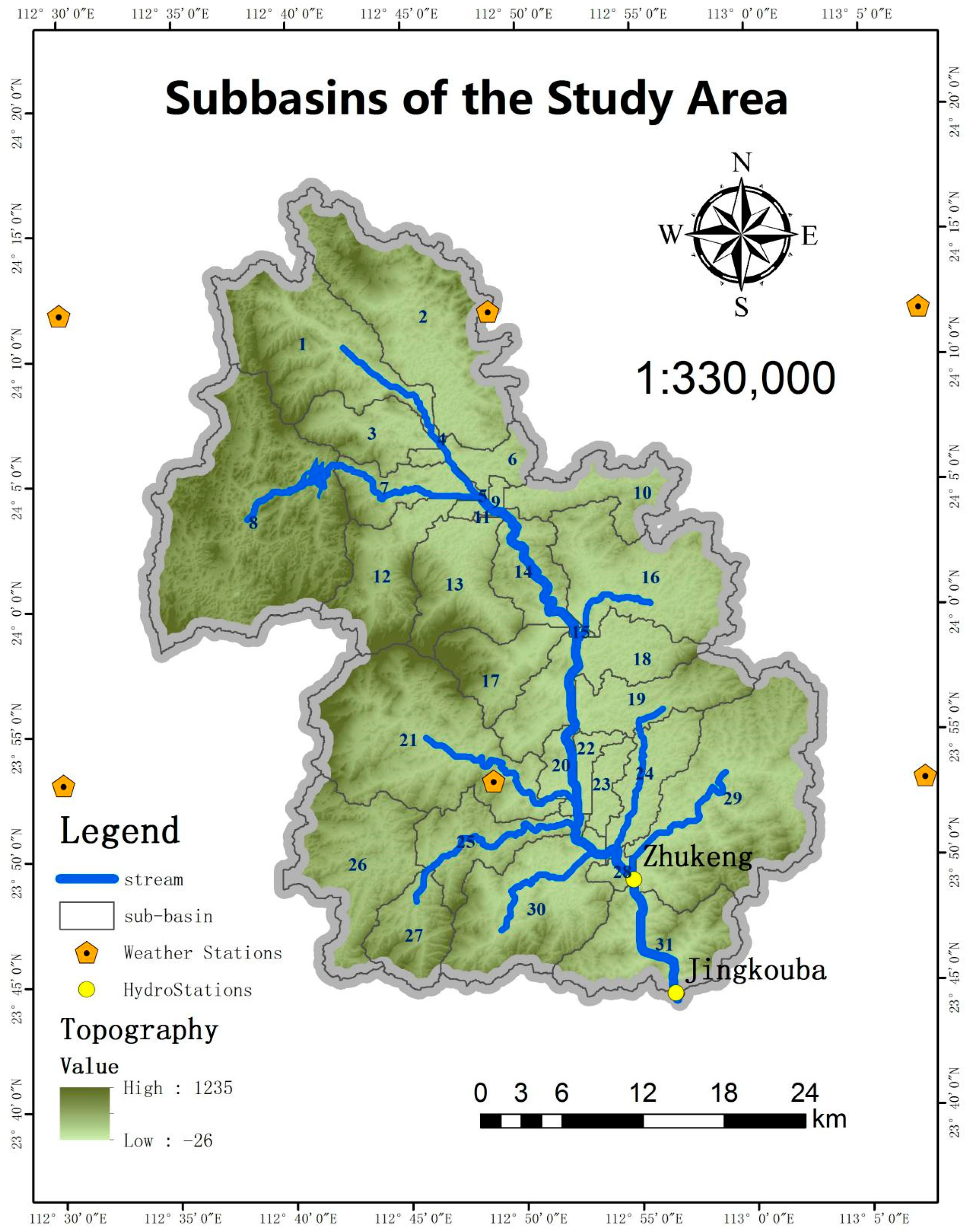
2.3. Delineation of Sub-Basins and the Hydrologic Response Unit

To simulate runoff in a watershed with a river network, we should first delineate its sub-basins. The model obtains the flow direction of each grid by the maximum gradient method, with the D8 algorithm, on the DEM, and then counts the number of flows through the grid to estimate the cumulative flow [27]. Through the process of water delineation, the study area is divided into 31 sub-basins, which are shown in Figure 3.

Based on the division of the study area into sub-basins, the model applies an algebra calculation to the land use layer, the soil classification, and the slope classification to generate the smallest hydrological response unit (HRU). The slope classification refers to cultivated land gradients: less than 15 degrees; 15–25 degrees; and greater than 25 degrees. According to the local conditions, the multiple HRU threshold of land use, slope gradient, and soil classification was set to 20%, 20%, and 10%, respectively. After the raster calculation, 749 HRUs were generated in the study region. Runoff was predicted separately for each HRU and routed to obtain the total runoff for the watershed. Now, we are ready to run the model.

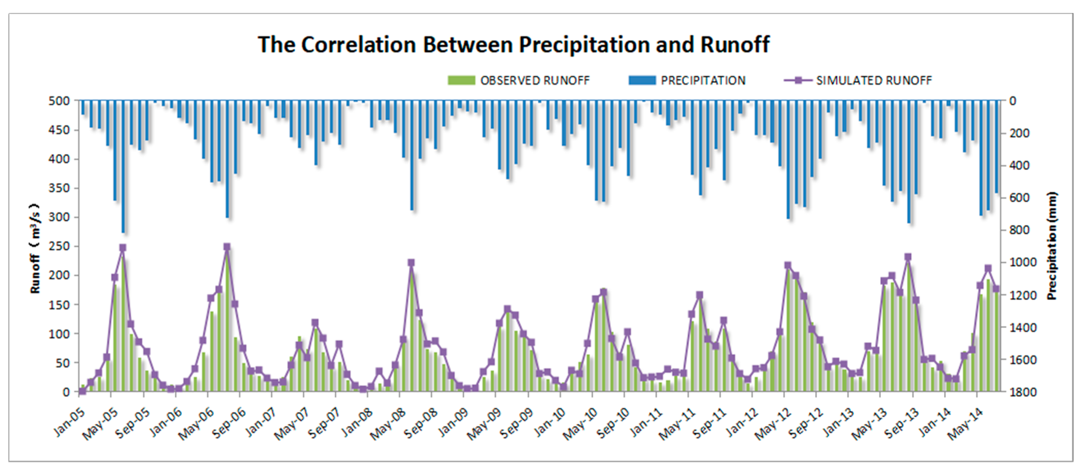
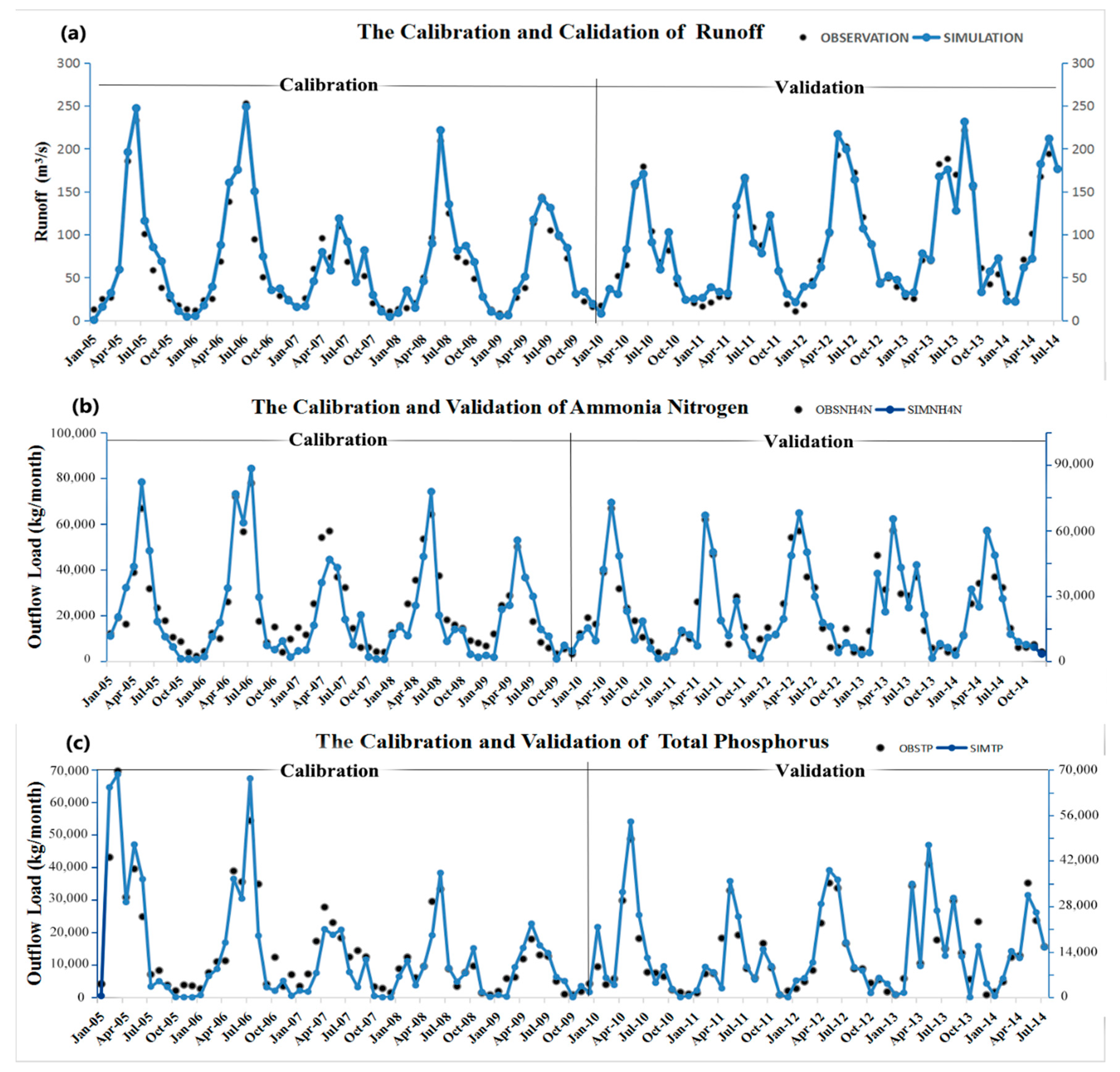
2.4. Calibration and Validation

In this study, the model was calibrated by the SUFI-2 algorithm method through the model SWAT-CUP. The measured data from 2005 to 2009 were used to calibrate the parameters, and the data from 2010 to 2014 were used to validate the model. To evaluate the simulation’s accuracy, we applied three indicators: determination coefficient (R²), relative error (Re), and Nash coefficient (Ens) [28,29].

2.5. The NPS Generation Potential Parameter

Because the specific value of the outflow load per hectare of NPS is impacted by various kinds of pollutants, the overall pollution levels, and the precipitation conditions in different regions, the only standard of a certain load per hectare could be a violation of justice in an NPS comparison between different districts and various pollutants and when deciding on NPS CSAs. For instance, with the standard of 10kg/ha for NPS CSAs, for some upstream watersheds, maybe only one sub-basin is identified as a CSA, yet for some downstream populated watersheds, maybe all sub-basins are over 10kg/ha and thus constitute CSAs under this criteria, which is improper for CSAs and NPS management. In order to analyze and compare the generation potential of NPS among different regions and facilitate the accurate positioning of NPS CSAs, we introduce a new dimensionless parameter to measure the generation potential of NPS in each sub-basin. The equation is as follows:

$${\Phi }_i=\frac{C_i\times A}{{\displaystyle \sum _{i=1}^n}(C_i\times A_i)}$$

(5)

where Φ_i is the generation potential parameter of sub-basin No. i of a certain kind of NPS pollution; i stands for the number of the sub-basin, n is the total number of sub-basins in the study area; C_i stands for the average pollutant yield per unit area in the time step, kg/ha monthly or annually; A_i stands for the area of sub-basin No. i; and A stands for the total area of all sub-basins. Φ_i = 1 is the average level of NPS generation, which means that all sub-basins have the same generation potential of a certain pollutant. The lower the contribution is, the closer the value of Φ_i is to zero; conversely, the higher the generation potential is, the higher the value of Φ_i is; the maximum is less than n. For different kinds of pollutants, the value of Φ_i can be added to show the multiple contributions of a certain sub-basin.

2.6. The Theory of Filter Strips for NPS Control

After obtaining the distribution properties of NPS CSAs, this section focuses on pollution control in those CSAs, mainly sub-basins 1–11 upstream in the watershed. Among the control measures in the Best Management Practices (BMPs), such as Terracing, Contouring, Filter Strips, and Artificial Wetlands [7], we chose filter strips, as the NPS control effect is ideal and the construction and operation cost is relatively low, especially in rural areas [8].

A filter strip is a plant-intensive strip that intercepts and filters runoff from an uphill or upstream area. It can decrease the flow rate and increase the infiltration of the area to reduce runoff and pollutants. The filter strip algorithm that SWAT uses is derived from White and Arnold’s research methods for vegetation filter strips, which can effectively reduce sediment, pollutants, bacteria, and pesticide components, but do not affect runoff [18,30]. A filter strip’s trapping of sediments and nutrients in the SWAT management module is calculated as:

$$Tra{p}_{ef}=0.367\times {\left(Widt{h}_{filstrip}\right)}^{0.2967}$$

(6)

$$Tra{p}_{ef,sub}=\frac{\left(2.1661\times Widt{h}_{filstrip}-5.1302\right)}{100}$$

(7)

where Trap_ef and Trap_ef,sub are the surface and subsurface flow constituent loadings that the filter strip traps, respectively, and Width_filstrip is the width of the filter strip. The proper parameter of the filter strip’s width can be found in FILTERW.mgt in the management module of SWAT. Based on the hydro-geological conditions, we present a better design of a riparian filter strip through a scenario simulation of a filter strip with a width of 3–30 m, and provide a reference for NPS control in similar clay-loam areas in a subtropical monsoon climate.

3. Results and Discussion

3.1. Results of Simulations with the Model

3.1.1. Parameter Sensitivity Analysis

In this study, the model was calibrated using the SUFI-2 algorithm method through the model SWAT-CUP. The first 12 sensitive parameters of runoff were obtained through a sensitivity analysis and are shown in

Table 2. The sensitive parameters for the runoff simulation.

No	Parameter	File	p-Value	t-Stat	Details
1	ALPHA_BF	gw	0.00	7.50	Base flow division coefficient
2	CH_K2	rte	0.01	−3.45	River effective hydraulic conductivity coefficient
3	CANMIX	hru	0.03	2.35	Canopy maximum water storage coefficient
4	CH_N2	rte	0.11	−1.65	Main channel Manning coefficient
5	GW_DELAY	gw	0.23	1.24	Ground water delay coefficient
6	BIOMIX	mgt	0.26	−1.20	Biomass mixing efficiency
7	GWQMN	gw	0.31	1.00	Threshold depth of a shallow water aquifer required for return flow to occur (mm)
8	CN2	mgt	0.47	−0.75	SCS runoff curve number
9	ESCO	hru	0.61	−0.55	Soil evaporation compensation coefficient
10	SURLAG	bsn	0.78	0.33	Surface runoff delay coefficient
11	GW_REVAP	gw	0.85	−0.17	Ground water “Revap” coefficient
12	EPCO	hru	0.97	−0.05	Plant uptake compensation factor.

. p-values were used to determine the significance of the sensitivity (values close to zero have more significance). t-Stat provides a measure of sensitivity (larger absolute values are more sensitive) [31].

As for the pollutants, the sensitivity analysis showed that five parameters (nitrate percolation coefficient, benthic source rate for NH₄-N, rate coefficient for organic N settling in the reach at 20 °C, rate constant for biological oxidation of NH₄ to NO₂, and rate constant for hydrolysis of organic N to NH₄) have a great influence on ammonia nitrogen. The phosphorus absorption coefficient, soil phosphorus separation coefficient, phosphorus permeability coefficient, residual mineralization rate, and rate constant for organic phosphorus transferred to dissolved phosphorus at 20 °C have a great influence on total phosphorus. These parameters were applied in the calibration process.

3.1.2. The Comparison of SWAT and SWAT-m

In order to prove that the improved model has better adaptability, the original SWAT was applied to simulate runoff in the same area as a blank control. The input data were all the same as the inputs into the modified model (SWAT-m). The best parameters of the calibration period (2005–2009) were applied to the validation period (2010–2014) for verification. The comparison of the runoff simulation accuracy of SWAT and SWAT-m based on three indicators (determination coefficient (R²), relative error (Re), and Nash coefficient (Ens)), is depicted in

Table 3. The comparison of SWAT and SWAT-m on the runoff simulation accuracy.

Accuracy Parameters	Calibration Period			Validation Period
	SWAT	SWAT-m	Improved Percentage	SWAT	SWAT-m	Improved Percentage
Ens	0.76	0.92	21.05%	0.72	0.89	23.61%
R2	0.82	0.94	14.63%	0.75	0.91	21.33%
Re	18%	10%	44.44%	27%	14%	48.15%

.

It can be seen from Table 3 that the R² of SWAT is 0.82 and 0.75 for the calibration period and the validation period, respectively, which is greater than the standard 0.60 [29]. The Nash coefficient (Ens) of the original SWAT is 0.76 and 0.72 for the calibration period and the validation period, respectively, which does not reach the standard of 0.75 [28]. These results indicate that the simulation results are not that ideal. Apparently, the simulation accuracy is not as good as SWAT-m, especially for the validation period. From the comparison of the Nash coefficients, the simulation accuracy of SWAT-m has improved by 23.61%. The improvement in simulation accuracy is more obvious in the comparison of relative error, which is as high as 27% in the validation period, and the simulation accuracy of SWAT-m has improved by 48.15%. Therefore, if the original model is used in further NPS simulation, the relative error generated by the runoff simulation will further increase; the principle is similar to the butterfly effect. In summary, the improved model (SWAT-m) has higher runoff simulation accuracy; thus, we will carry out NPS simulation using the modified model.

3.1.3. Results of Simulations with the Modified Model

The model was calibrated using observed values from 2005 to 2009 and with an optimal set of parameters. Results of Re < 10%, R² > 93%, and Ens > 91% were obtained. Then, we input the best parameters and reran the model over the validation period (2010–2014). The results of the simulation well-agreed with the observed values, with Re < 15%, R² > 89%, and Ens > 90%. The comparison of the simulated and measured values of runoff is shown in Figure 4a.

As for pollutants, after calibration and validation of the runoff simulation, SWAT-m was applied to a pollutants simulation in which the calibration and validation time was the same as in the runoff simulation. The comparison of the simulated and measured values of the monthly average ammonia nitrogen and total phosphorus load is shown in Figure 4b,c. The best calibration and validation results for ammonia nitrogen were Re = 38%, R² = 0.85, and Ens = 0.71 (calibration) and Re = 39%, R² = 0.77, and Ens = 0.69 (validation). For total phosphorus, the best calibration and validation results were Re = 30%, R² = 0.78, and Ens = 0.79 (calibration) and Re = 37%, R² = 0.75, and Ens = 0.72 (validation). Generally, if the absolute value of Re is less than 15%, the absolute value of R² is greater than 0.6, and the absolute value of Ens is greater than 0.75, the simulation result is sufficiently accurate [28]. The standard for nutrient assessment is not as high. The absolute value of relative error should be less than 40%, the absolute value of the Nash coefficient (Ens) should be greater than 0.5 [31], and the standard for R² is the same as that for runoff [32]. We can tell that the simulations for both nitrogen and phosphorus are able to comply with the standard of accuracy, indicating that the modified model is effective for further research in NPS simulation and analysis.

3.2. Temporal and Spatial Distribution of NPS

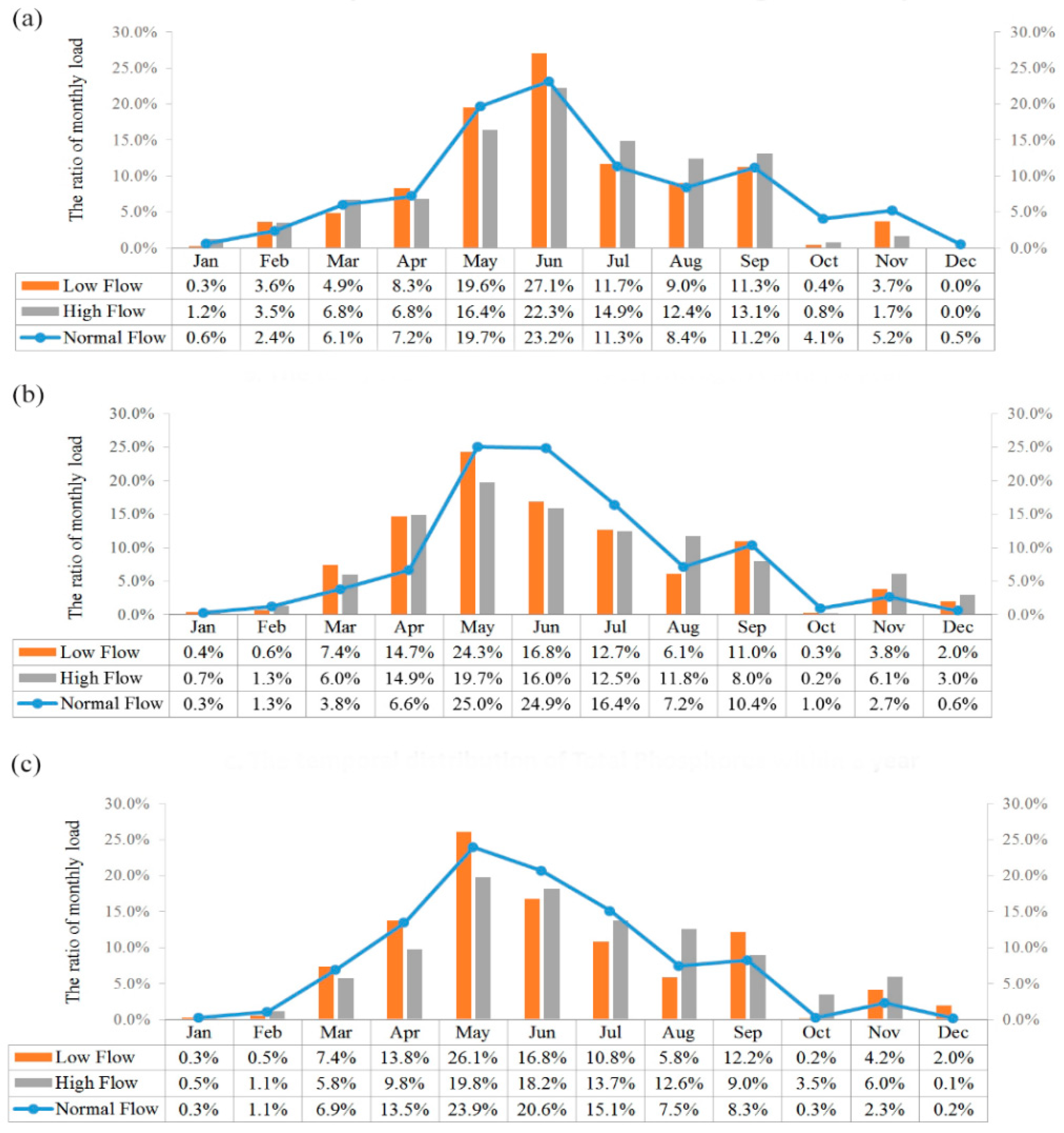
3.2.1. Temporal Distribution

Based on the simulation, we summarized the annual runoff and pollutants discharge. The temporal distribution of ammonia nitrogen (NH₄-N), total nitrogen (TN), and total phosphorus (TP) in different hydrological years is shown in Figure 5. From the figure, we can see that the pollution load from April to September (rainy season) accounted for a large proportion within a year, with the highest average in May and June. The contribution of NH₄-N, TN, and TP load during the flood season to the annual load is 81–87%, 82–90%, and 83–89%, with an average of 84%, 85%, and 86%, respectively. The change between different hydrological years was obvious, especially the variation in NPS temporal distribution over 12 months. For instance, the coefficient of variation in the high-flow year, 0.78–0.85 exactly, is lower than that in the low-flow year, 0.95–0.99 exactly. Correspondingly, the difference between the maximum and minimum value in the low-flow year is the largest.

The reason for this could be attributed to the relationship between precipitation and runoff, which is illustrated in Figure 6. It can be seen from Figure 6 that the runoff distribution shows a significant correlation with rainfall among the time series, and runoff also accumulates in months with abundant rainfall; the correlation coefficient (R) of runoff and rainfall over the year is 0.87. Since runoff generated from rainfall is a driver of NPS, the temporal distribution of NPS is affected by the central precipitation time. The average annual rainfall in the watershed is mainly concentrated in the period from April to September, accounting for about 80% of annual precipitation. Therefore, the temporal distribution of NPS also presents the same regularity. It approximately belongs to a normal distribution, and accumulates from April to September. This temporal distribution property of NPS is consistent with results from studies of similar watersheds [33], indicating the close relationship between the temporal distribution of NPS and local precipitation.

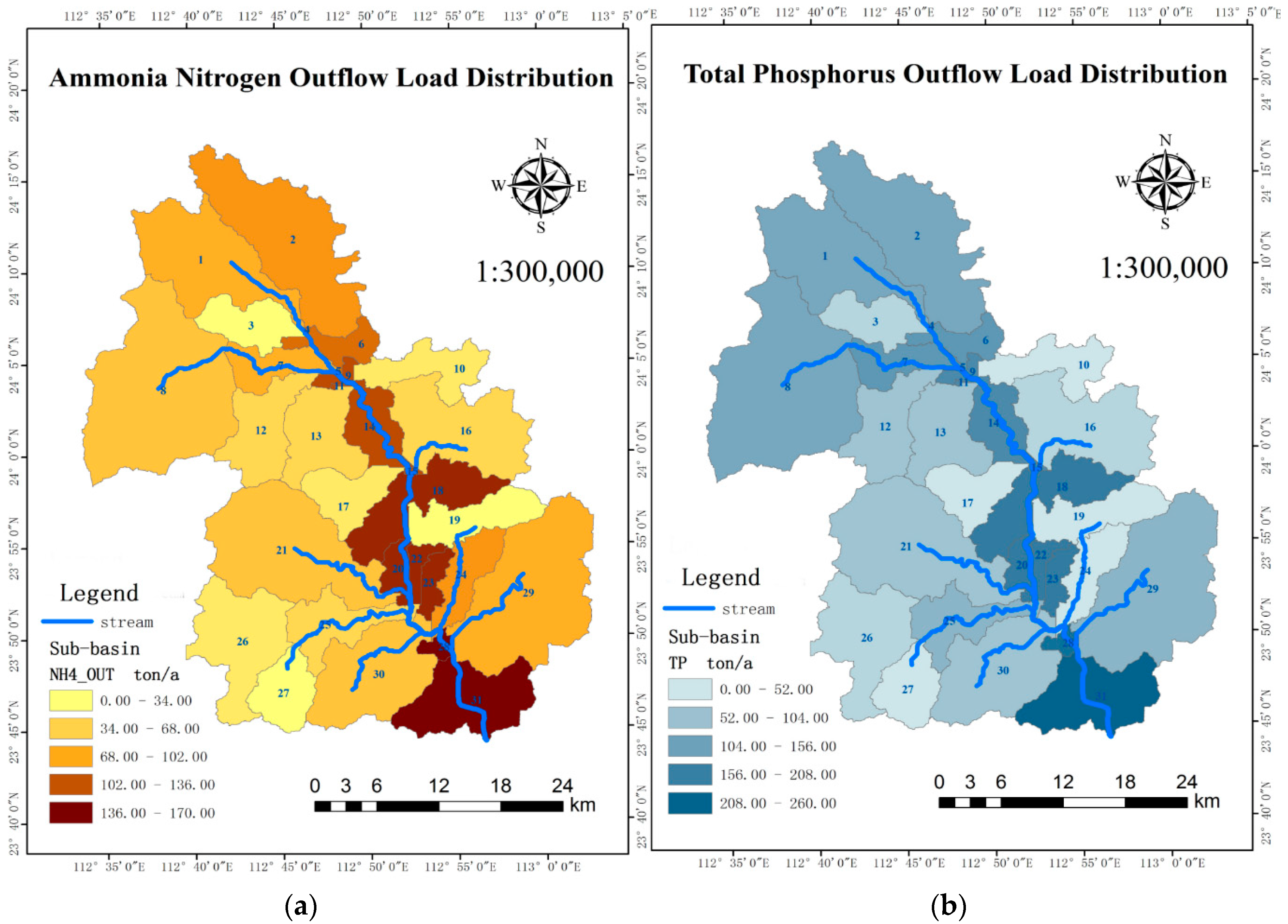
3.2.2. Spatial Distribution of NPS

The average annual load of NH₄-N and TP in the sub-basins is shown in Figure 7. Apparently, the area alongside the main stream has a high level of NPS load; for example, sub-basin Nos. 18, 20, and 31 have an average annual outflow load of around 160 tons of NH₄-N and 250 tons of TP. The northern part is at a medium level; the average annual outflow load is about 108 tons of NH₄-N and 165 tons of TP. The eastern area generates the least outflow load; for example, sub-basin Nos. 10 and 16 have an average annual load that is less than 30 tons of NH₄-N and 50 tons of TP. To conclude, the spatial distribution of NPS load is not evenly distributed, and mainly accumulates in the central and southern areas alongside the main stream.

As for the reason, since the stream is almost the lowest in topography, it is the destination at which surface runoff converges. Therefore, the NPS from upstream and remote sub-basins tends to converge in sub-basins alongside the stream, which has relatively low-altitude terrain. This is why the total load of NPS accumulates in the sub-basins alongside the main stream, especially in the southern area.

3.3. Analysis of the Generation Potential of NPS

The NPS load in sub-basin No. 31, for instance, does not generate itself, but accumulates from upstream sub-basins. Here, the question arises as to where the CSAs are; that is, which sub-basins generated a high level of NPS.

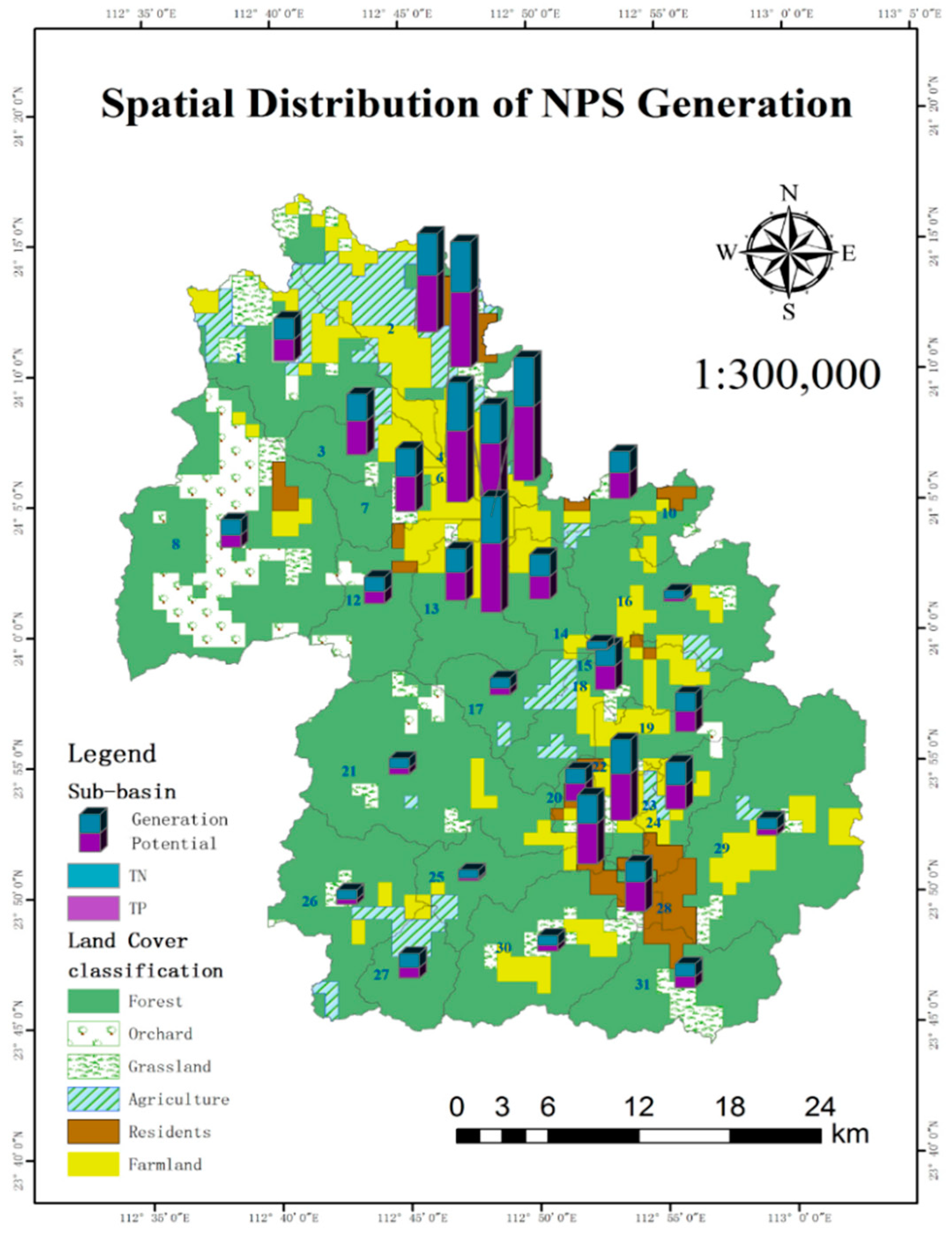
3.3.1. NPS Generation with Topography

Here, we analyze the generation distribution of NPS. It is focused on a sub-basin’s own pollution yield, and not the total outflow load that could be derived from other sub-basins. Researchers have usually focused on land cover with the spatial distribution of NPS, and studied the impact of land use change on NPS distribution [10,11,12]. Considering the gentle rolling/hilling topography and unchanged land cover of the watershed in the study area, we focused on NPS generation with topography. The main components of TN and TP generation under the topography conditions are depicted in Figure 8.

It can be seen that the spatial distribution of TN and TP generation shares some similarities. For example, the topography value and NPS generation have a negative correlation. In other words, the area where the terrain is low has a relatively high level of NPS yield. Another similarity is that, among the main components of TN and TP, the organic component, ORGN (Organic Nitrogen) and ORGP (Organic Phosphorus), is the dominant component. It is shown in Figure 8 that, regardless of whether the total height of the bar is high or not, the organic component occupies most of the total height: around 60–80%.

3.3.2. Accurate Positioning of NPS CSAs

In order to analyze the generation potential of NPS more thoroughly, the generation potential (Φ_i) of the 31 sub-basins was calculated and is shown in

Table 4. The value of the generation potential parameter Φ_i of all sub-basins for different pollutants.

SUB No.	AREA km2	ORGN	NH4	NSURQ	TN	ORGP	SOLP	SEDP	TP	TN + TP
4	0.333	4.298	2.010	1.646	3.321	4.219	0.231	4.027	3.706	7.028
5	0.405	4.227	0.756	1.618	3.235	4.150	0.227	4.002	3.654	6.890
9	6.598	4.103	2.053	1.429	3.169	4.027	0.265	3.791	3.532	6.700
11	0.586	3.902	1.933	1.533	3.016	3.829	0.410	3.990	3.459	6.475
2	140.010	3.041	2.150	1.814	2.519	3.097	1.454	3.572	3.004	5.523
6	22.206	3.013	2.067	1.696	2.476	2.960	0.713	2.790	2.658	5.134
23	13.611	2.634	2.408	1.243	2.178	2.584	0.498	2.658	2.353	4.532
22	11.359	2.330	2.503	0.869	1.863	2.295	0.181	2.184	2.022	3.885
7	31.789	2.017	0.767	1.297	1.716	1.990	0.957	1.772	1.821	3.537
3	37.105	1.946	0.039	1.247	1.630	1.919	0.833	1.746	1.754	3.384
13	56.975	1.622	0.467	1.128	1.422	1.596	0.812	1.476	1.478	2.900
28	6.957	1.705	2.529	0.486	1.340	1.695	0.098	1.450	1.454	2.794
10	41.917	1.451	0.157	0.956	1.267	1.427	0.689	1.553	1.366	2.633
24	36.875	1.365	3.213	0.868	1.370	1.340	0.588	1.377	1.259	2.629
18	64.044	1.339	2.642	0.977	1.281	1.315	0.715	1.370	1.256	2.537
14	36.256	1.299	2.460	1.182	1.274	1.278	0.912	1.209	1.220	2.494
1	105.800	1.132	1.770	1.196	1.124	1.190	1.576	1.409	1.282	2.406
19	45.810	1.150	0.092	0.881	1.079	1.130	0.713	1.118	1.078	2.157
20	12.944	0.990	2.789	0.512	0.919	0.984	0.346	0.832	0.876	1.795
8	204.890	0.712	0.297	1.166	0.802	0.707	1.314	0.564	0.748	1.551
12	56.125	0.689	0.534	1.030	0.778	0.683	1.087	0.545	0.701	1.479
27	37.361	0.559	0.046	1.005	0.711	0.591	1.183	0.568	0.656	1.367
31	73.509	0.634	2.555	0.668	0.711	0.629	0.750	0.576	0.632	1.344
17	38.651	0.418	0.196	0.721	0.537	0.414	0.853	0.326	0.447	0.984
29	158.660	0.329	0.958	0.888	0.543	0.327	1.092	0.292	0.410	0.953
21	144.490	0.366	0.386	0.682	0.502	0.362	0.844	0.303	0.406	0.908
30	94.306	0.319	0.521	0.726	0.493	0.316	0.898	0.276	0.377	0.870
26	84.099	0.284	0.128	0.723	0.462	0.280	0.879	0.244	0.343	0.806
16	96.152	0.161	0.343	0.614	0.381	0.159	0.803	0.148	0.233	0.614
25	45.592	0.139	0.225	0.681	0.366	0.138	0.892	0.134	0.226	0.592
15	1.134	0.063	2.430	0.382	0.362	0.062	0.521	0.054	0.114	0.477

. In the table, Φ_i > 1 indicates that the generation potential of this sub-basin is higher than average; considering the multiple influences of nitrogen and phosphorus, the value of Φ_i > 2 in the “TN + TP” column means the same. We arranged the 31 sub-basins based on a descending contribution to NPS generation; high generators are highlighted in gray.

Table 4 shows that the sub-basins with a high level of generation potential are Nos. 2–7, 9, 11, 22, and 23, for which the value of Φ_i is over 3.0, which means that the NPS generation potential is over 1.5 times the average level. To answer the question of where the CSAs are, a large proportion is from the northeast sub-basins with lower terrain that is mainly used for agricultural applications, accounting for 53% of the total NPS generation of the watershed. The value of Φ₃₁ in the “TN + TP” column is less than 2.0; therefore, the generation potential at sub-basin No. 31 is less than the average level.

Additionally, we classified the sub-basins into three ranks (relatively low, medium, relatively high) based on Φ_i, the generation potential of “TN + TP”. In the first rank, Φ_i is less than 1.6. This rank generates little pollution; examples are sub-basin Nos. 15, 17, and 26. The terrain is relatively high, and the land cover is mainly thick evergreen forest. Although precipitation is relatively high, the densely distributed vegetation alleviates pollution loss by rainfall. In the second rank, Φ_i is between 1.6 and 3.0. This rank generates a medium level of NPS; examples are sub-basin Nos. 18, 19, and 20. The terrain is relatively low. The land cover contains forest, grassland, and small amount of agriculture. There is a medium amount of precipitation. In the third rank, Φ_i is greater than 3.0. This rank generates a relatively high level of pollution; examples are sub-basin Nos. 2, 6, and 9. The terrain is low and the precipitation is relatively high. The land cover is mainly farmland and residential. Without densely distributed forest, the last rank generates a large amount of NPS pollution by human activities and rainfall scouring. This is consistent with the results of studies on the impact of land cover change on NPS pollution [12] that show that an increase in farmland or residential areas and a reduction in green vegetation would increase the NPS pollution to a large extent [10,11,12,13,14]. These are the CSAs that demand special attention. The generation potential of “TN + TP” and land cover is depicted in Figure 9.

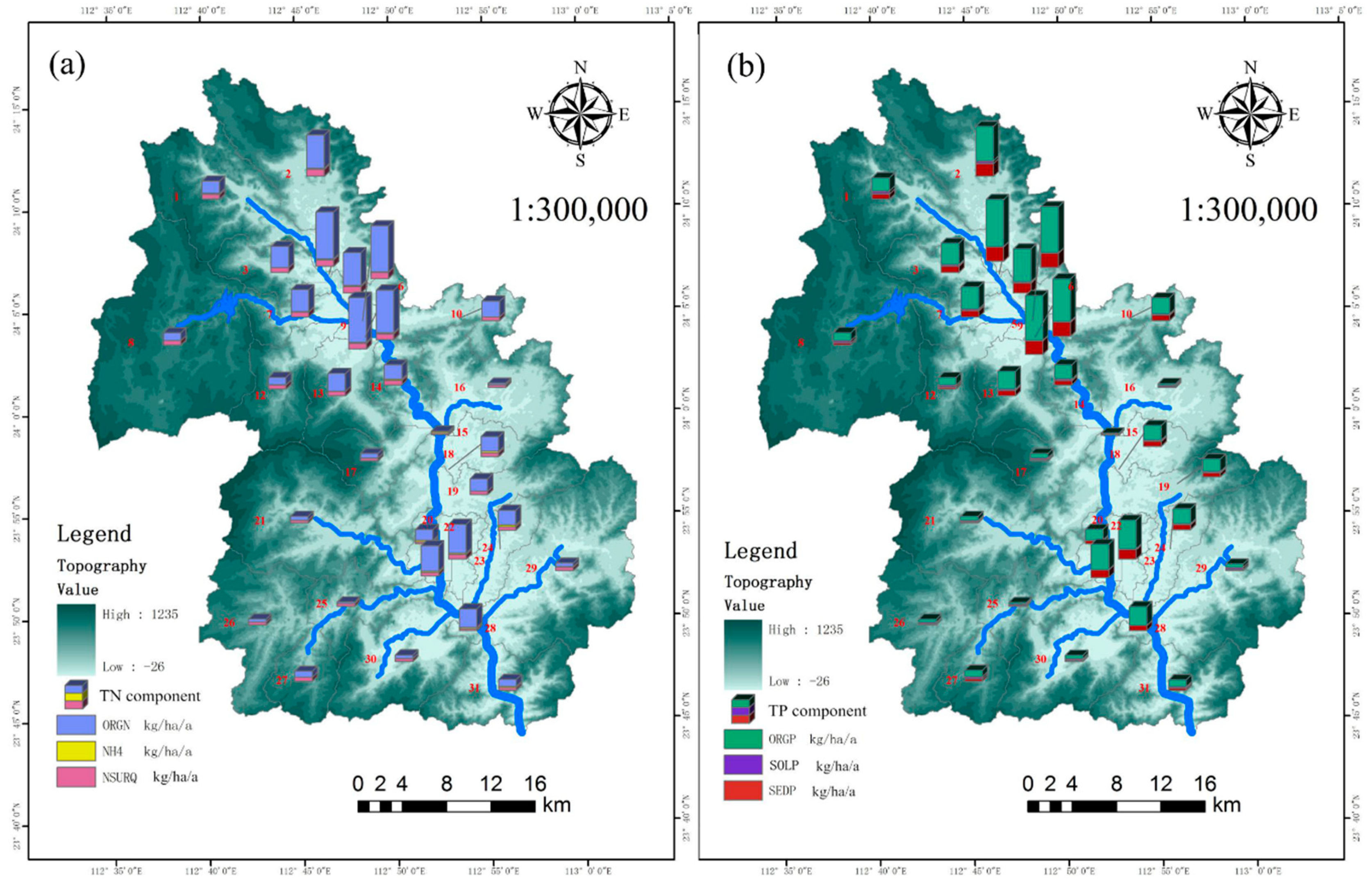
3.3.3. The Main NPS Pollutants in Sub-Basins

Compared with the load per hectare, which is applied widely in NPS studies [4,5,6], the introduction of the NPS generation potential parameter Φ_i has several advantages. For a certain NPS pollutant or a combination of several pollutants, the generation potential parameter Φ_i can tell us which are the high generators (CSAs) and the severity of their pollution. As for load per hectare, for instance, researchers have set 5 kg/ha TN as the standard of NPS CSAs when studying the head stream watershed of the Yellow River in China [34]. However, this standard could not be applied to other watersheds or other pollutants under different pollution conditions. Nevertheless, the introduction of the dimensionless parameter Φ_i can help us to make progress. The value of Φ_i > 3 in “TN + TP” or Φ_i > 1.5 in other pollutants designates the high NPS generators or CSAs, regardless of the background or condition of the watershed. Moreover, for a certain district, the comparison of Φ_i of different pollutants can provide information on the main local pollutants. For instance, in Table 4, for sub-basin No. 18, Φ_ORGN = 1.339, Φ_NH4 = 2.642, and Φ_NSURQ = 0.977, which means that the organic nitrogen and NO₃ in the surface runoff are average, while the ammonia nitrogen is over 2 times the average level. Thus, in sub-basin No. 18, the main pollutant is ammonia nitrogen, which demands that focus be placed on relevant control measures. In summary, the sub-basins for which the main pollutant is ammonia nitrogen are Nos. 1, 13, 14, 18, 20, 22–24, 28, and 31, which are located in the central and southern districts alongside the main stream, and account for 26.67% of the whole watershed. The sub-basins for which the main pollutants are sediment and organic nitrogen are Nos. 2–7, 9, and 10, which are mainly located in the northern districts for farming or agricultural usage, and account for 16.43% of the total area of the watershed. The sub-basins for which the main pollutant is biological oxygen demand (BOD) are Nos. 12, 13, 16, 17, 19, 21, and 25–27, which are mainly located in low-NPS-generation areas with natural vegetation, and account for 35.47% of the total area of the Binjiang watershed.

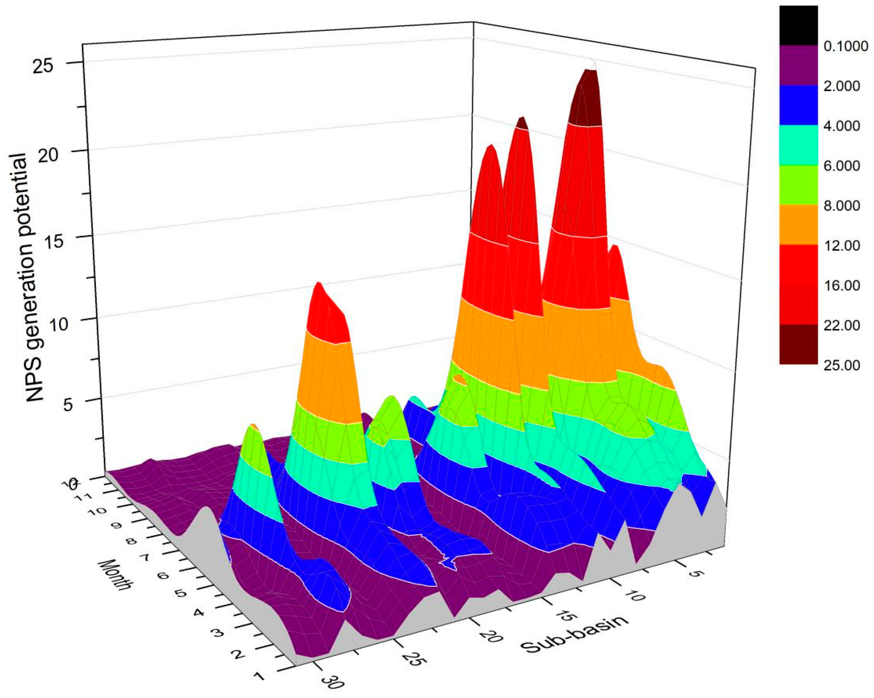
3.3.4. Temporal Distribution of NPS CSAs

We also analyzed the generation potential of a combination of TN and TP in each sub-basin during a 12-month period, as depicted in Figure 10. As for high generators, the temporal distribution of NPS tends to accumulate from April to July, accounting for 69% of the annual yield, which will assist the temporal NPS control in certain areas.

As shown in the figure, the x-axis represents the 31 sub-basins, the y-axis represents the 12 months in a year, and the z-axis represents the generation potential of NPS. It can be seen that the distribution of NPS generation potential in the study area is not balanced, whether on the time scale or the spatial scale. Firstly, the x-axis of the geographical space is from right to left. It can be seen that the upstream area (sub-basin Nos. 1–11) has a relatively high potential for NPS generation, followed by the middle districts (sub-basin Nos. 22 and 23). As for the central margin and southern part of the watershed, only sub-basin No. 28 has a slightly higher NPS generation potential; the overall NPS generation potential throughout the 12-month period is relatively low. Moreover, from January to December, it can be seen that the highest NPS generation occurs in May and June, and is concentrated mainly from April to July. In addition, for some CSAs (sub-basin Nos. 2–6 and 9), the NPS generation potential in February and March is also relatively high. Researchers studying the NPS in farmland in southern China obtained similar results, except for the rainy season. February and March also have high NPS load [33], which could be attributed to the tillage and fertilization of farmland in this period. Therefore, during this time, we should focus on these particular areas, especially those used for farming.

3.4. NPS Control Management

3.4.1. Scenario

In this study, a riparian filter strip was set for the hydrological response unit around the main stream and tributary of the Binjiang river, mainly in the NPS CSAs (sub-basin Nos. 1–11). The river bank’s average slope ratio is 1:8. The vegetation is shrub herb in natural grassland. The filter strip’s width was designed to be 3–30 m. The riparian buffer strips were added to the management module of SWAT, and their reduction effects on different NPS pollutants were simulated.

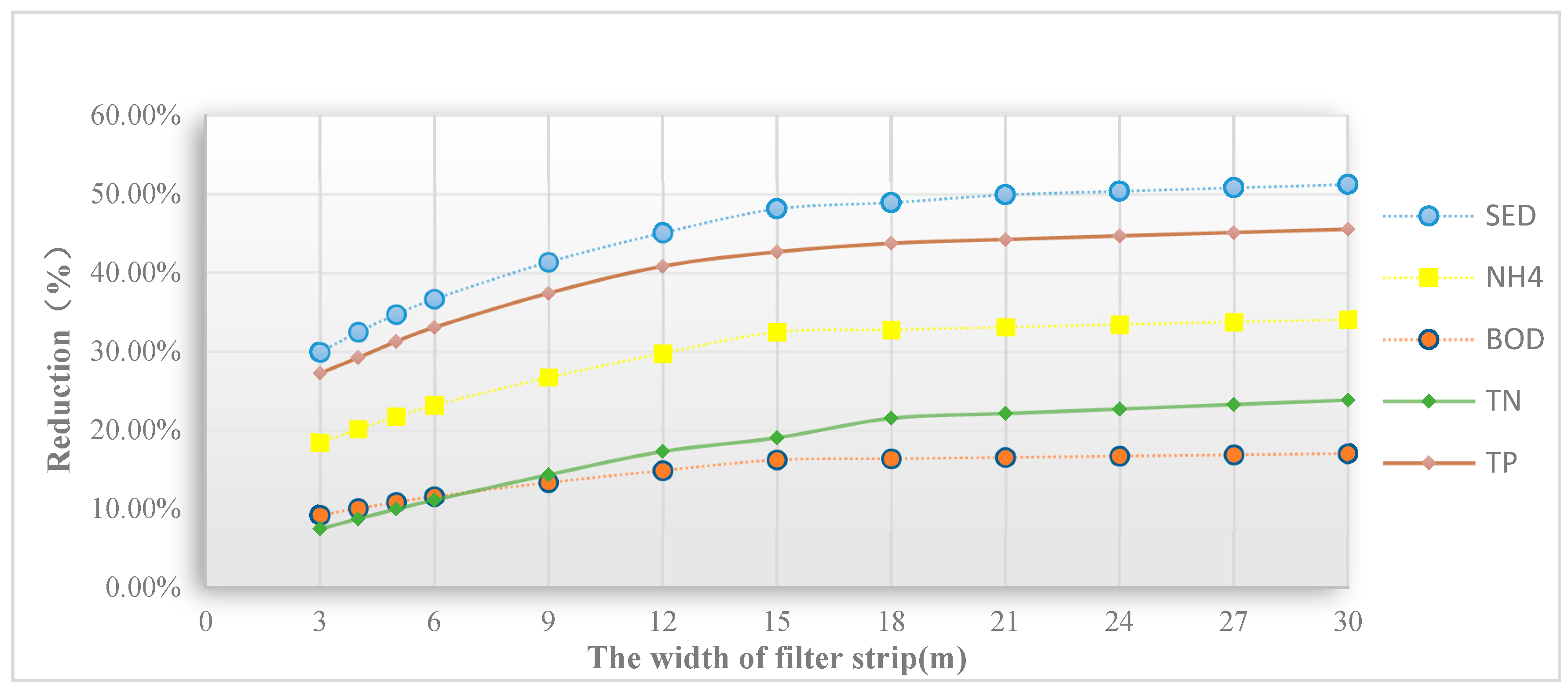
3.4.2. Simulation and Best Selection

Based on the above scenario, the improved SWAT model was used to simulate the generation of NPS pollutants with different filter strips. The evaluated pollutants were SED (sediment or suspended particulate), BOD (biochemical oxygen demand), NH₄ (ammonia nitrogen), TN (total nitrogen), and TP (total phosphorus). With the original condition as a blank scenario, we simulated the reduction effects of the riparian filter strips on various pollutants with different structural designs, depicted in Figure 11. The NPS generation and reduction rate are listed in

Table 5. The NPS outflow load and reduction in different filter strip scenarios.

Width of Filter Strip (m)	Load/Reduction	SED	NH4	BOD	TN	TP
	Original Load (kg/ha)	65.882	2.318	25.741	69.330	6.653
3	load (kg/ha)	51.663	2.016	24.069	65.819	5.344
	Reduction (%)	21.58%	13.00%	6.50%	5.06%	19.67%
4	load (kg/ha)	48.417	1.943	23.662	65.022	5.046
	Reduction (%)	26.51%	16.16%	8.08%	6.21%	24.15%
5	load (kg/ha)	46.185	1.891	23.371	64.167	4.840
	Reduction (%)	29.90%	18.42%	9.21%	7.45%	27.24%
6	load (kg/ha)	44.482	1.851	23.150	63.269	4.710
	Reduction (%)	32.48%	20.13%	10.07%	8.74%	29.21%
8	load (kg/ha)	43.007	1.814	22.944	62.417	4.572
	Reduction (%)	34.72%	21.73%	10.87%	9.97%	31.27%
9	load (kg/ha)	41.729	1.781	22.760	61.615	4.453
	Reduction (%)	36.66%	23.16%	11.58%	11.13%	33.07%
10	load (kg/ha)	38.629	1.699	22.304	59.391	4.163
	Reduction (%)	41.37%	26.71%	13.35%	14.34%	37.42%
12	load (kg/ha)	36.193	1.628	21.911	57.333	3.936
	Reduction (%)	45.06%	29.76%	14.88%	17.30%	40.84%
15	load (kg/ha)	34.181	1.565	21.563	54.744	3.815
	Reduction (%)	48.12%	32.47%	16.23%	19.04%	42.66%
18	load (kg/ha)	33.659	1.559	21.526	54.416	3.742
	Reduction (%)	48.91%	32.75%	16.37%	21.51%	43.75%
21	load (kg/ha)	33.007	1.551	21.481	54.001	3.710
	Reduction (%)	49.90%	33.10%	16.55%	22.11%	44.24%
24	load (kg/ha)	32.704	1.543	21.438	53.595	3.679
	Reduction (%)	50.36%	33.43%	16.72%	22.70%	44.69%
27	load (kg/ha)	32.415	1.535	21.397	53.197	3.651
	Reduction (%)	50.80%	33.75%	16.88%	23.27%	45.13%
30	load (kg/ha)	32.138	1.528	21.358	52.808	3.623
	Reduction (%)	51.22%	34.06%	17.03%	23.83%	45.54%

.

As shown above, from the perspective of pollutants, the filter strip has the best control effect on SED; the average annual reduction rate reaches 41–50%. The reduction rate of the average annual output of TP reaches 37–45%. Researchers have studied the effectiveness of grass strips on water quality, and the results showed that the effects of grass strips on the removal of sediments and nutrients were significant: over 20% in sediments and TP [35,36]. However, the reduction effect on ammonia nitrogen and TN is relatively low. The average annual reduction rate of TN, for instance, is only 10–22%. Similarly, the implementation of a 25% grass strip in Central Indiana, United States, led to a reduction in nitrogen and BOD loads between 2.41% and 5.75% [37]. The reason for this is that inorganic nitrogen migrates with surface runoff in a dissolved state. Organic and mineral phosphorus migrate and adhere to sediment in surface runoff. According to the literature, more than 70% of phosphorus and about 20% of nitrogen (mainly organic nitrogen) accumulate in this way in catchment area [38]. Since filter strips have a better sedimentation effect on SED, the TP adsorbed to particulate matter is also removed. Ammonia nitrogen, nitrate nitrogen, and BOD are mainly removed by absorption of plant roots and the degradation of microorganisms. Because of the slope of the river bank, the hydraulic retention time of pollution flowing through a riparian filter strip is insufficient for absorption and degradation; therefore, the reduction effect of TN and BOD is lower. Similarly, Stagge [39] demonstrated the performance of grass swales with experimental methods to measure pollutant concentrations in inflow and outflow, and found that grass swales reduced sediment and TP by 40–85% and 20–45%, respectively, while the reduction in TN and BOD was less than 15%.

From the perspective of structure design, there is a certain nonlinear relationship between the design scenarios and the efficiency of the reduction in the pollutants. As shown in the figure, when the width of the buffer strip is less than 15 meters, the reduction effect of NPS pollutants gradually increases; that is, there is a significant positive correlation. When the width of the filter strip is greater than 15 meters, the control effect on NPS pollutants tends towards stability. Taking NH₄ and TP as examples, the relationship between average reduction rate (y) and riparian buffer strip width (x) is similar to a logarithmic equation. Based on the data from Table 5, SPSS software was used to solve the fitting regression equation y = a∙ln(x) + b. The solved nonlinear fitting regression equation is as follows:

y_NH4 = 0.0694ln(x) + 0.1157

(8)

y_TP = 0.0827ln(x) + 0.1876.

(9)

The fitting degree of this equation is fairly high. The relative error (Re) of NH₄ is only 6.81%, and the determination coefficient (R²) of NH₄ is 0.9804. The relative error (Re) of TP is only 4.16%, and the R² of TP is as high as 0.9882. For areas with similar natural conditions (a subtropical monsoon climate, clay-loam soil, and non-urban areas), the fitting equation can be used to estimate the NPS reduction effect of riparian filter strips in the absence of numerical data for simulation. Researchers have studied the width of a filter strip and its pollution reduction effect in large flat watersheds. The results showned that the 15 m filter strip is slightly better than the 10 m filter strip, which is apparently better than the 5 m filter strip. In general, a filter strip that is 10–15 m in width can intercept 3–45% of TN, and 30–80% of TP [36,37,38,39,40]. Similarly, considering the reduction effect and cost, a 15 m filter strip alongside the main stream is suggested, as it can produce a reduction effect on sediment (SED), total nitrogen (TN), and total phosphorus (TP) of up to 48.12%, 19.04%, and 42.33%, respectively.

4. Conclusions

Because of the limitations to the surface runoff module in SWAT, in order to avoid deviation in simulations caused by a single initial abstraction value, this paper adopted the method of a segmentation value of initial abstraction to improve the model, named SWAT-m. By data collection, we established databases for topography, soil, land use, and weather. Then, we performed runoff and NPS pollutant simulations. The results enabled us to draw the following conclusions:

Through the comparison of runoff simulations using SWAT and SWAT-m, we obtained that the modified model has better simulation accuracy. In particular, during the validation period, the evaluation indicators are: Ens = 0.72, R² = 0.75, and Re = 27% (SWAT); Ens = 0.89, R² = 0.91, and Re = 14% (SWAT-m). The modified model improves the simulation accuracy by 23.61% (Ens) and 21.33% (R²), indicating its better adaptability to simulate extensive watershed pollution under various natural conditions.

As for NPS pollutants, simulation by SWAT-m also complies with the standard for accuracy. Thus, it was applied in further research. For a watershed in a subtropical monsoon climate, the temporal distribution of NPS approximately belongs to a normal distribution, and accumulates from April to September. The contribution of TN and TP in the rainy season to the annual load is 82–90% and 83–89%, with an average of 85% and 86%, respectively. Additionally, the average annual NPS load is not evenly distributed, and mainly accumulates in the central and southern areas alongside the main stream.

As for the spatial distribution of NPS, the topography value and NPS generation have a negative correlation. Through the generation potential parameter Φ_i, we obtained the descending order of all sub-basins in terms of their contribution to total NPS generation. The CSAs were found to be mostly northeast sub-basins with lower terrain that is used mainly for agricultural applications, accounting for about 53% of the total generation. The temporal distribution of high NPS generators accumulated from April to July, reaching 69% of the annual load. Also, through a comparison of Φ_i between pollutants, we found that the main pollutants of CSAs are organic nitrogen (ORGN), ammonia nitrogen (NH4), and particulate matter (SED); the main pollutant for the central and southern areas alongside the main stream is ammonia nitrogen.

By simulating the impact of a riparian filter strip on NPS pollution in CSAs, it was shown that filter strips efficiently reduce particulate matter (SED) and total phosphorus (TP) by up to 48.12% and 42.33%, respectively. The reduction effect on pollutants and the designed width of the filter strip indicated an approximate logarithmic relationship, which could be applied to similar watersheds without numerical data for simulation. When the buffer width reaches 15 meters, the reduction rate tends towards stability; thus, the recommended design is a 15-m wide filter strip, with a slope ratio of 1:8, that is covered with local natural herbaceous vegetation alongside the river.

Because of limitations in time, researchers, and measured data, we only validated two kinds of pollutants (ammonia nitrogen and total phosphorus). Further research may simulate the other main components of NPS, such as BOD (biochemical oxygen demand).

As a result of the research in this study, we can accurately position the high generators of NPS pollution and its accumulation time. Further research could focus on control measures other than filter strips to decrease NPS. The results of this study are of practical significance to the management of NPS pollution in watersheds under similar conditions.

References

1. Lee, S.I. Nonpoint source pollution. Fisheries 1979, 2, 50–52. [Google Scholar]
2. Di, L.M.; Arnold, J.G. Formulation of a hybrid calibration approach for a physically based distributed model with NEXRAD data input. J. Hydrol. 2004, 298, 136–154. [Google Scholar]
3. Deslandes, J.; Michaud, A.; Bonn, F. Use of GIS and remote sensing to develop indicators of phosphorus non-point source pollution in the Pike River basin. In Lake Champlain: Partnerships and Research in the New Millennium; Springer US: New York NY, USA, 2004; pp. 271–290. [Google Scholar]
4. Sumant, D.; Surinder, K.; Nilanchal, P. Hydrological modeling in middle Narmada Basin, India using SWAT model; Lap Lambert Academic Publishing: Saarbrücken, Germany, 2015. [Google Scholar]
5. Hu, X.; McIsaac, G.F.; David, M.B.; Louwers, C.A.L. Modeling riverine nitrate export from an east-central Illinois watershed using SWAT. J. Environ. Qual. 2007, 36, 996–1005. [Google Scholar] [CrossRef]
6. Akhavan, S.; Abedi-Koupai, J.; Mousavi, S.F.; Afyuni, M.; Eslamian, S.S. Application of SWAT model to investigate nitrate leaching in Hamadan–Bahar Watershed, Iran. Agric. Ecosyst. Environ. 2010, 139, 675–688. [Google Scholar] [CrossRef]
7. Santhi, C.; Srinivasan, R.; Arnold, J.; Williams, J. A modeling approach to evaluate the impacts of water quality management plans implemented in a watershed in Texas. Environ. Model. Softw. 2006, 21, 1141–1157. [Google Scholar] [CrossRef]
8. Song, L.X.; Liu, P. Study on Agricultural Non-point Source Pollution Based on SWAT. Environ. Mater. Environ. Manag. 2010, 113–116, 390–394. [Google Scholar] [CrossRef]
9. Choi, W. Catchment-scale hydrological response to climate-landuse combined scenarios: A case study for the Kishwaukee River Basin, Illinois. Phys. Geogr. 2008, 29, 79–99. [Google Scholar] [CrossRef]
10. Du, J.; Qian, L.; Rui, H.; Zuo, T.; Zheng, D.; Xu, Y.; Xu, C.Y. Assessing the effects of urbanization on annual runoff and flood events using an integrated hydrological modeling system for Qinhuai River basin, China. J. Hydrol. 2012, 4, 127–139. [Google Scholar] [CrossRef]
11. Wilson, C.O.; Weng, Q. Simulating the impacts of future land use and climate changes on surface water quality in the Des Plaines River watershed, Chicago Metropolitan Statistical Area, Illinois. Sci. Total Environ. 2011, 409, 4387–4405. [Google Scholar] [CrossRef]
12. Chung, E.; Park, K.; Lee, K.S. The relative impacts of climate change and urbanization on the hydrologic response of a Korean urban watershed. Hydrol. Process. 2011, 25, 544–560. [Google Scholar] [CrossRef]
13. Cuo, L.; Lettenmaier, D.P.; Alberti, M.; Richey, J.E. Effects of a century of land cover and climate change on the hydrology of the Puget Sound basin. Hydrol. Process. 2009, 23, 907–933. [Google Scholar] [CrossRef]
14. Zhang, P.; Liu, Y.H.; Pan, Y.; Yu, Z.R. Land use pattern optimization based on CLUE-S and SWAT models for agricultural non-point source pollution control. Math. Comput. Model. 2013, 58, 588–595. [Google Scholar] [CrossRef]
15. Mishra, S.K.; Singh, V.P. Validity and extension of the SCS-CN method for computing infiltration and rainfall-excess rates. Hydrol. Process. 2004, 18, 3323–3345. [Google Scholar] [CrossRef]
16. Nagarajan, N.; Poongothai, S. Spatial Mapping of Runoff from a Watershed Using SCS-CN Method with Remote Sensing and GIS. J. Hydrol. Eng. 2012, 17, 1268–1277. [Google Scholar] [CrossRef]
17. Arnold, J.G.; Kiniry, J.R.; Srinivasan, R.; Williams, J.R.; Haney, E.B.; Neitsch, S.L. Soil and Water Assessment Tool Input/Output File Documentation Version 2009; Texas Water Resources Institute Technical Report No. 365[R]; Texas A&M University System College Station: College Station, TX, USA, 2011. [Google Scholar]
18. Neitsch, S.L.; Arnold, J.G.; Kiniry, J.R.; Williams, J.R. Soil and Water Assessment Tool Theoretical Documentation (Mannual); Blackland Research Center, Texas Agricultural Experiment Station and Grassland, Soil and Water Research Laboratory: Temple, TX, USA, 2005. [Google Scholar]
19. Brown, L.C.; Barnwell, T.O. The Enhanced Stream Water Quality Models QUAL2E and QUAL2E-UNCAS: Documentation and User Model; USEPA: Athens, GA, USA, 1987. [Google Scholar]
20. Mishra, S.K.; Sahu, R.K.; Eldho, T.I. An improved I-a-S relation incorporating antecedent moisture in SCS-CN methodology. Water Resour. Manag. 2006, 20, 643–660. [Google Scholar] [CrossRef]
21. Woodward, D.E.; Hawkins, R.H. Runoff Curve Number Method: Examination of the Initial Abstraction Ratio; World Water and Environmental Resources Congress: Pennsylvania, PA, USA, 2003. [Google Scholar]
22. International Scientific Data Service Platform. Available online: http://datamirror.csdb.cn/index.jsp (accessed on 10 May 2019).
23. National Earth System Science Data Sharing Infrastructure Website. Available online: http://www.geodata.cn/ (accessed on 10 May 2019).
24. Guangdong Soil Survey Office. Guangdong Soil; Beijing Science Press: Beijing, China, 1993. [Google Scholar]
25. Soil Science, Chinese Academy of Science Website. Available online: http://www.soil.csdb.cn/ (accessed on 10 May 2019).
26. China Meteorological Science Data Sharing Service Network. Available online: https://data.cma.cn/data/detail/ (accessed on 10 May 2019).
27. Basnyat, P.; Teeter, L.D.; Lockaby, B.G.; Flynn, K.M. The use of remote sensing and GIS in watershed level analyses of non-point source pollution problems. For. Ecol. Manag. 2000, 128, 65–73. [Google Scholar] [CrossRef]
28. Cibin, R.; Chaubey, I.; Engel, B. Simulated watershed scale impacts of corn stover removal for biofuel on hydrology and water quality. Hydrol. Process. 2012, 26, 1629–1641. [Google Scholar] [CrossRef]
29. Moriasi, D.; Arnold, J.; Van, L.M.; Bingner, R.; Harmel, R.; Veith, T. Model evaluation guidelines for systematic quantification of accuracy in watershed simulations. Trans. ASABE 2007, 50, 885–900. [Google Scholar] [CrossRef]
30. Neitsch, S.L.; Arnold, J.G.; Kiniry, J.R.; Williams, J.R.; King, K.W. Soil and Water Assessment Tool Theoretical Documentation Version 2000; Texas Water Resources Institute: College Station, TX, USA, 2002. [Google Scholar]
31. Abbaspour, K.C.; Vejdani, M.; Haghighat, S. SWAT-CUP Calibration and Uncertainty Programs for SWAT. In Proceedings of the International Congress on Modelling & Simulation Land Water & Environmental Management Integrated Systems for Sustainability, Christchurch, New Zealand, 10–13 December 2007. [Google Scholar]
32. Hao, F.H.; Cheng, H.G.; Yang, S.T. Non-Point Source Pollution Model: Theoretical Method and Application; Chinese Environmental Science Press: Beijing, China, 2006. [Google Scholar]
33. Jiang, J.; Li, S.; Hu, J. A modeling approach to evaluating the impacts of policy-induced land management practices on non-point source pollution: A case study of the Liuxi River watershed, China. Agric. Water Manag. 2014, 131, 1–16. [Google Scholar] [CrossRef]
34. Ouyang, W.; Wang, X.L.; Hao, F.H.; Srinivasan, R. Temporal-spatial dynamics of vegetation variation on non-point source nutrient pollution. Ecol. Model. 2009, 220, 2702–2713. [Google Scholar] [CrossRef]
35. Lee, M.; Park, G.; Park, M.; Park, J.; Lee, J.; Kim, S. Evaluation of non-point source pollution reduction by applying Best Management Practices using a SWAT model and QuickBird high resolution satellite imagery. J. Environ. Sci. 2010, 22, 826–833. [Google Scholar] [CrossRef]
36. Dennis, L.C.; Peter, J.V.; Keith, I. Modeling non-point source pollution in vadose zone with GIS. Environ. Sci. Technol. 1997, 8, 2157–2175. [Google Scholar]
37. Liu, Y.; Bralts, F.V.; Engel, A.B. Evaluating the effectiveness of management practices on hydrology and water quality at watershed scale with a rainfall-runoff model. Sci. Total Environ. 2015, 511, 298–308. [Google Scholar] [CrossRef]
38. Schaffner, M.; Bader, H.P.; Scheidegger, R. Modeling the contribution of point sources and non-point sources to Thachin River water pollution. Sci. Total Environ. 2009, 407, 4902–4915. [Google Scholar] [CrossRef]
39. Stagge, J.H.; Davis, A.P.; Jamil, E.; Kim, H. Performance of grass swales for improving water quality from highway runoff. Water Res. 2012, 46, 6731–6742. [Google Scholar] [CrossRef]
40. Gorsevski, P.V.; Boll, J.; Gomezdelcampo, E.; Brooks, E.S. Dynamic riparian buffer widths from potential non-point source pollution areas in forested watersheds. For. Ecol. Manag. 2008, 256, 664–673. [Google Scholar] [CrossRef]
Figure 1. The location of the research area. The upper half is the location of China, the lower half shows the contours of Guangdong Province, and yellow area in the middle depicts the research area.
Water 11 00993 g001
Figure 2. The soil classification of the study area. Streams are depicted by blue lines.
Water 11 00993 g002
Figure 3. The division of the study area into sub-basins and the hydrologic stations in the study area. The topography is described by the gradient color of grass green. Streams are shown by blue lines. Hydrologic stations are denoted by yellow points. Weather stations are depicted by orange pentagons. Sub-basins are numbered in dark blue.
Water 11 00993 g003
Figure 4. The calibration and validation of (a) runoff, (b) ammonia nitrogen, and (c) total phosphorus. Black points indicate observed values. Blue lines indicate simulated values.
Water 11 00993 g004
Figure 5. The percentage of monthly load of (a) ammonia nitrogen, (b) total nitrogen, and (c) total phosphorus in different hydrological years.
Water 11 00993 g005
Figure 6. The correlation between precipitation and runoff during the simulation period.
Water 11 00993 g006
Figure 7. The spatial distribution of the average annual load of ammonia nitrogen (a) and total phosphorus (b). Sub-basins are numbered in dark blue with gray boundary lines.
Water 11 00993 g007
Figure 8. The spatial distribution of Total Nitrogen (TN) (a) and Total Phosphorus (TP) (b) generation. The bars indicate the average yield of TN or TP per unit area. In the left panel, blue bars denote Organic Nitrogen (ORGN), yellow denotes Ammonia Nitrogen (NH4), and rose red denotes NO3 in surface runoff (NSURQ). In the right panel, green denotes Organic Phosphorus (ORGP), purple denotes Soluble Phosphorus (SOLP), and red denotes Mineral Phosphorus (SEDP). Sub-basins are numbered in red color with gray boundary lines.
Water 11 00993 g008
Figure 9. The spatial distribution of non-point source pollution (NPS) generation potential. The bars stand for the NPS generation potential parameter Φi of each sub-basin. Blue denotes TN, and purple denotes TP.
Water 11 00993 g009
Figure 10. The generation potential of “TN + TP” in the sub-basins during a 12-month period.
Water 11 00993 g010
Figure 11. The design of the riparian filter strip and its impact on pollution reduction.
Water 11 00993 g011