Coupling between Hydrodynamics and Chlorophyll a and Bacteria in a Temperate Estuary: A Box Model Approach


Abstract
1. Introduction
2. Materials and Methods
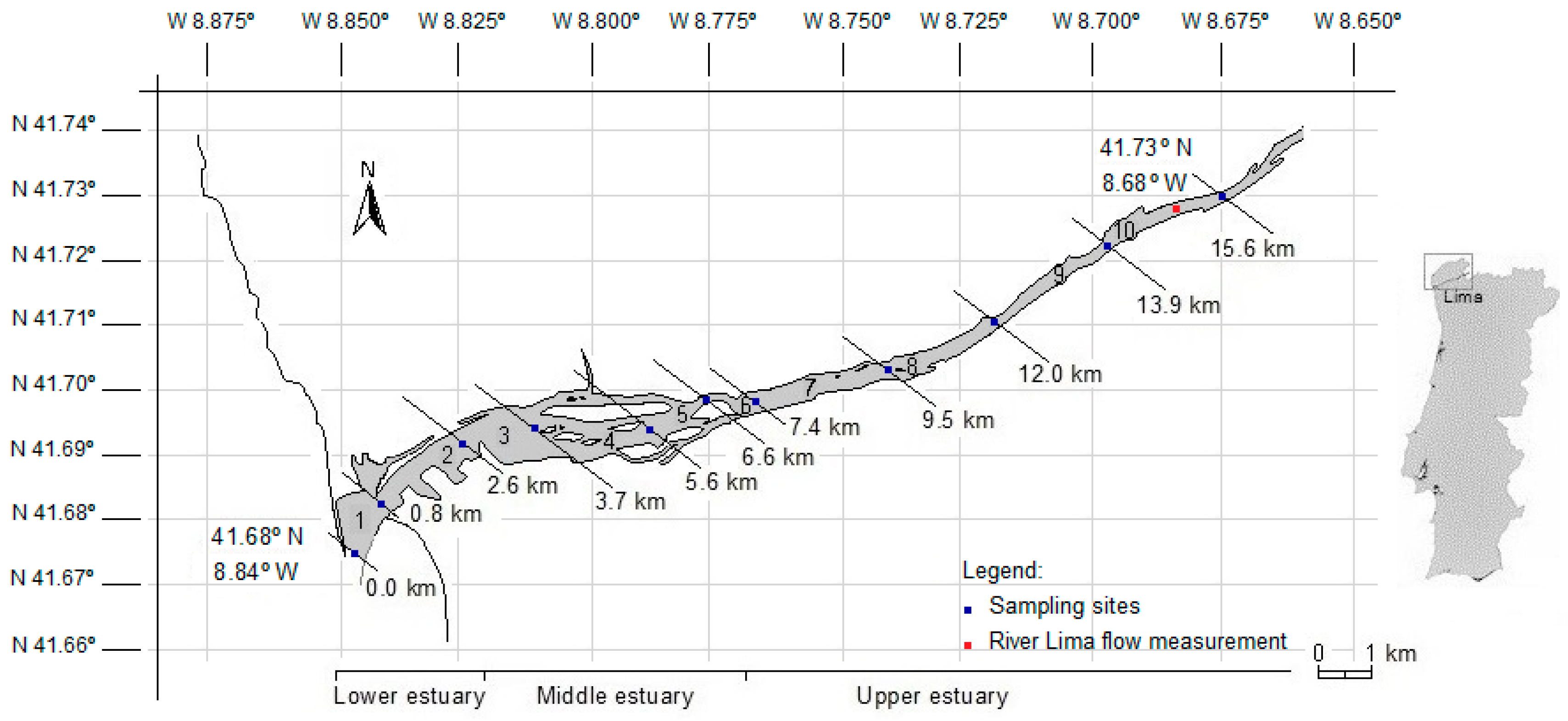
2.1. The Study Area
2.2. Sampling
2.3. Analytical Procedures
2.4. River Flow
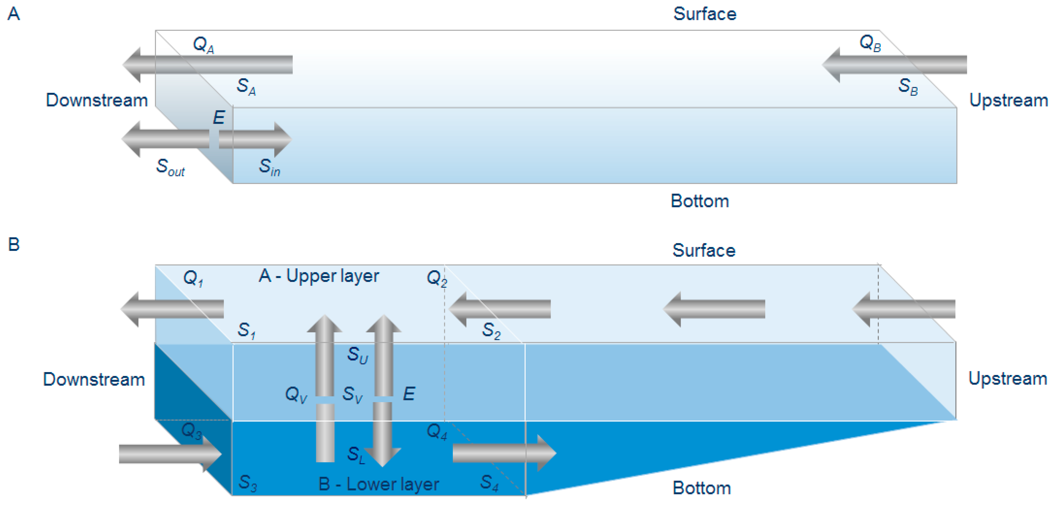
2.5. The Box Model
2.6. Data Analysis
3. Results
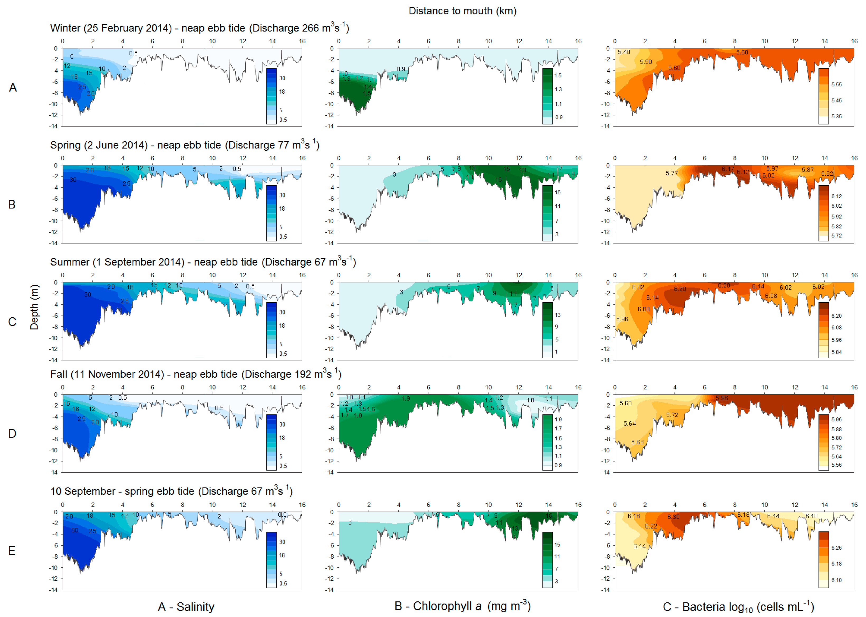
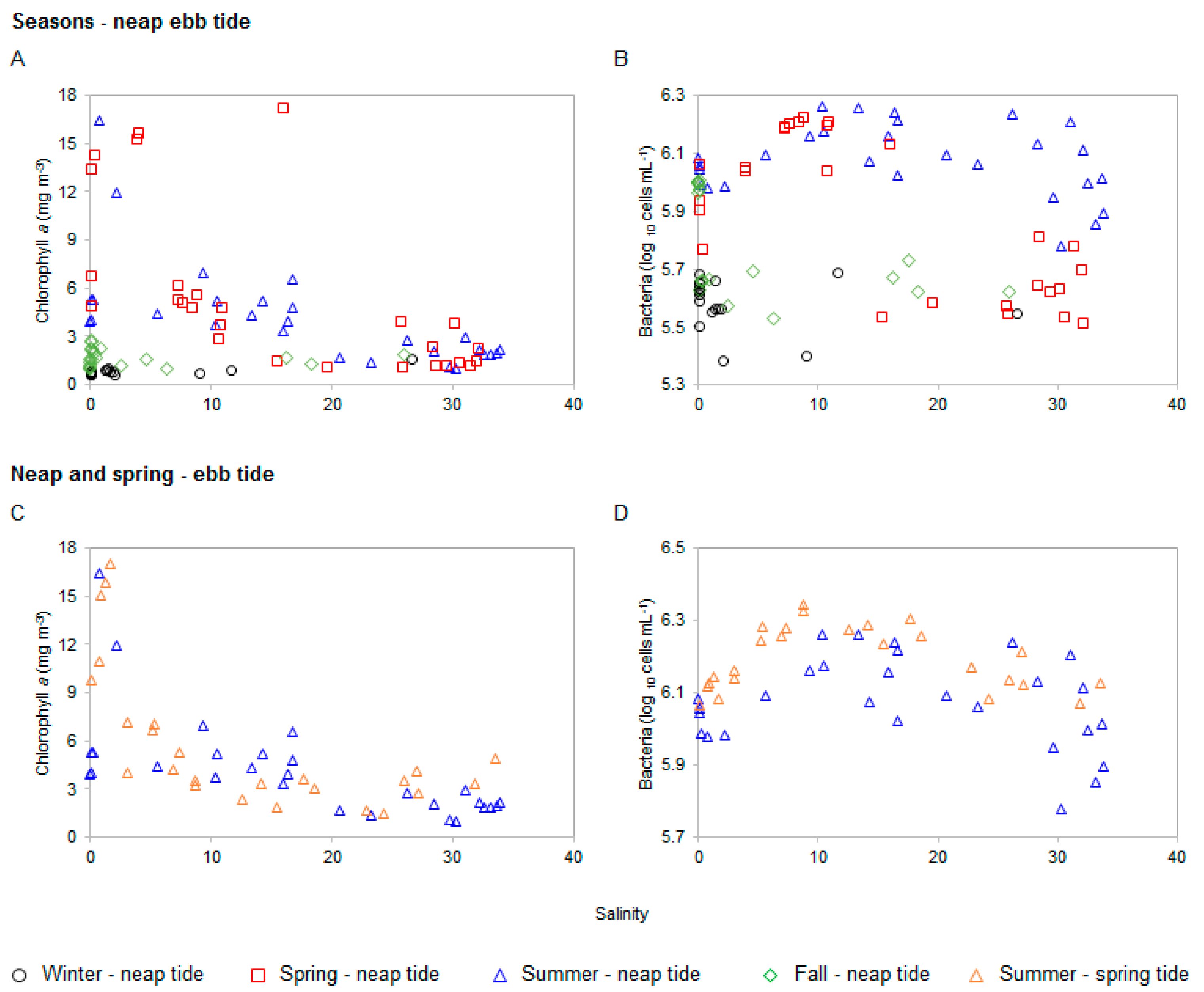
3.1. Bacteria and Chlorophyll a Profiles
3.2. Box Model
4. Discussion
4.1. Freshwater Inflow
4.2. Chlorophyll a and Bacteria Dynamics
4.3. Box Model Approach
5. Conclusions
Supplementary Materials
Author Contributions
Funding
Acknowledgments
Conflicts of Interest
References
- Jickells, T.D.; Andrewsa, J.E.; Parkes, D.J.; Suratman, S.; Aziz, A.A.; Hee, Y.Y. Nutrient transport through estuaries: The importance of the estuarine geography. Estuar. Coast. Shelf. Sci. 2014, 150, 215–229. [Google Scholar] [CrossRef]
- Robson, B.J.; Bukaveckas, P.A.; Hamilton, D.P. Modelling and mass balance assessments of nutrient retention in a seasonally-flowing estuary (Swan River Estuary, Western Australia). Estuar. Coast. Shelf Sci. 2008, 76, 282–292. [Google Scholar] [CrossRef]
- Saraiva, S.; Pina, E.P.; Martins, E.F.; Santos, E.M. Modelling the influence of nutrient loads on Portuguese estuaries. Hydrobiologia 2007, 587, 5–18. [Google Scholar] [CrossRef]
- Bordalo, A.A.; Vieira, M.E.C. Spatial variability of phytoplankton, bacteria and viruses in the mesotidal salt wedge Douro Estuary (Portugal). Estuar. Coast. Shelf Sci. 2005, 63, 143–154. [Google Scholar] [CrossRef]
- Wolanski, E.; Elliott, M. Estuarine Ecohydrology—An Introduction, 2nd ed.; Elsevier: Amsterdam, The Netherlands, 2016; pp. 1–87. ISBN 978-0-444-63398-9. [Google Scholar]
- Dyer, K.R. Estuaries. A Physical Introduction, 2nd ed.; John Wiley and Sons: Chichester, UK, 1997; ISBN 978-0-471-97471-0. [Google Scholar]
- Pritchard, D.W. Dispersion and flushing of pollutants in estuaries. Proc. Am. Soc. Civ. Eng. J. Hydraul. Div. 1969, 95, 115–124. [Google Scholar]
- Libes, S.M. Introduction to Marine Biogeochemistry, 2nd ed.; Elsevier Inc.: New York, NY, USA, 2009; pp. 65–100. ISBN 978-0-12-088530-5. [Google Scholar]
- Cloern, J. Tidal stirring and phytoplankton bloom dynamics in an estuary. J. Mar. Res. 1991, 49, 203–221. [Google Scholar] [CrossRef]
- Calbet, A.; Landry, M.R. Phytoplankton growth, microzooplankton grazing, and carbon cycling in marine systems. Limnol. Oceanogr. 2004, 49, 51–57. [Google Scholar] [CrossRef]
- Cermeño, P.; Maranon, E.; Pérez, V.; Serret, P.; Fernández, E.; Castro, C. Phytoplankton size structure and primary production in a highly dynamic coastal ecosystem (Ría de Vigo, NW-Spain): Seasonal and shorttime scale variability. Estuar. Coast. Shelf Sci. 2006, 67, 251–266. [Google Scholar] [CrossRef]
- Kimmerer, W.J. Effects of freshwater flow on abundance of estuarine organisms: Physical effects or trophic linkages? Mar. Ecol. Progr. Ser. 2002, 243, 39–55. [Google Scholar] [CrossRef]
- Azhikodan, G.; Yokoyama, K. Spatio-temporal variability of phytoplankton (Chlorophyll-a) in relation to salinity, suspended sediment concentration, and light intensity in a macrotidal estuary. Cont. Shelf Res. 2016, 126, 15–26. [Google Scholar] [CrossRef]
- Roegner, G. Hydrodynamic control of the supply of suspended chlorophyll a to infaunal estuarine bivalves. Estuar. Coast. Shelf Sci. 1998, 47, 369–384. [Google Scholar] [CrossRef]
- Valdes-Weaver, L.M.; Piehler, M.F.; Pinckney, J.L.; Howe, K.E.; Rossignol, K.; Paerl, H.W. Long-term temporal and spatial trends in phytoplankton biomass and class-level taxonomic composition in the hydrologically variable Neuse-Pamlico estuarine continuum, North Carolina U.S.A. Limnol. Oceanogr. 2006, 51, 1410–1420. [Google Scholar] [CrossRef]
- Chaudhuri, K.; Manna, S.; Sarma, K.S.; Naskar, P.; Bhattacharyya, S.; Bhattacharyya, M. Physicochemical and biological factors controlling water column metabolism in Sundarbans estuary, India. Aquat. Biosyst. 2012, 8, 1–16. [Google Scholar] [CrossRef] [PubMed]
- Hitchcock, J.N.; Mitrovic, S.M. Highs and lows: The effect of differently sized freshwater inflows on estuarine carbon, nitrogen, phosphorus, bacteria and chlorophyll a dynamics. Estuar. Coast. Shelf Sci. 2015, 156, 71–82. [Google Scholar] [CrossRef]
- Anderson, O.R. The role of heterotrophic microbial communities in estuarine C budgets and the biogeochemical C Cycle with implications for global warming: Research opportunities and challenges. J. Eukaryot. Microbiol. 2016, 63, 394–409. [Google Scholar] [CrossRef] [PubMed]
- Attermeyer, K.; Tittel, J.; Allgaier, M.; Frindte, K.; Wurzbacher, C.; Hilt, S.; Kamjunke, N.; Kamjunke, H. Effects of light and autochthonous carbon additions on microbial turnover of allochthonous organic carbon and community composition. Microb. Ecol. 2015, 69, 361–371. [Google Scholar] [CrossRef] [PubMed]
- Painchaud, J.; Lefaivre, D.; Therriault, J.C. Bacterial dynamics in the upper St. Lawrence estuary. Limnol. Oceanogr. 1996, 41, 1610–1618. [Google Scholar] [CrossRef]
- Mallin, M.A.; Williams, K.E.; Esham, E.C.; Lowe, R.P. Effect of human development on bacteriological water quality in coastal watersheds. Ecol. Appl. 2000, 10, 1047–1056. [Google Scholar] [CrossRef]
- INAG—Instituto da Água. Questões Significativas da Gestão da Água—Região Hidrográfica do Minho e Lima. 2009. Available online: http://dqa.inag.pt/dqa2002/port/p_dispos/QSigaPP/Questoes_Minho_Lima_30_01_2009.pdf (accessed on 16 December 2012).
- Vale, L.M.; Dias, J.M. The effect of tidal regime and river flow on the hydrodynamics and salinity structure of the Lima Estuary: Use of a numerical model to assist on estuary classification. J. Coast. Res. Spec. Issue 2011, 64, 1604–1608. [Google Scholar]
- Azevedo, I.; Ramos, S.; Mucha, A.P.; Bordalo, A.A. Applicability of ecological assessment tools for management decision-making: A case study from the Lima estuary (NW Portugal). Ocean Coast. Manag. 2013, 72, 54–63. [Google Scholar] [CrossRef]
- Almeida, C.M.R.; Mucha, A.P.; Vasconcelos, M.T. Role of different salt marsh plants on metal retention in an urban estuary (Lima estuary, NW Portugal). Estuar. Coast. Shelf Sci. 2011, 91, 243–249. [Google Scholar] [CrossRef]
- Parsons, T.R.; Maita, Y.; Lalli, C.M. A Manual of Chemical and Biological Methods for Seawater Analysis; Pergamon Press: Oxford, UK, 1984; 173p, ISBN 0-08-030288-2. [Google Scholar]
- SCOR-UNESCO. Determination of Photosynthtic Pigments in Sea Water. In Monographs on Oceanographic Methodology; UNESCO, Ed.; UNESCO Press: Paris, France, 1966; Volume 1, pp. 10–69. [Google Scholar]
- Porter, K.G.; Feig, Y.S. The use of DAPI for identifying and counting aquatic microflora. Limnol. Oceanogr. 1980, 41, 1610–1618. [Google Scholar]
- Herschy, R.W. Streamflow Measurement, 2nd ed.; E & FN Spon: London, UK, 1995; pp. 5–13. ISBN 978-0-41-919490-3. [Google Scholar]
- Venice System. Symposium on the classification of brackish waters, Venice, Italy, 8–14 April 1958. Arch. Oceanogr. Limnol. 1958, 11, 1–248. Available online: https://aslopubs.onlinelibrary.wiley.com/doi/abs/10.4319/lo.1958.3.3.0346 (accessed on 16 December 2012).
- European Union (EU). Directive 2000/60/EC of the European Parliament and of the Council of 23 October 2000 establishing a framework for community action in the field of water policy. Off. J. Eur. Union 2000, L327, 1–72. [Google Scholar]
- Robarts, R.D.; Zohary, T.; Waiserl, M.J.; Yacobi, Y.Z. Bacterial abundance, biomass, and production in relation to phytoplankton biomass in the Levantine basin of the southeastern Mediterranean Sea. Mar. Ecol. Prog. Ser. 1996, 137, 273–281. [Google Scholar] [CrossRef]
- Hofmeister, R.; Flöser, G.; Schartau, M. Estuary-type circulation as a factor sustaining horizontal nutrient gradients in freshwater-influenced coastal systems. Geo-Mar. Lett. 2017, 37, 179–192. [Google Scholar] [CrossRef]
- Iriarte, A.; Villate, F.; Uriarte, I.; Alberdi, L.; Intxausti, L. Dissolved oxygen in a temperate estuary: The influence of hydro-climatic factors and eutrophication at seasonal and inter-annual time scales. Estuaries Coast. 2015, 38, 1000–1015. [Google Scholar] [CrossRef]
- Carbone, M.E.; Spetter, C.V.; Marcovecchio, J.E. Seasonal and spatial variability of macronutrients and Chlorophyll a basead on GIS in the South American estuary (Bahía Blanca, Argentina). Environ. Earth Sci. 2016, 75, 1–13. [Google Scholar] [CrossRef]
- Gonçalves, D.A.; Marques, S.C.; Primo, A.L.; Martinho, F.; Bordalo, M.; Pardal, M.A. Mesozooplankton biomass and copepod estimated production in a temperate estuary (Mondego estuary): Effects of processes operating at different timescales. Zool. Stud. 2015, 54, 57. [Google Scholar] [CrossRef]
- Winder, M.; Cloern, J.E. The annual cycles of phytoplankton biomass. Phil. Trans. R. Soc. B 2010, 365, 3215–3226. [Google Scholar] [CrossRef] [PubMed]
- Buchan, A.; LeCleir, G.R.; Gulvik, C.A.; González, J.M. Master recyclers: Features and functions of bacteria associated with phytoplankton blooms. Nat. Rev. Microbiol. 2014, 12, 686–698. [Google Scholar] [CrossRef] [PubMed]
- Barrio, P.; Ganju, N.K.; Aretxabaleta, A.L.; Hayn, M.; García, A.; Howarth, R.W. Modeling future scenarios of light attenuation and potential seagrass success in a eutrophic estuary. Estuar. Coast. Shelf Sci. 2014, 149, 13–23. [Google Scholar] [CrossRef]
- Lu, Z.; Gan, J. Controls of seasonal variability of phytoplankton blooms in the Pearl river estuary. Deep Sea Res. Part II Top. Stud. Oceanogr. 2015, 17, 86–96. [Google Scholar] [CrossRef]
- Bukaveckas, P.A.; Barry, L.E.; Beckwith, M.J.; David, V.; Lederer, B. Factors determining the location of the chlorophyll maximum and the fate of algal production within the tidal freshwater James river. Estuaries Coast. 2011, 34, 569–582. [Google Scholar] [CrossRef]
- Fisher, T.R.; Harding, L.W., Jr.; Stanley, D.W.; Ward, L.G. Phytoplankton, nutrients, and turbidity in the Chesapeake, Delaware, and Hudson estuaries. Estuar. Coast. Shelf Sci. 1988, 27, 61–93. [Google Scholar] [CrossRef]
- Desmit, X.; Ruddick, K.; Lacroix, G. Salinity predicts the distribution of chlorophyll a spring peak in the southern North Sea continental waters. J. Sea Res. 2015, 103, 59–74. [Google Scholar] [CrossRef]
- Selje, N.; Simon, M. Composition and dynamics of particle-associated and free-living bacterial communities in the Weser estuary, Germany. Aquat. Microb. Ecol. 2003, 30, 221–237. [Google Scholar] [CrossRef]
- Bacelar-Nicolau, P.; Nicolau, L.B.; Marques, J.C.; Morgado, F.; Pastorinho, R.; Azeiteiro, U.M. Bacterioplankton dynamics in the Mondego estuary (Portugal). Acta Oecol. 2003, 24, S67–S75. [Google Scholar] [CrossRef]
- Hobbie, J.E. A comparison of the ecology of planktonic bacteria in fresh and salt water. Limnol. Oceanogr. 1988, 33, 750–764. [Google Scholar]
- Munro, P.M.; Gauthier, M.J.; Breittmayer, V.A.; Bonjiovanni, J. Influence of osmoregulation processes on starvation survival of Escherichia coli in seawater. Appl. Env. Microbiol. 1989, 55, 121–124. [Google Scholar]
- Bordalo, A.A. Microbiological water quality in urban coastal beaches: The influence of water dynamics and optimization of the sampling strategy. Water Res. 2003, 37, 3233–3241. [Google Scholar] [CrossRef]
- Bunse, C.; Bertos-Fortis, M.; Sassenhagen, I.; Sildever, S.; Sjöqvist, S.; Godhe, A.; Gross, S.; Kremp, A.; Lips, I.; Lundholm, N.; et al. Spatio-temporal interdependence of bacteria and phytoplankton during a Baltic Sea spring bloom. Front. Microbiol. 2016, 7, 517. [Google Scholar] [CrossRef] [PubMed]
- Campbell, B.; Kirchman, D.L. Bacterial diversity, community structure and potential growth rates along an estuarine salinity gradient. ISME J. 2013, 7, 210–220. [Google Scholar] [CrossRef] [PubMed]
- Xia, X.; Guo, W.; Liu, H. Dynamics of the bacterial and archaeal communities in the Northern South China Sea revealed by 454 pyrosequencing of the 16S rRNA gene. Deep Sea Res. Part II Top. Stud. Oceanogr. 2015, 117, 97–107. [Google Scholar] [CrossRef]
- Herlemann, D.P.R.; Lundin, D.; Andersson, A.F.; Labrenz, M.; Jürgens, K. Phylogenetic signals of salinity and season in bacterial community composition across the salinity gradient of the Baltic Sea. Front. Microbiol. 2016, 7, 1883. [Google Scholar] [CrossRef]
- Ducklow, H.W.; Schultz, G.; Raymond, P.; Bauer, J.; Shiah, F.K. Bacterial Dynamics in Large and Small Estuaries. In Microbial Ecology of Estuaries, Proceedings of the 8th International Symposium on Microbial Ecology, Halifax, NS, Canada, 9–14 August 1998; Bell, C.R., Brylinsky, M., Johnson-Green, P., Eds.; Atlantic Canada Society for Microbial Ecology: Halifax, NS, Canada, 1999; pp. 105–111. [Google Scholar]
- Testa, J.M.; Kemp, W.M. Variability of biogeochemical processes and physical transport in a partially stratified estuary: A box-modelling analysis. Mar. Ecol. Prog. Ser. 2008, 356, 63–79. [Google Scholar] [CrossRef]
- Lyngsgaard, M.M.; Markager, S.; Richardson, K.; Møller, E.F.; Jakobsen, H.H. How well does chlorophyll explain the seasonal variation in phytoplankton activity? Estuaries Coast. 2017. [Google Scholar] [CrossRef]
- Martinez, E.; Antoine, D.; D’Ortenzio, F.; Montégut, C.B. Phytoplankton spring and fall blooms in the North Atlantic in the 1980s and 2000s. J. Geophys. Res. 2011, 116, 1–11. [Google Scholar] [CrossRef]
- Van Alstyne, K.L.; Nelson, T.A.; Ridgway, R.L. Environmental chemistry and chemical ecology of ‘‘green tide’’ seaweed blooms. Integr. Comp. Biol. 2015, 55, 518–532. [Google Scholar] [CrossRef]
- Liu, W.C.; Chan, W.T. Assessment of climate change impacts on water quality in a tidal estuarine system using a three-dimensional model. Water 2016, 8, 60. [Google Scholar] [CrossRef]
- Kara, E.; Shade, A. Temporal dynamics of south end tidal creek (Sapelo Island, Georgia) bacterial communities. Appl. Environ. Microbiol. 2009, 75, 1058–1064. [Google Scholar] [CrossRef] [PubMed]
- Wan, Y.; Qiu, C.; Doering, P.; Ashton, M.; Sun, D.; Coley, T. Modeling residence time with a three-dimensional hydrodynamic model: Linkage with chlorophyll a in a subtropical estuary. Ecol. Model. 2013, 268, 93–102. [Google Scholar] [CrossRef]
- Vallières, C.; Retamal, L.; Ramlal, P.; Osburn, C.L.; Vincent, W.F. Bacterial production and microbial food web structure in a large arctic river and the coastal Arctic Ocean. J. Mar. Syst. 2008, 74, 756–773. [Google Scholar] [CrossRef]
- Crump, B.C.; Hopkinson, C.S.; Sogin, M.L.; Hobbie, J.E. Microbial biogeography along an estuarine salinity gradient: Combined influences of bacterial growth and residence time. Appl. Environ. Microbiol. 2004, 70, 1494–1505. [Google Scholar] [CrossRef]
- Hoch, M.P.; Kirchman, D.L. Seasonal and inter-annual variability in bacterial production and biomass in a temperate estuary. Mar. Ecol. Prog. Ser. 1993, 98, 83–295. [Google Scholar] [CrossRef]
- Hulot, F.D.; Morin, P.J.; Loreau, M. Interactions between algae and the microbial loop in experimental microcosms. Oikos 2001, 95, 231–238. [Google Scholar] [CrossRef]
- Martinussen, I.; Thingstad, T.F. Utilization of N, P and organic C by heterotrophic bacteria. II. Comparison of experiments and a mathematical model. Mar. Ecol. Prog. Ser. 1987, 37, 285–293. [Google Scholar] [CrossRef]


| Salt Water Stretch | ||||||
|---|---|---|---|---|---|---|
| Season | Concentration Range | Freshwater | Oligohaline | Mesohaline | Polyhaline | Seawater |
| Winter | Chlorophyll a (mg m−3) | 0.57–0.75 | 0.57–1.00 | 0.66–0.91 | 1.58 | - |
| Bacteria (log10 cells mL−1) | 5.50–5.68 | 5.38–5.66 | 5.40 | 5.55 | - | |
| Spring | Chlorophyll a (mg m−3) | 4.90–14.30 | 15.24–15.69 | 1.50–6.20 | 1.13–3.95 | 1.14–3.83 |
| Bacteria (log10 cells mL−1) | 5.77–6.06 | 6.04–6.05 | 5.53–6.23 | 5.55–5.81 | 5.52–5.78 | |
| Summer | Chlorophyll a (mg m−3) | 3.88–5.30 | 11.95–16.50 | 3.37–6.93 | 1.05–2.72 | 0.96–2.92 |
| Bacteria (log10 cells mL−1) | 5.99–6.08 | 5.98 | 6.02–6.26 | 5.95–6.24 | 5.78–6.21 | |
| Fall | Chlorophyll a (mg m−3) | 0.96–2.72 | 1.22–2.27 | 0.96–1.67 | 1.30–1.92 | - |
| Bacteria (log10 cells mL−1) | 5.63–6.00 | 5.57–5.69 | 5.53–5.73 | 5.62 | - | |
| Summer (spring tide) | Chlorophyll a (mg m−3) | 9.78 | 7.13–17.04 | 1.86–7.02 | 1.50–4.16 | 3.37–4.87 |
| Bacteria (log10 cells mL−1) | 6.06 | 6.09–6.16 | 6.23–6.35 | 6.08–6.26 | 6.07–6.13 | |
| Generation Time (h) | ||||||
|---|---|---|---|---|---|---|
| Winter | Spring | Summer | Fall | |||
| Estuary Stretch | Box | Neap Tide | Neap Tide | Neap Tide | Spring Tide | Neap Tide |
| Lower estuary | box 1A | - | - | 1.55 | 12.32 | - |
| box 1B | - | 2.82 | - | 22.13 | - | |
| box 2A | 6.95 | 5.97 | 3.48 | 4.56 | 10.16 | |
| box 2B | - | 16.52 | - | - | ||
| Middle estuary | box 3 | - | - | - | - | 53.56 |
| box 3A | - | - | 6.81 | 27.43 | - | |
| Box 4 | 101 | - | - | - | ||
| box 4A | - | 2.01 | 5.90 | 22.40 | - | |
| box 5 | - | 211 | - | - | 1.80 | |
| box 6 | - | - | 16.47 | - | 11.23 | |
| Upper estuary | box 7 | 6.19 | - | - | - | - |
| Box 8 | 64.55 | - | - | - | 64.29 | |
| box 9 | - | 10.40 | 17.41 | - | - | |
| box 10 | - | 10.80 | 24.86 | - | - | |
© 2019 by the authors. Licensee MDPI, Basel, Switzerland. This article is an open access article distributed under the terms and conditions of the Creative Commons Attribution (CC BY) license (http://creativecommons.org/licenses/by/4.0/).
Share and Cite
Fernandes, É.; Teixeira, C.; Bordalo, A.A. Coupling between Hydrodynamics and Chlorophyll a and Bacteria in a Temperate Estuary: A Box Model Approach. Water 2019, 11, 588. https://doi.org/10.3390/w11030588
Fernandes É, Teixeira C, Bordalo AA. Coupling between Hydrodynamics and Chlorophyll a and Bacteria in a Temperate Estuary: A Box Model Approach. Water. 2019; 11(3):588. https://doi.org/10.3390/w11030588
Chicago/Turabian StyleFernandes, Élia, Catarina Teixeira, and Adriano A. Bordalo. 2019. "Coupling between Hydrodynamics and Chlorophyll a and Bacteria in a Temperate Estuary: A Box Model Approach" Water 11, no. 3: 588. https://doi.org/10.3390/w11030588
APA StyleFernandes, É., Teixeira, C., & Bordalo, A. A. (2019). Coupling between Hydrodynamics and Chlorophyll a and Bacteria in a Temperate Estuary: A Box Model Approach. Water, 11(3), 588. https://doi.org/10.3390/w11030588