Impact of Climate Variability on Blue and Green Water Flows in the Erhai Lake Basin of Southwest China

Abstract

The Erhai Lake Basin is a crucial water resource of the Dali prefecture. This research used the soil and water assessment tool (SWAT) and the China Meteorological Assimilation Driving Datasets for the SWAT model (CMADS) to estimate blue and green water flows. Then the spatial and temporal change of blue and green water flows was investigated. With the hypothetical climate change scenarios, the sensitivity of blue and green water flows to precipitation and temperature has also been analyzed. The results showed that: (1) The CMADS reanalysis dataset can capture the observed probability density functions for daily precipitation and temperature. Furthermore, the CMADS performed well in monthly variables simulation with relative bias and absolute bias less than 7% and 0.5 °C for precipitation and temperature, respectively; (2) blue water flow has increased while green water flow has decreased during 2009 to 2016. The spatial distribution of blue water flow was uneven in the Erhai Lake Basin with the blue water flow increased from low altitudes to mountain areas. While the spatial distribution of green water flow was more homogeneous; (3) a 10% increase in precipitation can bring a 20.8% increase in blue water flow with only a 2.5% increase in green water flow at basin scale. When temperature increases by a 1.0 °C, the blue water flow and green water flow changes by −3% and 1.7%, respectively. Blue and green water flows were more sensitive to precipitation in low altitude regions. In contrast, the water flows were more sensitive to temperature in the mountainous area.

1. Introduction

The water resources availability has been affected by climate variability in the past decades, which has caused sustainability concerns in many parts of the world [1,2]. Previous studies have reported that climate variability can alter precipitation, evapotranspiration, soil water, and runoff [3,4,5] resulting in freshwater resources redistributing in spatial and temporal dimensions [6,7]. With warmer climate conditions, the water-holding capacity of the atmosphere has been increasing, and as a result, the hydrological cycle will be intensified [8,9] posing more challenges to water resource management. Therefore, it is necessary to investigate the impact of climate variability on freshwater resources, which will assist policymakers and administrators to manage water resources in the context of climate change. In general, blue water, namely the surface and groundwater runoff directly generated from precipitation, has been emphasized by water resources assessment and management studies. While green water, including actual evapotranspiration and soil water, has often been ignored [10]. In fact, green water plays an important role in rain-fed crop production and ecosystem services provision [11,12]. According to the study by Liu et al., more than 80% of the water consumption for global crop production is supported by green water [13]. Natural terrestrial ecosystems, such as grasslands and forests, depend almost entirely on green water [14]. So green water is critical for maintaining the productivity and serviceability of the terrestrial ecosystem. However, in traditional water resources assessment, only the available water resource was taken into consideration. Limitations such as this should be addressed, and temporal–spatial variation should be explored to provide scientific evidence for the construction of water resources management modes and systems.

The Erhai Lake Basin in Southwest China is not only an ecologically fragile area but also a vulnerable area from climate change. As the effects of climate change become more serious, the imbalance between the supply and demand of water resources in the Erhai Lake Basin will be more prominent [15,16]. Thus, it is necessary to assess the impact of climate change on water resources in the Erhai Lake Basin. In the previous studies, the variation of water resources in the Erhai Lake Basin has been analyzed. However, most of the researches focus on the impact of precipitation variations on annual runoff [17,18]. In fact, temperature is also a main factor influencing water resources. The land surface evaporation and water consumption of crops will increase as the temperature rises, leading to a change in water resources [19]. In addition, green water resources should also be considered in this ecologically fragile area. Given the above, the investigation of spatio–temporal distribution characteristics of blue and green water resources is useful for water resources planning and ecological protection in the Erhai Lake Basin.

The concept of blue and green water resources was first proposed by Falkenmark [20]. Since then, numerous methods have been used to assess blue water and green water resources. With the development of distributed hydrological models, the temporal–spatial variations of blue and green water resources can be estimated by methods which have a clearer physical mechanism [11,21,22,23]. It has been demonstrated that the soil and water assessment tool (SWAT) model can simulate blue and green water resources and detect the impacts of climate variability on hydrological components [24,25,26,27]. However, in the basins where the conventional in situ data are not available, the distributed physically-based model cannot estimate the hydrological processes as there are insufficient weather gauges. The satellite-based precipitation datasets, such as Tropical Rainfall Measuring Mission (TRMM) 3B42V7 and the Precipitation Estimation from Remotely Sensed Information using Artificial Neural Networks- Climate Data Record (PERSIANN-CDR), can be used as the forcing data for hydrological models. Nevertheless, the errors would result from measure, resample and retrieval algorithm [28,29,30]. It has been proved that the reanalysis datasets obtained from observed data and model forecast performance better than satellite-based precipitation [31]. The China Meteorological Assimilation Driving Datasets for the SWAT model (CMADS) developed by Dr. Xianyong Meng from China Agriculture University (CAU) is one of the available reanalysis datasets. This dataset provides multiple meteorological elements with resolutions of 1/3°, 1/4°, 1/8°, and 1/16° and can be used to drive various hydrological models [32,33]. Many previous studies have shown that the CMADS reanalysis dataset has a high accuracy for weather element simulation and has been widely used in East Asia, including Heihe River Basin (China), Juntanghu River basin (China), Lijiang River Basin (China), Han River Basin (Korean Peninsula), and so on [34,35,36,37,38,39,40,41,42,43,44]. Based on the above analysis, the CMADS reanalysis dataset and SWAT model can be considered as the important basic data and simulation tool for investigating the impact of climate variability on blue and green water resources in ungauged basins (e.g., Erhai River Basin).

This research selected Erhai River Basin as the study area, and the impact of climate variability on blue and green water flows has been analyzed by the SWAT model and hypothetical climate change scenarios. The remaining sections of this paper are organized as follows: The study area, modeling approach (blue and green water flows simulation based on SWAT model), dataset and hypothetical climate change scenarios are introduced in Section 2; Section 3 shows the evaluation of CMADS reanalysis dataset and SWAT model, spatial and temporal variability of blue and green water flows in the recent eight years, sensitivity of blue and green water flows to climate change; and the discussion and conclusions are summarized in Section 4 and Section 5.

2. Materials and Methods

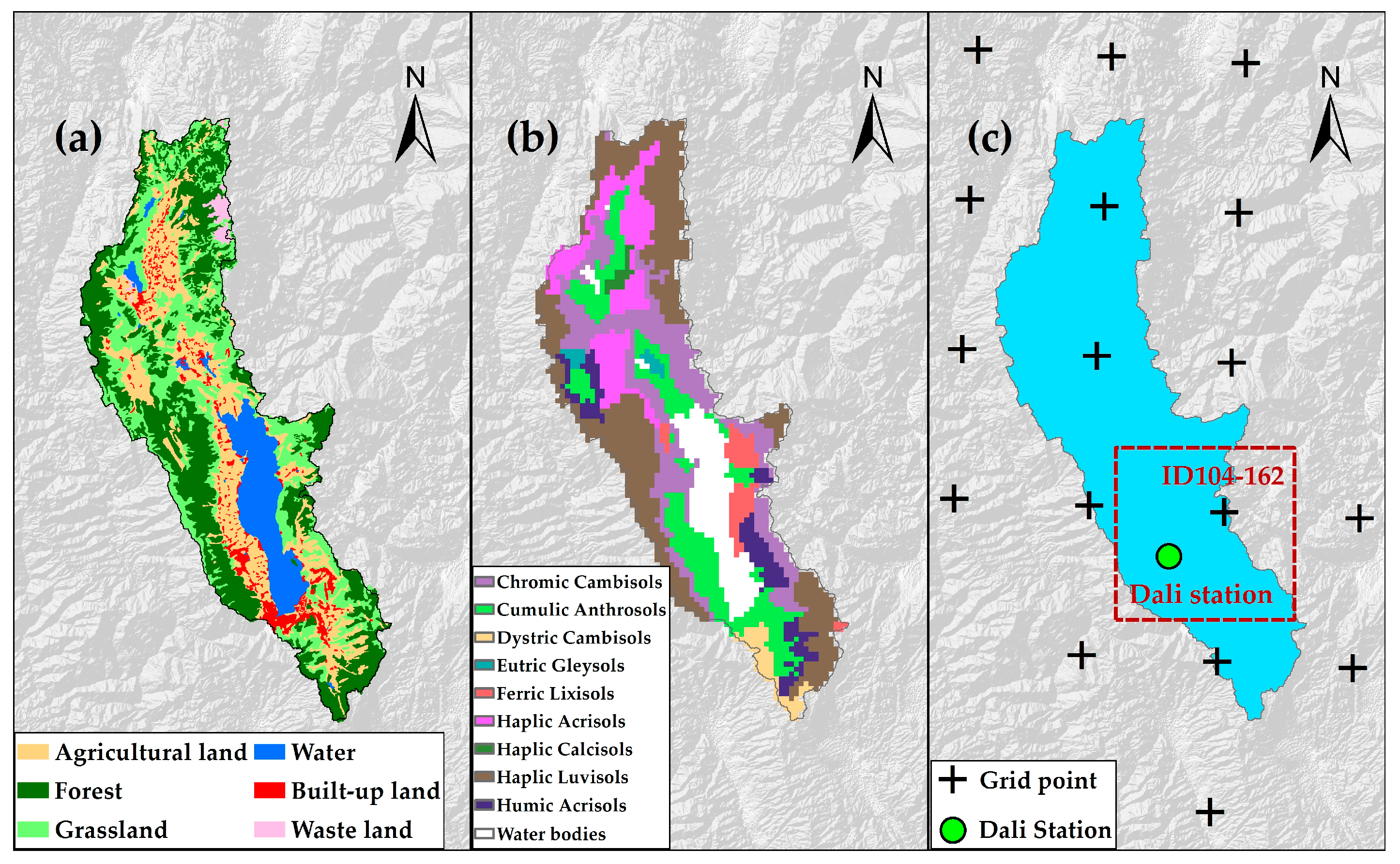
2.1. Study Area

The Erhai Lake Basin (ELB), situated between 99°50′ E and 100°27′ E and between 25°26′ N and 26°26′ N, is the area investigated in this study. The total area is 2496.6 km², accounting for 8.8% of the total area of the Dali prefecture. The elevation of the study area varies from 1958 to 4072 m with an average of 2458 m, dropping off from the edges of the basin to the center (Figure 1). The annual mean precipitation of ELB is about 850 mm with more than 85% falling from May to October. The climate is wetter in the west side, known locally as the famous Eighteen Streams Region, with an annual precipitation of 1072 mm and runoff of more than 200 mm. While on the Eryuan plain, the north side of the ELB, the annual precipitation drops to about 763 mm and the runoff is less than 100 mm. The weather in the basin is mild, with an annual average temperature of 16 °C [45,46].

Impacted by global warming and many other factors, the ELB has witnessed a series of eco–environmental issues, such as reduction in the lake water level, shortage of water resources, and a conflict between water supply and demand. Therefore, an accurate evaluation of water resources in the ELB is essential for water resources planning and management in the Dali prefecture.

2.2. Modeling Approach

The SWAT Model was used to quantify the water flows, including blue water flow (BWF) and green water flow (GWF) in this study. According to the study by Schuol et al. [11], BWF is the river discharge and the deep aquifer recharge, whereas GWF is represented by actual evapotranspiration (Figure 2). All these variables can be simulated by the SWAT Model. In addition, the green water coefficient (GWC) was used to account for the relative importance of BWF and GWF, which can be written as GWC = GWF/(BWF + GWF) [13].

The ArcSWAT 2012 is used for the model setup and parameterization. In this study, the ELR was divided into 151 sub-basins with a threshold drainage area of 10 km² and further into 722 hydrological response units (HRUs) based on the elevation, land use, and soil type. The monthly hydrological processes were simulated by the SWAT model. The entire simulation period covers 9 years (2008–2016), including a warming up period (2008), calibration period (2009–2014), and validation period (2015–2016). The model’s performance of simulating monthly discharge was quantified by the Nash–Sutcliffe values (E_NS), determination coefficient (R²) and relative error (RE) [47,48].

$$E_{NS}=1-\frac{{\displaystyle \sum _{i=1}^n\left(Q{o}_i-Q{s}_i\right)}}{{\displaystyle \sum _{i=1}^n\left(Q{o}_i-\overline{Q{o}_i}\right)}}$$

(1)

$$R^2=\frac{{\left[{\displaystyle \sum _{i=1}^n\left(Q{s}_i-\overline{Q{s}_i}\right){\displaystyle \sum _{i=1}^n\left(Q{o}_i-\overline{Q{o}_i}\right)}}\right]}^2}{{\displaystyle \sum _{i=1}^n{\left(Q{s}_i-\overline{Q{s}_i}\right)}^2}{\displaystyle \sum _{i=1}^n{\left(Q{o}_i-\overline{Q{o}_i}\right)}^2}}$$

(2)

$$RE=\left(\frac{\overline{Qs}-\overline{Qo}}{\overline{Qo}}\right)\times 100\%$$

(3)

where, Qo_i and Qs_i are observed discharge and simulated discharge respectively; $\overline{Qo}$ and $\overline{Qs}$ are the average value of observed discharge and simulated discharge respectively; n is the number of observed values. The higher E_NS and R² and the smaller RE, the better the model performance. According to the suggestion by Kumar and Merwade, the monthly discharge simulations with E_NS > 0.5 and RE < ±15% are acceptable simulations [49].

2.3. Data Sets and Evaluation

The basic data for model setup contains the digital elevation model (DEM), land use, soil, and weather. In this study, the Shuttle Radar Topography Mission (SRTM) 30 m digital elevation data was used for watershed delineation, which was provided by the Advanced Spaceborne Thermal Emission and Reflection Radiometer (Figure 1). The land use map in 2015 for this study was obtained from the Resource and Environment Data Cloud Platform (RESDC, http://www.resdc.cn/) (Figure 3a). The soil data was obtained from the China Soil Data Set (v1.1), based on the World Soil Database (HSDW) (http://westdc.westgis.ac.cn) (Figure 3b). The above data were used for HRU definition. The daily weather data were collected from the China Meteorological Assimilation Driving Datasets for the SWAT model (CMADS, http://www.cmads.org/) (Figure 3c). The CMADS V1.1 dataset is available from 2008 to 2016 with 0.25° spatial resolution (260 × 400 grid points). This dataset provides the daily max/min-temperatures, 24 h precipitation, solar radiation, air pressure, relative humidity, and wind speed which can be used to initialize SWAT models directly [32]. A total of 17 grid points within and around the ELB were used for the establishment of weather databases in this study. The CMADS V1.1 dataset has been assessed by weather station data collected in Dali station (location is shown as a green dot in Figure 3c). According to the data provided by National Meteorological Information Center (NMIC, http://data.cma.cn/), there is only one meteorological station, Dali, in the study area. Thus, the spatial distribution characteristics of Erhai Lake Basin cannot be fully represented. However, by using the grid data provided by CMADS, this problem can be well solved.

To evaluate the precipitation and temperature provided by the CMADS V1.1, we compared this reanalysis datasets (ID104-162) with the observed precipitation and temperature in the Dali station. This comparison was based on two temporal scales, namely daily scale and monthly scale. In the daily scale, a probability density functions (PDFs)-based assessment was used to illustrate the similarity between observed-PDF and simulated-PDF (Figure 4). An alternative metric-skill score (SS) was defined as Equation (4), which is greater than 0 and smaller than 1. When SS is close to 1, it means that the simulated-PDF fits perfectly with the observed-PDF [50]. At the monthly scale, the bias (B) or absolute bias (B_abs) and correlation coefficient (C) were used to evaluate the monthly precipitation and temperature (Equation (5) to Equation (7)) [51].

$$SS={\displaystyle \sum _1^n\min \left(F{s}_n,F{o}_n\right)}$$

(4)

where, n stands for the number of bins; Fs_n stands for the frequency of values in a given bin from the CMADS; and Fo_n stands for the frequency of values in a given bin from the observed data (Gauge). Summing up the minimum frequency values over all bins and then SS can be obtained.

$$R=\left(\frac{\overline{P_s}-\overline{P_o}}{\overline{P_o}}\right)\times 100\%$$

(5)

$$B_{abs}=\overline{T_s}-\overline{T_o}$$

(6)

$$C=\frac{Cov\left(V_s,V_o\right)}{\sqrt{Var\left(V_s\right)Var\left(V_s\right)}}$$

(7)

where $\overline{P_o}$ and $\overline{P_s}$ are the temporal average of observed precipitation and simulated precipitation, respectively; $\overline{T_o}$ and $\overline{T_s}$ are the temporal average of observed temperature and simulated temperature, respectively; $V_o$ and $V_s$ are the observed value (precipitation or temperature) and simulated value, respectively.

2.4. Climate Change Scenarios and Sensitivity Analysis

The sensitivity of water flows to climate variability can be considered as the proportional change of simulated BWF and GWF comparing with the observed values in the hypothetical climate change scenarios. According to this, the sensitivity can be calculated as follow:

$$\delta \left(WF,P\right)=\frac{f\left(P+\Delta P,T\right)-f\left(P,T\right)}{f\left(P,T\right)}\times 100\%$$

(8)

$$\delta \left(WF,T\right)=\frac{f\left(P,T+\Delta T\right)-f\left(P,T\right)}{f\left(P,T\right)}\times 100\%$$

(9)

where $\delta \left(WF,P\right)$ and $\delta \left(WF,T\right)$ are the response of water flow to precipitation change and temperature change; P and T are observed precipitation and observed temperature; $\Delta P$ and $\Delta T$ are the change of precipitation and temperature in the hypothetical climate change scenarios. In this study, we assumed that the precipitation in each grid point change by −30% to 30% with an interval of 10% and the temperature in each grid point change by −3 °C to +3 °C with an interval of 1 °C.

The Equation (8) and Equation (9) can be used to analyze the basin scale BWF and GWF variation in different precipitation and temperature scenarios. To compare the variation of sensitivity to climate change in different regions, a sensitivity index (SI) is designed in this study to express the change rate between BWF or GWF with precipitation and temperature. The relationship between water flow and precipitation/temperature can be described as:

$$\widehat{y}=ax+b.$$

(10)

where, $\widehat{y}$ is the simulated BWF or GWF; x is the precipitation or temperature; a and b are the coefficients, which can be estimated by the least square method. Then the SI can be calculated as:

$$SI=\frac{a}{WF}$$

(11)

where, WF is the multi-year average BWF or GWF of each sub-basin in current climate. The SI stands for the variation (%) of BWF or GWF as precipitation changes for 1% or temperature changes for 1 °C in each sub-basin. By comparing SI in different sub-basins, the difference of BWF and GWF’s response to climate change in different regions can be obtained.

3. Results

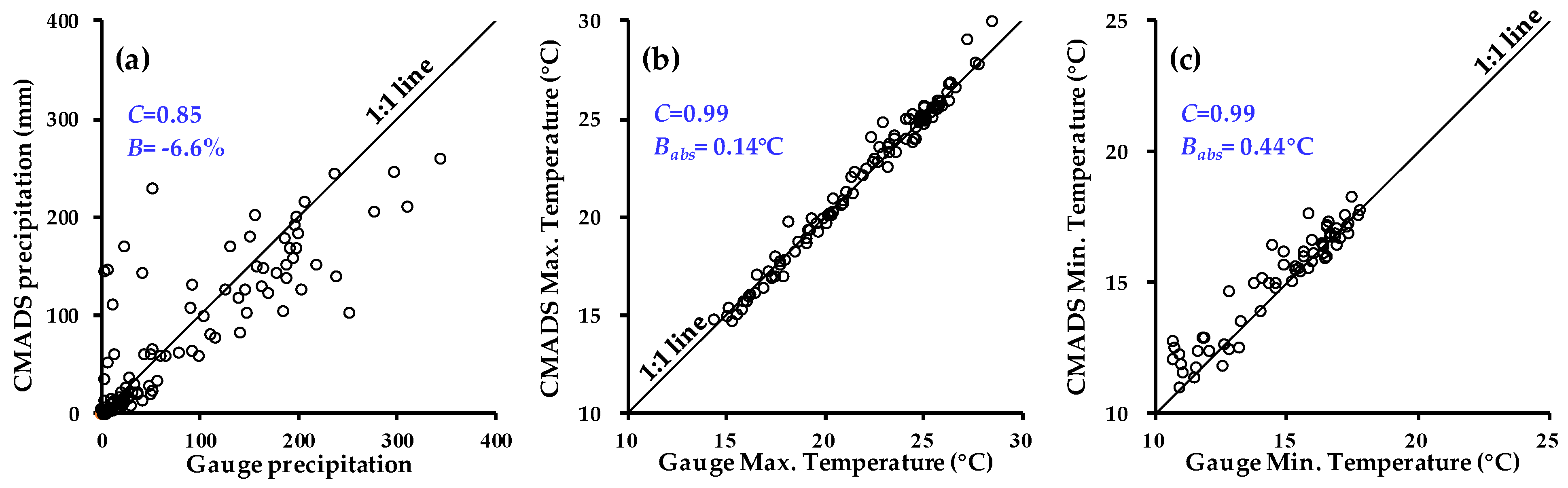
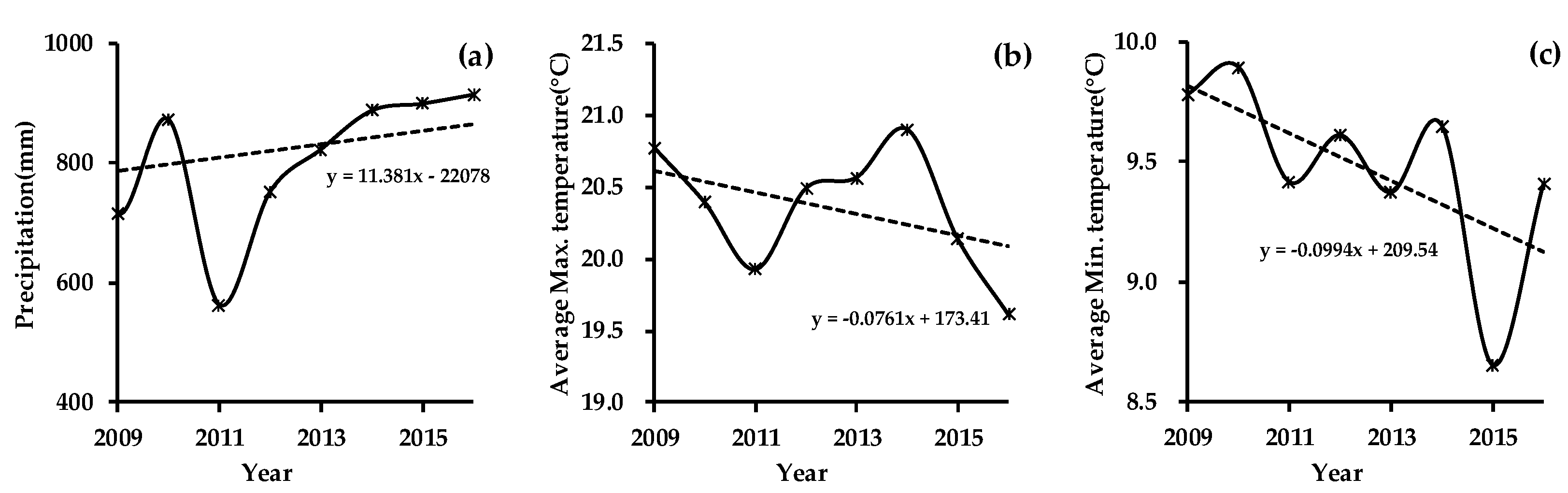
3.1. Evaluation of CMADS Precipitation and Temperature

Statistical results of CMADS reanalysis data and gauge observations (Dali Station) on daily scale and monthly scale are illustrated in Figure 5 and Figure 6. It can be found that the PDFs of CMADS reanalysis daily temperature are quite tightly clustered around the PDFs of gauge observations. The skill in the CMADS reanalysis Maximum temperature and Minimum temperature were higher than 0.95. CMADS tends to overestimate the amount of drizzle but did quite well for precipitation of more than 4 mm/day. The skill score for daily precipitation approaches 0.8 (Figure 5a). In general, the CMADs showed considerable skill in representing the PDFs of daily gauge observations. The monthly CMADS precipitation and temperature were highly consistent with the monthly gauge observations. In particular, the C values of monthly Maximum temperature and Minimum temperature were nearly 1.0. The relative bias ratio of monthly precipitation was less than 7% and the absolute biases of monthly Maximum temperature and Minimum temperature were less than 0.5 °C (Figure 6). Therefore, the CMADS reanalysis dataset can be used for hydrology process simulation in the ELB.

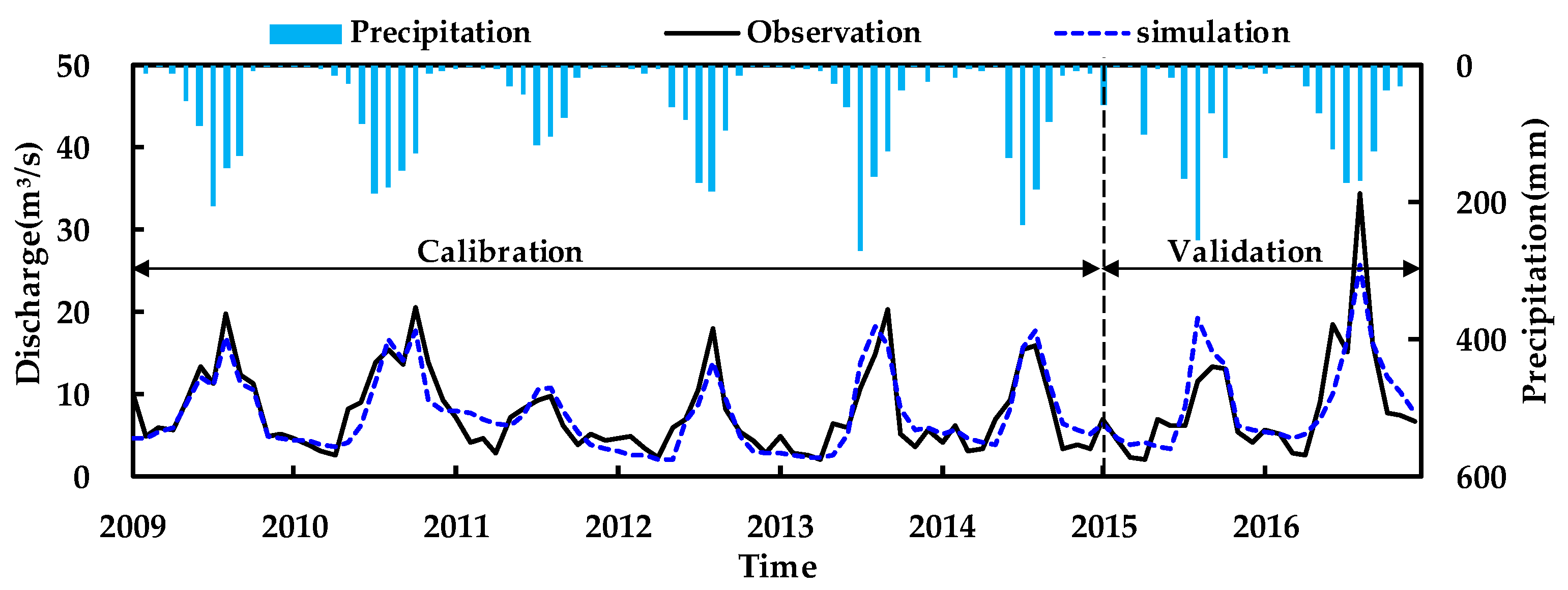
3.2. Evaluation of SWAT Simulation

The observed and SWAT simulated monthly streamflow at Liancheng Station from 2009 to 2016 is illustrated in Figure 7 (the statistical measures are provided in

Table 1. The calibration and validation statistics.

Period	ENS	R2	RE (%)
Calibration (2009 to 2014)	0.802	0.808	−3.7
Validation (2015 to 2016)	0.751	0.754	2.9

). It can be found that the simulated streamflow matched well with the observed streamflow except in a few months. E_NS and R² values were greater than 0.75 and RE value is less than 5% for both the calibration period and validation period. However, the E_NS and R² decreased for the validation period because the model did not perform well for the wet season in 2015. Generally, a monthly E_NS of 0.5 or greater and RE of 15% or less means that the simulation is considered satisfactory. According to these criteria, we can conclude that the SWAT model was a reliable representation of hydrological processes and can be used for the ELB.

The other hydrologic stations in the Erhai Basin were used for water level measurement which cannot use for calibration. According to the study by Huang et al. [18], the average annual discharge into the Erhai Lake was about 683 million m³ during the period 2001 to 2010. This statistic result was based on the data provided by Erhai Administration Bureau of Yunnan Province. In this study, the simulated average annual discharge into the Erhai Lake was about 714 million m³ during the period 2008 to 2016, which is similar to the results counted by Huang et al. In addition, as the variation of water storage in a basin approaches to zero over a long period, the annual average precipitation ($\overline{P}$) should be approximately equal to the sum of annual average blue water flow ($\overline{BWF}$) and annual average green water flow ($\overline{GWF}$). Based on the SWAT simulated results, the $\overline{P}$, $\overline{BWF}$ and $\overline{GWF}$ during the period 2009 to 2016 are 821.0 mm, 288.9 mm, and 562.3 mm, respectively in the ELB. The difference between $\overline{P}$ and ($\overline{BW}$ + $\overline{GWF}$) is −30.2 mm, accounting for 3.6% of the annual average precipitation. The above analysis proved that the water availability estimated by SWAT model is reasonable.

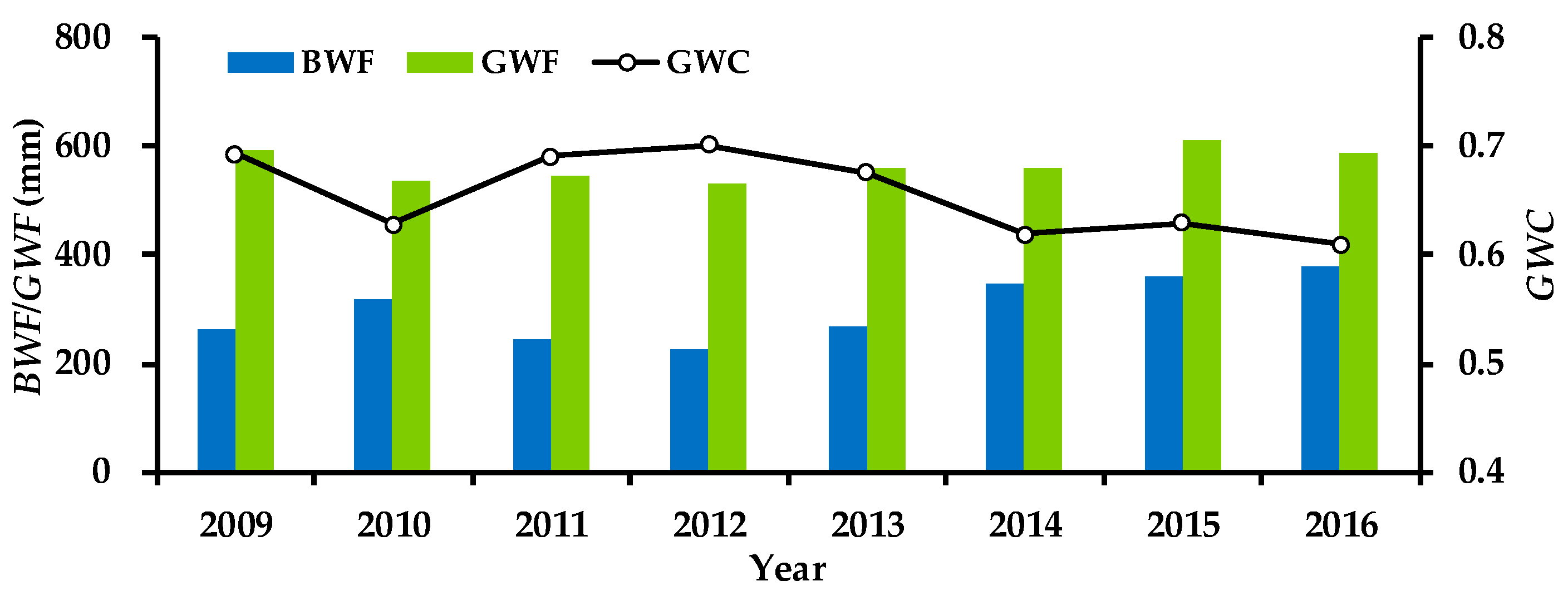
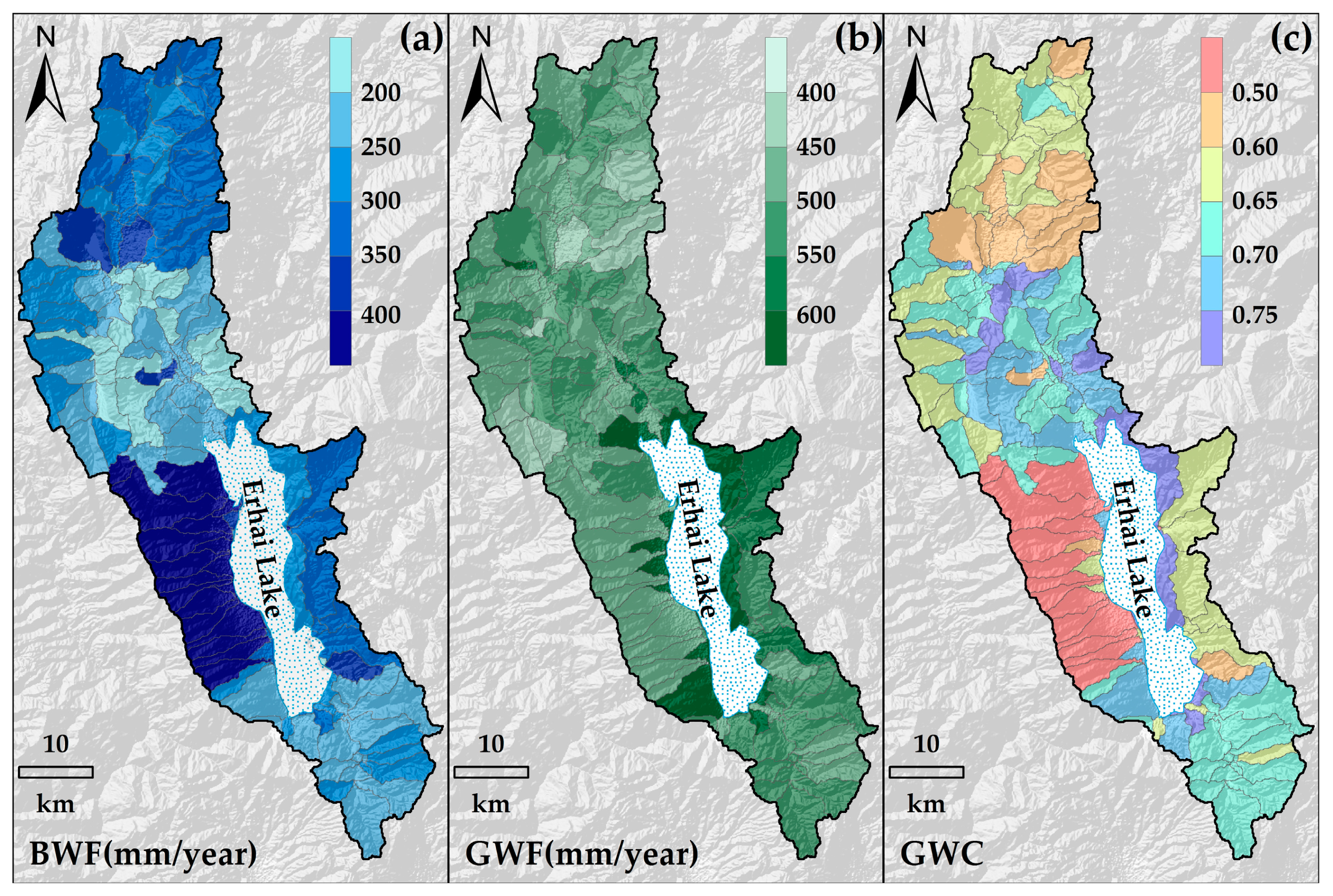
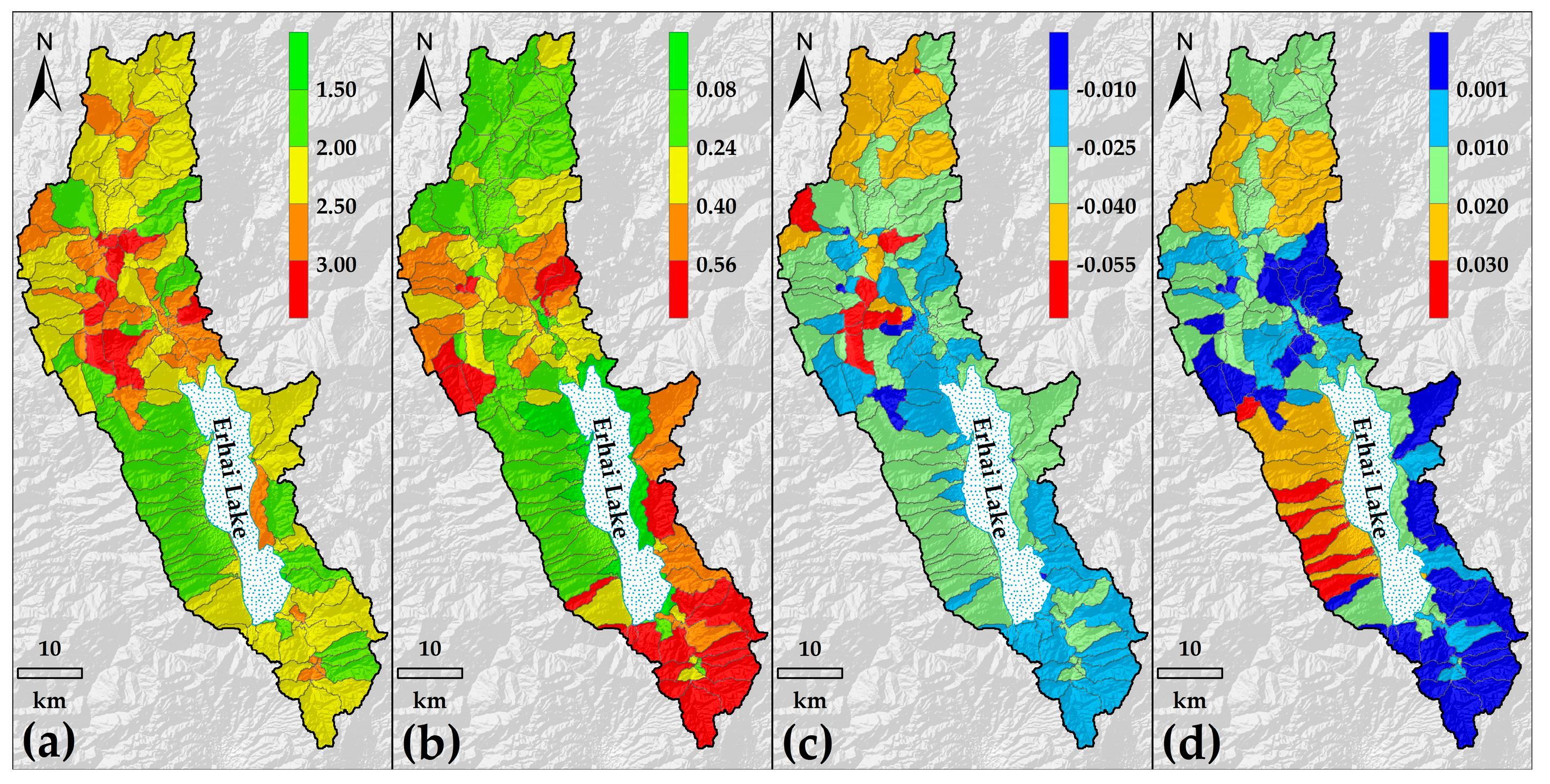
3.3. Spatial and Temporal Variability of Blue and Green Water Flows in the Erhai Lake Basin

The annual average of BWF and GWF during the period 2009 to 2016 across the ELB were 288.9 mm and 562.3 mm, respectively. The variation coefficients were 0.18 and 0.15 for BWF and GWF, respectively, which means that the change of GWF was relatively more stable than that of BWF. It is mainly because that the GWF is influenced by various factors (e.g., precipitation and temperature) while the precipitation is the major factor affecting the BWF [52,53,54,55]. In the ELB, the linear correlation coefficient between precipitation and BWF was high to 0.81. But the relationship between GWF and precipitation/temperature was more complicated.

Both the BWF and GWF increased at the entire basin level in the recent 8 years. As a result, the GWC decreased by 0.01 per year during the study period (Figure 8). The changes in precipitation and temperature in the ELB are illustrated in Figure 9. It could be found that the precipitation has been increasing since 2011 (Figure 9a) which is contrary to the change of temperature (Figure 9b and Figure 9c). In this wetter and colder condition, the runoff (blue water) has increased faster than the evapotranspiration (green water), leading to a lower GWC.

The spatial variation of annual average BWF, GWF, and GWC are illustrated in Figure 10. It is obvious that the spatial distribution of BWF was uneven. The BWF shows a higher value in the west of Erhai Lake, where is called Eighteen Streams Region, with a BWF of more than 400 mm/year. The other main area of water-yield is in the mountainous regions located in the north and east of Erhai Lake, with the BWF ranging from 300 to 400 mm/year (Figure 10a). Compared with BWF, the spatial distribution of GWF is more homogeneous. The GWF in most parts of the ELB changed with a range of 450 to 550 mm. The areas with a high-value of GWF were mainly distributed around Erhai Lake. In the low altitude region, especially in the north and east of the ELB, the GWF is a large percentage of the water flow (Figure 10b), generally the GWC was more than 0.7. The trend of the GWC is downward with altitude (Figure 10c). This is mainly due to higher precipitation at high altitude along with low temperatures and evapotranspiration rates. Consequently water-yield is abundant [56,57,58].

3.4. Sensitivity of Blue and Green Water Flows to Climate Change

With the parameterized SWAT model, the blue water flow and green water flow can be simulated in the hypothetical climatic scenarios. Then the sensitivity of these water flows to climate change can be estimated.

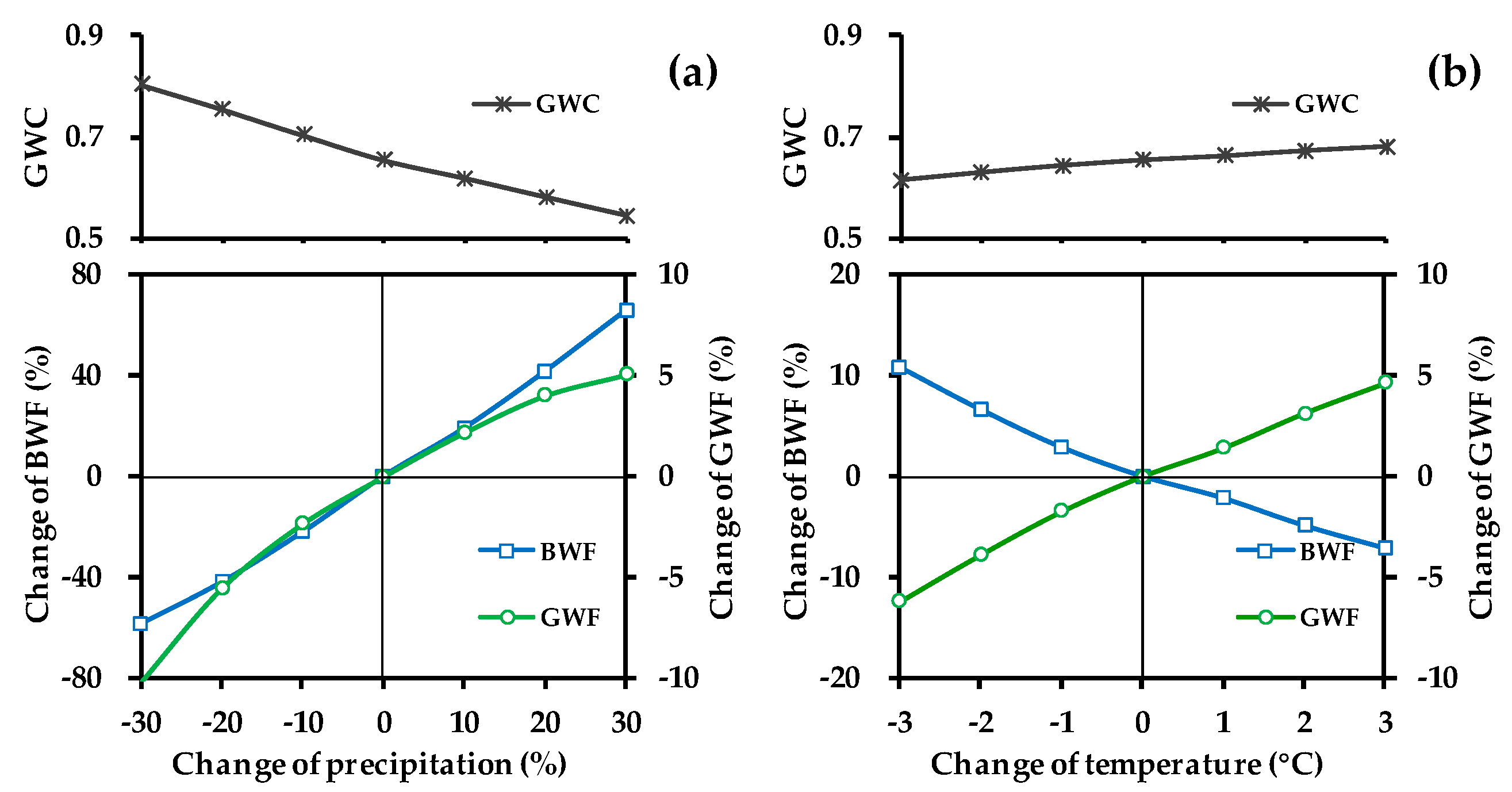
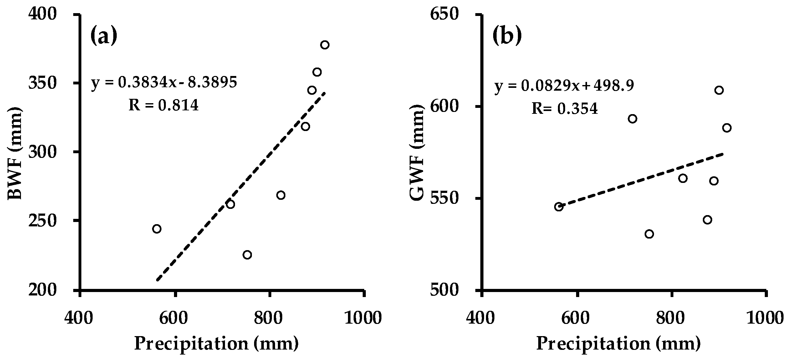
3.4.1. Sensitivity of Blue and Green Water Flows to Precipitation and Temperature at the Basin Scale

In the hydrographs for precipitation change (−30% to +30%) in Section 2.4, the BWF and GWF would increase with the precipitation. From Figure 11a, we can observe that a 10% increase in precipitation will result in a 20.8% increase in the BWF, but the GWF was less susceptible to precipitation change, showing an increase of 2.5% when precipitation increases by 10%. The GWC would decrease obviously as the precipitation increasing. It varied from 0.80 to 0.54 as precipitation amount changes with −30% and +30%, respectively.

The impact of temperature on the BWF was the opposite to the GWF under the temperature change scenarios (−3 °C to +3 °C). Figure 11b indicates that the BWF would decrease as the temperature increased, owing to a higher evapotranspiration rate in the warmer conditions. It was shown to decrease by 8.8 mm (nearly 3%) with a 1 °C reduction. But both the GWF and temperature would have a similar positive trend when temperature changes between −3.0 and 3.0 °C. The GWF would rise by 10.0 mm (about 1.7%) when temperature increases by 1.0 °C. In the hypothesis for temperature change, GWC would change slightly with an increase of approximately 0.01 for a corresponding 1.0 °C temperature increase.

3.4.2. Sensitivity of Blue and Green Water Flows to Precipitation and Temperature at the Sub-Basin Scale

With the sensitivity index of water flow to climate change defined in Section 2.4, the spatial difference of sensitivity can be illustrated as Figure 12. In the low altitude regions located on the north and south of Erhai Lake, the BWF was more sensitive to precipitation. These regions are characterized by a lower precipitation–runoff coefficient. Similar results can also be found in Jones et al. [59], Bao et al. [60], and Yuan et al. [61]. The sensitivity of GWF to precipitation has similar spatial distribution characteristics with BWF. The more sensitive areas were also predominately located in the north and south of the Erhai Lake. These spatial distribution characteristics can be scientifically explained according to the Budyko hypothesis [62]. Water availability and energy are major factors that control evapotranspiration (GWF). The lower altitude region usually has a warmer climate. Thus, the GWF was primarily limited by the precipitation and sensitivity to it in the north and south of Erhai Lake. The Budyko hypothesis also explains why the GWF in the mountainous area located on the north and west of the ELB was more sensitive to temperature than that in other sub-basins. The weather condition is usually colder in the mountainous area, and evapotranspiration mainly depends on the energy under the wet condition. Therefore, along with the rising air temperature, the GWF would increase obviously in the mountainous areas, especially in the Cangshan Mountain, where the precipitation is abundant. As a consequence, the BWF would decrease significantly in these regions.

4. Discussion

4.1. Comparison of the Sensitivity of Blue Water Flow and Green Water Flow

The sensitivity of BWF and GWF to precipitation and temperature has been analyzed in this study. However, other climatic factors, such as humidity, radiation, wind speed, have not been taken into consideration. From Figure 11 we can observe that the BWF was more sensitive to precipitation and temperature change compared with GWF. For example, an increase of 20% precipitation will result in an increase of 41.7% and 4.0% in BWF. The BWF was directly formed from precipitation, with correlation coefficient higher than 0.8 (Figure 13a). However, the relationship between precipitation and GWF was less obvious (Figure 13b). It is mainly because precipitation is not the only crucial factor for GWF. The air temperature, solar radiation, relative humidity, and wind speed are also important factors affecting GWF. Previous studies found that the decrease of GWF might be related to solar radiation or wind speed reduction [63,64,65], while the increase in wind speed or decrease in relative humidity might cause GWF increases [66,67,68]. Bao et al. have carried similar research in the Haihe River Basin of North China. Their research has also found that the GWF was less sensitivity to precipitation compared with BWF. Taking the Taolinkou catchment in the Haihe River Basin as an example, the BWF and GWF would decrease by 39% and 14% if precipitation decreased by 20% [60]. Besides, the response of BWF and GWF to precipitation and temperature is nonlinear. Thus, the sensitivity of water flows to climate change might be different in different climatic scenarios. But the sensitivity index designed in this study cannot be used to investigate this law. Another sensitivity index is needed to solve the above-mentioned problem in a future study.

4.2. Uncertainty Analysis

The major uncertainties in this study come from input data, model parameters, and model structure. To be specific, the gridded data (0.25° × 0.25°) provided by the CMADS was used in this study. Compared with the weather data (only Dali station) provided by National Meteorological Information Center, this dataset can describe the spatial difference of meteorological factors distribution. However, the area of ELB is less than 3000 km², and there are only 17 grid points in and around the ELB. Thus, the precipitation data from limited points could not really represent regional precipitation. Higher spatial resolution data might be useful for hydrological simulation in this small watershed. In addition, although there are several hydrologic stations in the study area, only Liancheng Station can provide daily discharge data and be used for parameter calibration, while other stations can only be used to measure water level. Thus, the differences between optimized parameters and real parameters of the ELB cannot be avoided. Therefore, this study will do further research on water flows simulation by SWAT model based on parameters transfer method in the ELB. The different parameters transfer methods, such as spatial proximity, physical similarity, and comprehensive similarity, should be compared. Furthermore, evapotranspiration is an important process for assessing water flows as well as precipitation. The BWF and GWF are associated with the methods used to estimate potential evapotranspiration (ET₀). The SWAT model provides three methods, namely, Penman–Monteith method [69,70], Priestley–Taylor method [71] and Hargreaves method [72] to calculate potential evapotranspiration. In this study, the Penman–Monteith method was selected. Obviously, if the other two methods were used for ET₀ estimation, the sensitivity of water flows to precipitation and temperature would be different from the results in this study. Quantitative uncertainties derived from the model structure in sensitivity analysis should be further analyzed by using different ET₀ estimation methods or even different hydrological models.

4.3. Method for Green Water Flow Estimation

In this study, the GWF was assessed by SWAT model, which is a water balance method. From Section 3.2, we can find that the SWAT model was a reliable representation of streamflow in the ELB according to the observed data. But we can only evaluate the GWF simulation indirectly at long time scales based on the water balance principle. However, the simulation of monthly actual evapotranspiration (ET_a) or GWF has not been verified in this study because of the lack of long-term actual observed data. It can be concluded that the quantitative analysis of BWF’s response to climate change has higher reliability than that of GWF.

Beyond water-balance derived ET_a, the GWF can also be estimated by remotely-sensed images. Based on the energy balance Bowen ratio method [73], the relationship between satellite-based vegetation indices and ET_a can be established, and then the GWF can be estimated indirectly [74]. The SWAT-based GWF and satellite-based GWF can be comparatively evaluated by each other. In addition, with the data assimilation methods, e.g., Ensemble Kalman Filter (EnKF) [75], the SWAT-based GWF and satellite-based GWF can also be assimilated. It might be an important work to improve the confidence of for the sensitivity of GWF to climate change and would be carried on in further study.

4.4. Impact of Land Use/Cover Change on Blue and Green Water Flow

Water availability are directly influenced by the climate variability. Since the land use/cover is relatively stable and climate variability affected the water flows more significantly than land use/cover change (LUCC) [76], this research did not analyze the impact of LUCC on blue and green water flow in the ELB. This does not mean that this kind of impact should be ignored. In fact, the components of water availability, such as surface runoff, inter flow, groundwater recharge, evapotranspiration, ect., principally depend on land use/cover [77]. Hence, a change in land use/cover of the ELB can alter the proportions of blue and green water flows. Analysis of multi-year land use data obtained from the RESDC dataset showed that the ELB has witnessed a remarkable expansion of built-up land and rapid shrinkage of agricultural land in the recent 35 years. From 1980 to 2014, the built-up land has significantly increased by 100.8%. The expansion area covered 67.5 km², accounting for 2.6% of the study area. In contrast, agricultural land has decreased by 10.7%. This reduced area was as large as 69.8 km², representing 2.7% of the ELB (

Table 2. Land use change from 1980 to 2015.

Land Use	Year 1980		Year 2015		Change
	Area (km2)	Percentage (%)	Area (km2)	Percentage (%)	Area (km2)	Percentage (%)
Agricultural land	651.8	25.5	582.0	22.8	−69.8	−10.7
Forest	838.8	32.9	851.5	33.4	12.8	1.5
Grassland	703.8	27.6	693.8	27.2	−10.0	−1.4
Water	265.9	10.4	261.0	10.2	−4.9	−1.8
Built-up land	67.0	2.6	134.5	5.3	67.5	100.8
Waste land	25.0	1.0	29.4	1.2	4.4	17.5

). Considering these actual situations of land use change, the urban expansion scenarios and ecological restoration scenarios can be further established in the following research. Then the impact of climate and land-use/cover change on water flows can be analyzed comprehensively. Furthermore, the land use/cover in the future (e.g., 2020 year or 2050 year) can be predicted by cellular automata (CA) model [78]. Then the change of blue and green water flows in the future period can be estimated, which would be useful for water resources planning.

5. Conclusions

Using the CMADS reanalysis data, SWAT model, and the hypothetical climatic scenarios, the impact of climate variability on blue and green water flow in Erhai Lake Basin was investigated. According to this research, the following conclusions have been made:

The CMADS performed well in terms of correlation with gauge observations from Dali station. The statistic results showed that the CMADs has a considerable skill in representing the PDFs of daily gauge observations: The skill score was 0.799, 0.964, and 0.957 for daily precipitation, Maximum temperature and Minimum temperature, respectively. At the monthly scale, the CMADS underestimated the precipitation with a bias of −6.6% while ir overestimated the Maximum temperature and Minimum temperature by 0.14 °C and 0.44 °C, respectively. Both precipitation and temperature were highly consistent with the monthly gauge observations. It can be concluded that the CMADS can capture the climate characteristics of the Erhai Lake Basin. In addition, the CMADS reanalysis data can be widely applied in hydrological simulation and water plan and management, especially in basins with no or few data. Moreover, the SWAT model has been proved to be applicable in simulating the hydrologic processes in the Erhai Lake Basin, with E_NS and R² values greater than 0.75 and RE value less than 5%.

Estimated by the SWAT model, the annual average of blue water flow and green water flow during 2009 to 2016 across the Erhai Lake Basin were 288.9 mm and 562.3 mm, respectively. Blue water flow has increased while green water flow has decreased in the recent 8 years, owing to increasing precipitation and decreasing temperature, leading to a lower GWC. The spatial distribution of blue water flow was uneven in Erhai Lake Basin. It was higher in the mountainous regions with higher precipitation–runoff coefficients, such as Eighteen Streams Region, with blue water flow more than 400 mm/year. However, the spatial distribution of green water flow is more homogeneously, changing with a range of 450 to 550 mm/year in most areas. The trend of the GWC goes downward with the increase of altitude. It is because precipitation is higher while temperatures and evapotranspiration rates are lower at high altitude.

Blue water flow was more sensitive to precipitation and temperature change compared with green water flow. A 10% increase in precipitation can bring about a 20.8% increase in blue water flow while only a 2.5% increase in green water flow at basin scale. When temperature increases by 1.0 °C, blue water flow and green water flow would change by −3% and 1.7%, respectively. Blue water flow and green water flow were more sensitive to precipitation in the low altitude regions located at the north and south of Erhai Lake, which is characterized by a lower precipitation–runoff coefficient and warmer condition. In contrast, blue water flow and green water flow were more sensitive to temperature in the mountainous area, which is characterized by colder and wetter condition.

This study provided insights into blue and green water flows response to climate variability in the Erhai Lake Basin, which will help policymakers and administrators manage water resources in the context of climate change. Spatial variations of sensibility of water flows to climate variability imply that specific adaptation measures in different regions should be taken in the Erhai Lake Basin.

References

1. Zhuang, X.; Li, Y.; Nie, S.; Fan, Y.; Huang, G. Analyzing climate change impacts on water resources under uncertainty using an integrated simulation—Optimization approach. J. Hydrol. 2018, 556, 523–538. [Google Scholar] [CrossRef]
2. Miara, A.; Macknick, J.E.; Vörösmarty, C.J.; Tidwell, V.C.; Newmark, R.; Fekete, B. Climate and water resource change impacts and adaptation potential for US power supply. Nat. Clim. Chang. 2017, 7, 793–798. [Google Scholar] [CrossRef]
3. Liang, W.; Bai, D.; Wang, F.; Fu, B.; Yan, J.; Wang, S.; Yang, Y.; Long, D.; Feng, M. Quantifying the impacts of climate change and ecological restoration on streamflow changes based on a Budyko hydrological model in China’s Loess Plateau. Water Resour. Res. 2015, 51, 6500–6519. [Google Scholar] [CrossRef]
4. Chen, Y.; Li, Z.; Fan, Y.; Wang, H.; Deng, H. Progress and prospects of climate change impacts on hydrology in the arid region of northwest China. Environ. Res. 2015, 139, 11–19. [Google Scholar] [CrossRef] [PubMed]
5. Mishra, V.; Kumar, R.; Shah, H.L.; Samaniego, L.; Eisner, S.; Yang, T. Multi-model assessment of sensitivity and uncertainty of evapotranspiration and a proxy for available water resources under climate change. Clim. Chang. 2017, 141, 451–465. [Google Scholar] [CrossRef]
6. Gohar, A.A.; Cashman, A. A methodology to assess the impact of climate variability and change on water resources, food security and economic welfare. Agric. Syst. 2016, 147, 51–64. [Google Scholar] [CrossRef]
7. Simonovic, S.P. Bringing future climatic change into water resources management practice today. Water Resour. Manag. 2017, 31, 2933–2950. [Google Scholar] [CrossRef]
8. Arnell, N.W. Climate change and global water resources. Glob. Environ. Chang. 1999, 9, 31–49. [Google Scholar] [CrossRef]
9. Huntington, T.G. Evidence for intensification of the global water cycle: Review and synthesis. J. Hydrol. 2006, 319, 83–95. [Google Scholar] [CrossRef]
10. Chen, G.; Zhao, W. Green water and its research progresses. Adv. Earth Sci. 2006, 21, 221–227. [Google Scholar]
11. Schuol, J.; Abbaspour, K.C.; Yang, H.; Srinivasan, R.; Zehnder, A.J.B. Modeling blue and green water availability in Africa. Water Resour. Res. 2008, 44, W07406. [Google Scholar] [CrossRef]
12. Vanham, D. A holistic water balance of Austria-how does the quantitative proportion of urban water requirements relate to other users? Water Sci. Technol. 2012, 66, 549–555. [Google Scholar] [CrossRef] [PubMed]
13. Liu, J.; Yang, H. Spatially explicit assessment of global consumptive water uses in cropland: Green and blue water. J. Hydrol. 2009, 384, 187–197. [Google Scholar] [CrossRef]
14. Zang, C.; Liu, J. Trend analysis for the flows of green and blue water in the Heihe River basin, northwestern China. J. Hydrol. 2013, 502, 27–36. [Google Scholar] [CrossRef]
15. Ding, W. A study on the characteristics of climate change around the Erhai area, China. Resour. Environ. Yangtze Basin 2016, 25, 599–605. (In Chinese) [Google Scholar]
16. Huang, H.; Wang, Y.; Li, Q. Climatic characteristics over Erhai Lake basin in the late 50 years and the impact on water resources of Erhai Lake. Meteorol. Mon. 2013, 39, 436–442. (In Chinese) [Google Scholar]
17. Li, W.; Yang, C.; Liu, E.; Peng, Z.; Liu, Q. Multiple time scale analysis of water resources in Erhai Lake Basin in recent 59 years. Chin. J. Agrometeorol. 2010, 31, 10–15. (In Chinese) [Google Scholar]
18. Li, Y.; Li, B.; Zhang, K.; Zhu, J.; Yang, Q. Study on spatiotemporal distribution characteristics of annual precipitation of Erhai Basin. J. China Inst. Water Resour. Hydropower Res. 2017, 15, 234–240. (In Chinese) [Google Scholar]
19. Arias, R.; RodríguezBlanco, M.L.; Taboadacastro, M.M.; Nunes, J.P.; Keizer, J.J.; Taboadacastro, M.T. Water resources response to changes in temperature, rainfall and CO2 concentration: A first approach in NW Spain. Water 2014, 6, 3049–3067. [Google Scholar] [CrossRef]
20. Falkenmark, M. Land-water linkages: A synopsis. Land and water integration and river basin management. FAO Land Water Bull. 1995, 1, 15–16. [Google Scholar]
21. Zhang, W.; Zha, X.; Li, J.; Liang, W.; Ma, Y.; Fan, D.; Li, S. Spatiotemporal change of blue water and green water resources in the headwater of Yellow River Basin, China. Water Resour. Manag. 2014, 28, 4715–4732. [Google Scholar] [CrossRef]
22. Chen, C.; Hagemann, S.; Liu, J. Assessment of impact of climate change on the blue and green water resources in large river basins in China. Environ. Earth Sci. 2015, 74, 6381–6394. [Google Scholar] [CrossRef]
23. Lee, M.H.; Bae, D.H. Climate change impact assessment on green and blue water over Asian monsoon region. Water Resour. Manag. 2015, 29, 2407–2427. [Google Scholar] [CrossRef]
24. Glavan, M.; Pintar, M.; Volk, M. Land use change in a 200-year period and its effect on blue and green water flow in two Slovenian Mediterranean catchments-lessons for the future. Hydrol. Process. 2013, 27, 3964–3980. [Google Scholar] [CrossRef]
25. Fazeli, F.I.; Farzaneh, M.R.; Besalatpour, A.A.; Salehi, M.H.; Faramarzi, M. Assessment of the impact of climate change on spatiotemporal variability of blue and green water resources under CMIP3 and CMIP5 models in a highly mountainous watershed. Theor. Appl. Climatol. 2018. [Google Scholar] [CrossRef]
26. Zhou, F.; Xu, Y.; Chen, Y.; Xu, C.; Gao, Y.; Du, J. Hydrological response to urbanization at different spatio-temporal scales simulated by coupling of CLUE-S and the SWAT model in the Yangtze River Delta region. J. Hydrol. 2013, 485, 113–125. [Google Scholar] [CrossRef]
27. Fan, M.; Shibata, H. Simulation of watershed hydrology and stream water quality under landuse and climate change scenarios in Teshio River watershed, northern Japan. Ecol. Indic. 2015, 50, 79–89. [Google Scholar] [CrossRef]
28. Villarini, G.; Krajewski, W.F.; Smith, J.A. New paradigm for statistical validation of satellite precipitation estimates: Application to a large sample of the TMPA 0.25 3-hourly estimates over Oklahoma. J. Geophys. Res. Atmos. 2009, 114. [Google Scholar] [CrossRef]
29. Nijssen, B.; Lettenmaier, D.P. Effect of precipitation sampling error on simulated hydrological fluxes and states: Anticipating the Global Precipitation Measurement satellites. J. Geophys. Res. Atmos. 2004, 109. [Google Scholar] [CrossRef] [Green Version]
30. Conti, F.L.; Hsu, K.L.; Noto, L.V.; Sorooshian, S. Evaluation and comparison of satellite precipitation estimates with reference to a local area in the Mediterranean Sea. Atmos. Res. 2014, 138, 189–204. [Google Scholar] [CrossRef]
31. Li, C.; Tang, G.; Hong, Y. Cross-evaluation of ground-based, multi-satellite and reanalysis precipitation products: Applicability of the Triple Collocation method across Mainland China. J. Hydrol. 2018, 562, 71–83. [Google Scholar] [CrossRef]
32. Meng, X.; Wang, H. Significance of the China meteorological assimilation driving datasets for the SWAT Model (CMADS) of East Asia. Water 2017, 9, 765. [Google Scholar] [CrossRef]
33. Meng, X.; Wang, H.; Shi, C.; Wu, Y.; Ji, X. Establishment and Evaluation of the China Meteorological Assimilation Driving Datasets for the SWAT Model (CMADS). Water 2018, 10, 1555. [Google Scholar] [CrossRef]
34. Meng, X.; Wang, H.; Cai, S.; Zhang, X.; Leng, G.; Lei, X.; Shi, C.; Liu, S.; Shang, Y. The China Meteorological Assimilation Driving Datasets for the SWAT Model (CMADS) Application in China: A Case Study in Heihe River Basin. Preprints 2016. [Google Scholar] [CrossRef]
35. Meng, X.; Wang, H.; Wu, Y.; Long, A.; Wang, J.; Shi, C.; Ji, X. Investigating spatiotemporal changes of the land-surface processes in Xinjiang using high-resolution CLM3.5 and CLDAS: Soil temperature. Sci. Rep. 2017, 7, 13286. [Google Scholar] [CrossRef] [PubMed] [Green Version]
36. Meng, X.; Dan, L.; Liu, Z. Energy balance-based SWAT model to simulate the mountain snowmelt and runoff—Taking the application in Juntanghu watershed (China) as an example. J. Mt. Sci. 2015, 12, 368–381. [Google Scholar] [CrossRef]
37. Meng, X.; Wang, H.; Lei, X.; Cai, S.; Wu, H. Hydrological Modeling in the Manas River Basin Using Soil and Water Assessment Tool Driven by CMADS. Tehnički Vjesnik 2017, 24, 525–534. [Google Scholar]
38. Wang, Y.; Meng, X. Snowmelt runoff analysis under generated climate change scenarios for the Juntanghu River basin in Xinjiang, China. Tecnol. Y Cienc. Agua 2016, 7, 41–54. [Google Scholar]
39. Meng, X. Simulation and spatiotemporal pattern of air temperature and precipitation in Eastern Central Asia using RegCM. Sci. Rep. 2018, 8, 3639. [Google Scholar] [CrossRef] [PubMed] [Green Version]
40. Meng, X. Spring Flood Forecasting Based on the WRF-TSRM mode. Tehnički Vjesnik 2018, 25, 27–37. [Google Scholar]
41. Vu, T.; Li, L.; Jun, K. Evaluation of MultiSatellite Precipitation Products for Streamflow Simulations: A Case Study for the Han River Basin in the Korean Peninsula, East Asia. Water 2018, 10, 642. [Google Scholar] [CrossRef]
42. Gao, X.; Zhu, Q.; Yang, Z.; Wang, H. Evaluation and hydrological application of CMADS against TRMM 3B42V7, PERSIANN-CDR, NCEP-CFSR, and gauge-based datasets in Xiang River Basin of China. Water 2018, 10, 1225. [Google Scholar] [CrossRef]
43. Zhou, S.; Wang, Y.; Chang, J.; Guo, A.; Li, Z. Investigating the dynamic influence of hydrological model parameters on runoff simulation using sequential uncertainty fitting-2-based multilevel-factorial-analysis method. Water 2018, 10, 1177. [Google Scholar] [CrossRef]
44. Tian, Y.; Zhang, K.; Xu, Y.-P.; Gao, X.; Wang, J. Evaluation of potential evapotranspiration based on CMADS reanalysis dataset over China. Water 2018, 10, 1126. [Google Scholar] [CrossRef]
45. Hu, Y.; Peng, J.; Liu, Y.; Tian, L. Integrating ecosystem services trade-offs with paddy land-to-dry land decisions: A scenario approach in Erhai Lake basin, southwest China. Sci. Total Environ. 2018, 625, 849–860. [Google Scholar] [CrossRef] [PubMed]
46. Crook, D.; Elvin, M.; Jones, R.; Ji, S.; Foster, G.; Dearing, J. The History of Irrigation and Water Control in China’s Erhai Catchment: Mitigation and Adaptation to Environmental Change. In Mountains: Sources of Water, Sources of Knowledge; Springer: Berlin, Germany, 2008. [Google Scholar]
47. Nash, J.E.; Sutcliffe, J.V. River flow forecasting through conceptual models part I-A discussion of principles. J. Hydrol. 1970, 10, 282–290. [Google Scholar] [CrossRef]
48. Gupta, H.; Sorooshian, S.; Yapo, P. Status of automatic calibration for hydrologic models: Comparison with multilevel expert calibration. J. Hydrol. Eng. 1999, 4, 135–143. [Google Scholar] [CrossRef]
49. Kumar, S.; Merwade, V. Impact of watershed subdivision and soil data resolution on SWAT model calibration and parameter uncertainty. J. Am. Water Resour. Assoc. 2009, 45, 1179–1196. [Google Scholar] [CrossRef]
50. Yin, J.; Yuan, Z.; Yan, D.; Yang, Z.; Wang, Y. Addressing climate change impacts on streamflow in the Jinsha River Basin based on CMIP5 Climate Models. Water 2018, 10, 910. [Google Scholar] [CrossRef]
51. Jiang, S.; Ren, L.; Yong, B.; Yuan, F.; Gong, L.; Yang, X. Hydrological evaluation of the TRMM multi-satellite precipitation estimates over the Mishui basin. Adv. Water Sci. 2014, 25, 641–649. (In Chinese) [Google Scholar]
52. Zheng, H.; Zhang, L.; Zhu, R.; Liu, C.; Sato, Y.; Fukushima, Y. Responses of streamflow to climate and land surface change in the headwaters of the Yellow River Basin. Water Resour. Res. 2009, 45, W00A19. [Google Scholar] [CrossRef]
53. Lan, Y.; Zhao, G.; Zhang, Y.; Wen, J.; Hu, X.; Liu, J.; Gu, M.; Chang, J.; Ma, J. Response of runoff in the headwater region of the Yellow River to climate change and its sensitivity analysis. J. Geogr. Sci. 2010, 20, 848–860. [Google Scholar] [CrossRef]
54. Liu, Q.; Mcvicar, T.R. Assessing climate change induced modification of penman potential evaporation and runoff sensitivity in a large water-limited basin. J. Hydrol. 2012, 464, 352–362. [Google Scholar] [CrossRef]
55. Xu, C.; Singh, V. Evaluation of three complementary relationship evapotranspiration models by water balance approach to estimate actual regional evapotranspiration in different climatic regions. J. Hydrol. 2005, 308, 105–121. [Google Scholar] [CrossRef]
56. Wang, C.; Zhou, X. Effect of the recent climate change on water resource in Heihe river basin. J. Arid Land Resour. Environ. 2010, 24, 60–65. (In Chinese) [Google Scholar]
57. Guo, Q.; Yang, Y.; Chen, X.; Chen, Z. Annual Variation of Heihe River Runoff during 1957–2008. Prog. Geogr. 2011, 30, 550–556. (In Chinese) [Google Scholar]
58. Zang, C.; Liu, J.; Velde, M.; Kraxner, F. Assessment of spatial and temporal patterns of green and blue water flows under natural conditions in inland river basins in Northwest China. Hydrol. Earth Syst. Sci. 2012, 16, 2859–2870. [Google Scholar] [CrossRef] [Green Version]
59. Jones, R.N.; Chiew, F.H.S.; Boughton, W.C.; Zhang, L. Estimating the sensitivity of mean annual runoff to climate change using selected hydrological models. Adv. Water Resour. 2006, 29, 1419–1429. [Google Scholar] [CrossRef] [Green Version]
60. Bao, Z.; Zhang, J.; Liu, J.; Wang, G.; Yan, X.; Wang, X.; Zhang, L. Sensitivity of hydrological variables to climate change in the Haihe river basin, China. Hydrol. Process. 2012, 26, 2294–2306. [Google Scholar] [CrossRef]
61. Yuan, Z.; Yan, D.; Yang, Z.; Yin, J.; Zhang, C.; Yuan, Y. Projection of surface water resources in the context of climate change in typical regions of China. Hydrol. Sci. J. 2017, 62, 283–293. [Google Scholar] [CrossRef]
62. Budyko, M.I. Climatic factors of the external physical-geographical processes. Gl Geofiz Obs. 1950, 19, 25–40. (In Russian) [Google Scholar]
63. Brutsaert, W.; Parlange, M.B. Hydrologic cycle explains the evaporation paradox. Nature 1998, 396, 30. [Google Scholar] [CrossRef]
64. Golubev, V.S.; Lawrimore, J.H.; Groisman, P.Y.; Speranskaya, N.A.; Zhuravin, S.A.; Menne, M.J.; Peterson, T.C.; Thomas, C.; Malone, R.W. Evaporation changes over the contiguous united states and the former USSR: A reassessment. Geophys. Res. Lett. 2001, 28, 2665–2668. [Google Scholar] [CrossRef]
65. Xu, C.; Gong, L.; Jiang, T.; Chen, D.; Singh, V.P. Analysis of spatial distribution and temporal trend of reference evapotranspiration and pan evaporation in Changjiang (Yangtze river) catchment. J. Hydrol. 2006, 327, 81–93. [Google Scholar] [CrossRef]
66. Yu, P.; Yang, T.; Chou, C. Effects of climate change on evapotranspiration from paddy fields in southern Taiwan. Clim. Chang. 2002, 54, 165–179. [Google Scholar] [CrossRef]
67. Burn, D.H.; Hesch, N.M. Trends in evaporation for the Canadian prairies. J. Hydrol. 2007, 336, 61–73. [Google Scholar] [CrossRef]
68. Dinpashoh, Y.; Jhajharia, D.; Fakheri-Fard, A.; Singh, V.P.; Kahya, E. Trends in reference crop evapotranspiration over Iran. J. Hydrol. 2011, 399, 422–433. [Google Scholar] [CrossRef]
69. Monteith, J.L. Evaporation and environment. In Proceedings of the 19th Symposium of the Society for Experimental Biology, New York, NY, USA, 1 January 1965; Cambridge University Press: Cambridge, UK, 1965; pp. 205–233. [Google Scholar]
70. Allen, R.G.; Jensen, M.E.; Wright, J.L.; Burman, R.D. Operational estimates of reference evapotranspiration. Agron. J. 1989, 81, 650–662. [Google Scholar] [CrossRef]
71. Priestley, C.H.B.; Taylor, R.J. On the assessment of surface heat flux and evaporation using large-scale parameters. Mon. Weather Rev. 1972, 100, 81–92. [Google Scholar] [CrossRef]
72. Hargreaves, G.L.; Hargreaves, G.H.; Riley, J.P. Agricultural benefits for Senegal River Basin. J. Irrig. Drain. Eng. 1985, 111, 113–124. [Google Scholar] [CrossRef]
73. Allen, R.G.; Pereira, L.S.; Howell, T.A.; Jensen, M.E. Evapotranspiration information reporting: I. Factors governing measurement accuracy. Agric. Water Manag. 2011, 98, 899–920. [Google Scholar] [CrossRef]
74. Nagler, P.L.; Glenn, E.P.; Kim, H.; Emmerich, W.; Scott, R.L.; Huxman, T.E.; Huete, A.R. Relationship between evapotranspiration and precipitation pulses in a semiarid rangeland estimated by moisture flux towers and MODIS vegetation indices. J. Arid. Environ. 2007, 70, 443–462. [Google Scholar] [CrossRef]
75. Sun, L.; Seidou, O.; Nistor, I.; Liu, K. Review of the Kalman type hydrological data assimilation. Hydrol. Sci. J. 2016, 61, 2348–2366. [Google Scholar] [CrossRef]
76. Zhao, A.; Zhu, X.; Liu, X.; Pan, Y.; Zuo, D. Impacts of land use change and climate variability on green and blue water resources in the Weihe river basin of northwest china. Catena 2016, 137, 318–327. [Google Scholar] [CrossRef]
77. Sajikumar, N.; Remya, R.S. Impact of land cover and land use change on runoff characteristics. J. Environ. Manag. 2015, 161, 460–468. [Google Scholar] [CrossRef] [PubMed]
78. Deng, Z.; Zhang, X.; Li, D.; Pan, G. Simulation of land use/land cover change and its effects on the hydrological characteristics of the upper reaches of the Hanjiang Basin. Environ. Earth Sci. 2015, 73, 1119–1132. [Google Scholar] [CrossRef]
Figure 1. Location of the Erhai Lake Basin (ELB), Southwest China.
Water 11 00424 g001
Figure 2. Schematic diagram of simulated components in the soil and water assessment tool (SWAT) model.
Water 11 00424 g002
Figure 3. The land use map (a), soil type map (b) and China Meteorological Assimilation Driving Datasets (CMADS) grid points in the ELB (c).
Water 11 00424 g003
Figure 4. Diagrams of CMADS- probability density functions (PDF) vs Gauge-PDF illustrating the total skill score.
Water 11 00424 g004
Figure 5. PDFs for the daily CMADS reanalysis data and gauge observations: (a) Precipitation; (b) Maximum temperature; (c) Minimum temperature.
Water 11 00424 g005
Figure 6. Scatter plots of the monthly CMADS reanalysis data and gauge observations: (a) Precipitation; (b) Maximum temperature; (c) Minimum temperature.
Water 11 00424 g006
Figure 7. Simulated and observed monthly streamflow at Liancheng station during the calibration period 2009 to 2014 and the validation period 2015 to 2016.
Water 11 00424 g007
Figure 8. Changes in water flows and green water coefficient from 2009 to 2016: The blue bar represents blue water flow (BWF), and the green bar represents green water flow (GWF). The line with circles represents the green water coefficient (GWC).
Water 11 00424 g008
Figure 9. Changes in annual precipitation (a), average Maximum temperature (b) and average Minimum temperature (c) from 2009 to 2016.
Water 11 00424 g009
Figure 10. The spatial distribution of annual average BWF (a) GWF (b), and GWC (c) (2009 to 2016).
Water 11 00424 g010
Figure 11. Sensitivity on BWF, GWF, and GWC impacted by precipitation change (a) and temperature change (b) in the ELB.
Water 11 00424 g011
Figure 12. Sensitivity on BWF and GWF impacted by precipitation or temperature change in the sub-basin scale. (a) Sensitivity of BWF to precipitation; (b) Sensitivity of GWF to precipitation; (c) Sensitivity of BWF to temperature; (d) Sensitivity of GWF to temperature.
Water 11 00424 g012
Figure 13. The relationship between precipitation and water flow in the ELB during 2009 to 2016: (a) precipitation vs. BWF; (b) precipitation vs. GWF.
Water 11 00424 g013