1. Introduction
Lentic freshwaters are acknowledged to play a crucial role in regulating the global ecosystem functions e.g., carbon cycle [
1] and they are among the Earth’s most threatened habitats in terms of intensity of anthropogenic pressures, biodiversity loss, and non-indigenous species introduction [
2,
3,
4].
They include an extreme variety of habitats differing in ecological characteristics and fragility [
5,
6]. Surface area represents one of the most apparent differentiating properties: indeed, lentic environments (304 million water bodies; 4.2 million km
2 in total area [
7]) include the lake Superior (82,000 km
2), together with small ponds, i.e., waterbodies less than 0.05 km
2 in area [
8].
Ponds and small lakes (hereafter PSL) have significant ecological functions [
9,
10]: among others, they provide a considerable contribution to inland water CO
2 and CH
4 emissions [
11]. In addition, they are, to date, recognized as important biodiversity hotspots, especially in mountainous regions, supporting a high species richness and contributing a high degree of rare species to regional pools ([
12,
13,
14,
15]; see also [
16] for an example on planktonic Calanoida). Noticeably, PSL are threatened by a number of anthropogenic pressures, including nutrient loading, contamination, acid rain, and invasion of exotic species [
17]. In addition, infilling (both natural and caused by direct habitat destruction), land drainage, decline in many of their traditional uses, and changes of function determine at a regional scale the drastic reduction in PSL number and connectivity [
12].
In the last decade, several investigations have focused on the diversity of benthic invertebrates, as they are excellent bio-indicators of PSL ecological integrity [
18,
19]. Local factors that are related with e.g., hydroperiod, environmental harshness, water chemistry, spatial connectivity, habitat heterogeneity, and presence of predators, have been recognized to influence the biodiversity of macroinvertebrate assemblages ([
20] and literature cited). At a regional scale, attention has been primarily given to the influence of waterbodies area [
21,
22,
23], while assuming, within the general theoretical background provided by the species-area relationship (SAR) hypothesis [
24], that basins’ size correlates with the number of microhabitats within the basin itself and with populations’ abundance, and thence inversely correlated with the likelihood of random extinctions. However, resolving the contribution to biodiversity patterns of environmental factors acting at a regional scale is, to date, essential to the implementation of effective conservation strategies in the face of e.g. deforestation and climate change ([
25,
26] and literature cited). Accordingly, several attempts have been made to model biodiversity of freshwater environments by means of regional bioclimatic factors [
27,
28].
In the present study, we focused on the diversity of crustacean zooplankton assemblages in 40 ponds and small lakes differing remarkably in terms of origin, extension, and altitude from a relatively wide region comprising part of Albania and North Macedonia. A recent faunal inventory focusing on ponds and lakes in the area [
29] provided the starting reference information on the taxonomic characteristics of the assemblages.
A number of studies have generally indicated a positive relationship between the surface area of lacustrine environments and zooplankton diversity (e.g., [
30,
31,
32]; but see [
13]); accordingly, crustacean zooplankton has been shown to have higher species richness in small ponds as compared with lakes [
16,
33,
34]. This notwithstanding, we hypothesized that area alone may not be an adequate predictor, and that local bioclimatic conditions may ultimately contribute in explaining diversity variations across waterbodies by influencing their physical-chemical characteristics, as observed in recent investigations on freshwater macroinvertebrates and macrophytes [
27,
28,
35]. This could be particularly true for waterbodies in mountainous habitats, where temperature and precipitation regimes intensely reflect the chemical-physical characteristics and hydroperiod of the waterbodies themselves [
36], regulating the harshness and stability of the aquatic environments and, in turn, the diversity of the biota living in them ([
22] and literature cited).
To verify the hypothesis and test whether bioclimatic factors can predict assemblages’ diversity, we identified a minimum adequate model (MAM) predicting assemblages’ diversity across the different waterbodies by means of a heuristic multiple regression approach and Bayesian Information Criterion model selection method while using satellite-derived bioclimatic variables as predictors. Multiple indices are, to date, available to quantify different aspects of biodiversity [
37]. Here, we identified predictive MAMs estimating the diversity of crustacean zooplankton assemblages in terms of species richness and average taxonomic distinctness.
Species richness is the most classical measure of biodiversity across ecosystems that has been extensively used in studies on lentic habitats (see references cited above). This index provides an incomplete understanding of biological variability, because it neglects information on the identity and taxonomic relationship among species, and it is hampered by a number of critical limitations [
38,
39]. Accordingly, we used the average taxonomic distinctness Δ+ [
40] to compare the taxonomic relatedness of species in the crustacean assemblages of every water body. In addition, we tested the influence of bioclimatic factors on crustacean assemblages in terms of species composition. To this end, multivariate approaches that are based on a canonical analysis of principal coordinates were used to model the changes in the structure of the assemblages as affected by bioclimatic variables, and identify relationships between the latter and specific groups of zooplankton taxa.
3. Results
3.1. General Features
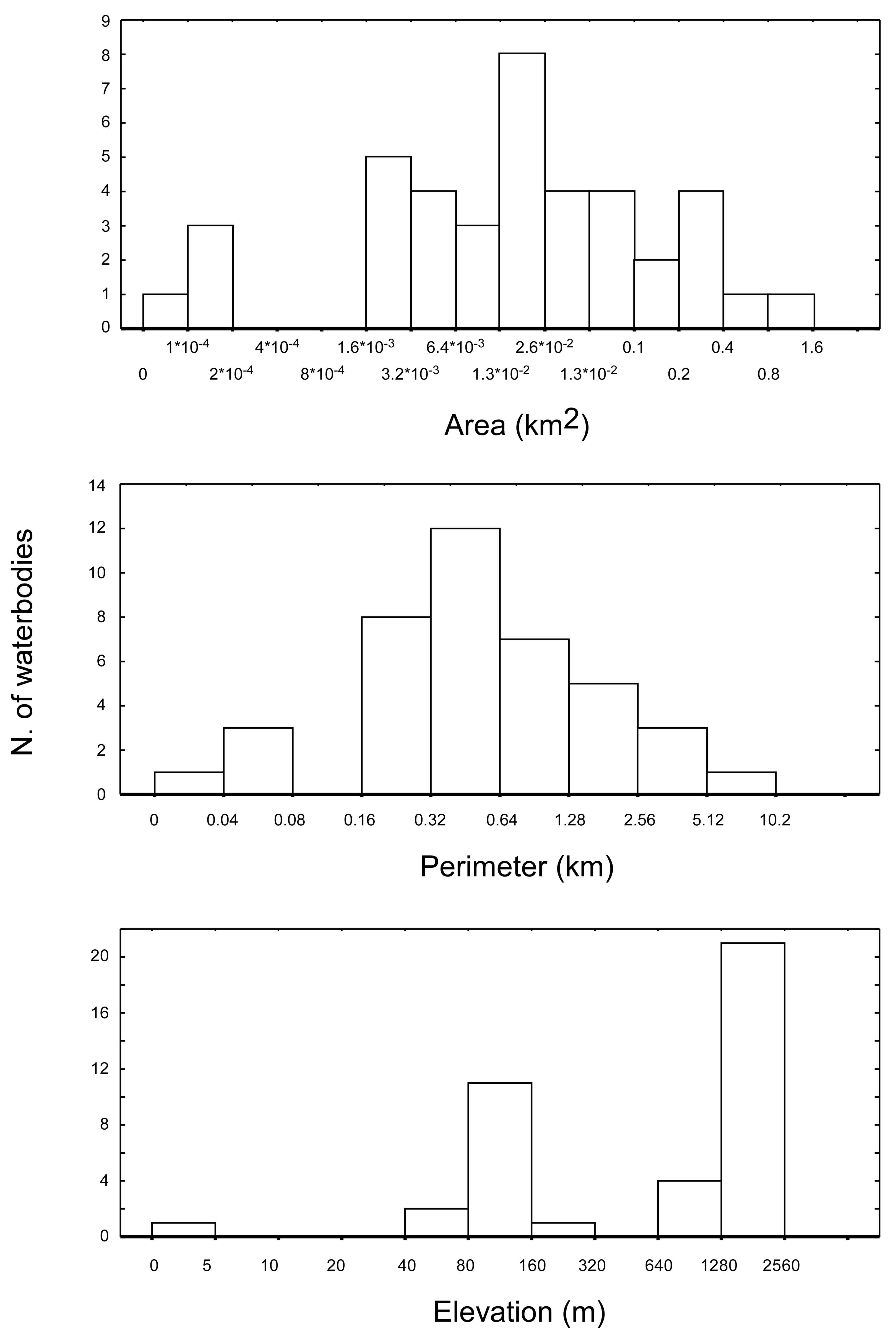
The 40 water bodies analysed, varied remarkably in terms of altitude, area, and perimeter (
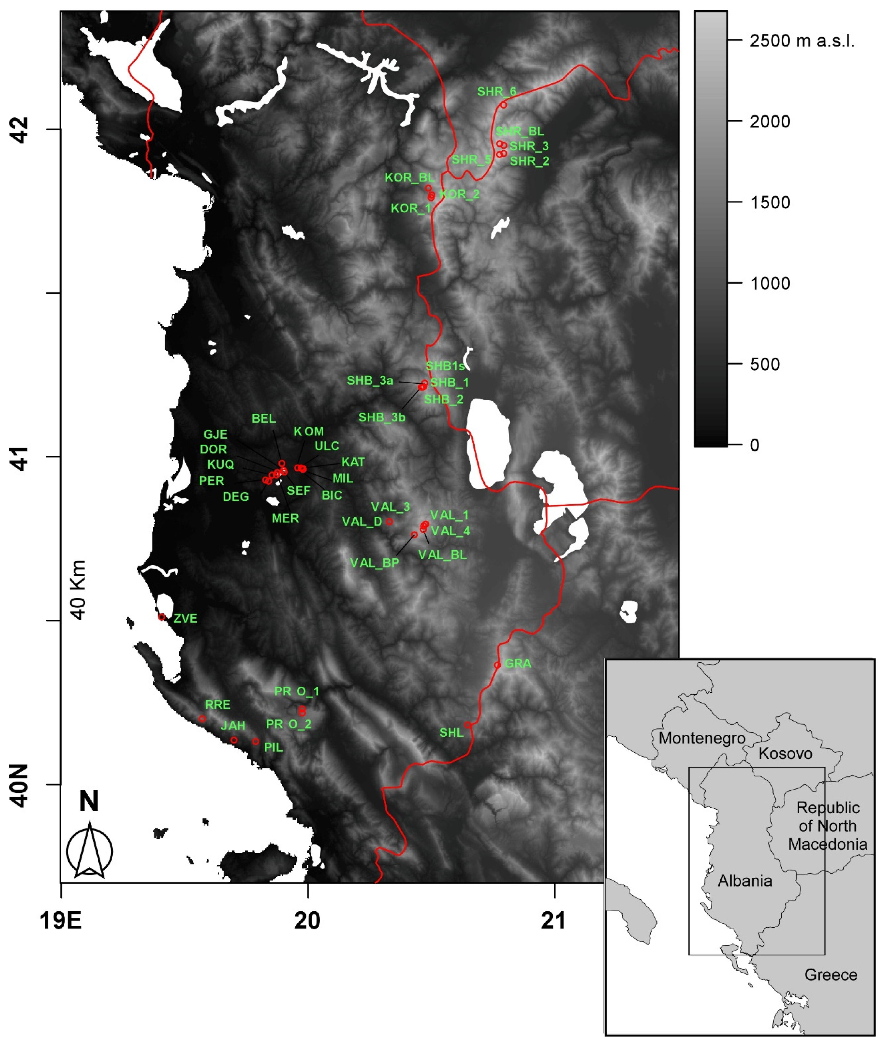
Figure 2). They showed an average altitude of 1168.3 m a.s.l. (± 141.9 m SE), ranging from 2 m a.s.l. (Narte Zvernec pond, ZVE in
Figure 1) to 2,435 m a.s.l. (SHR 5). The average surface extension was 0.09 km
2 ± 0.03 SE, ranging from 9.1×10
−4 to 0.86 km
2. The average perimeter was 1.01 ± 0.21 km, ranging between 0.035 and 6.1 km. For both of the variables, the minimum and maximum values corresponded with a small artificial pond in the karst highlands of Progonat (PRO1) and the Lake Seferan in the Dumre region (SEF).
In the 40 water bodies, 79 Crustacea species were identified in total, being almost equally distributed between the classes Branchiopoda and Hexanauplia (41 and 38 species respectively).
Among Branchiopoda, Anomopoda outnumbered the other two orders Ctenopoda and Haplopoda (38 vs. 2 and 1 species). Daphnia, Ceriodaphnia, and Moina were the genera that were characterized by the highest number of species (nine Daphnia species, four Moina species, and three Ceriodaphnia species) together representing the majority of all the sampled Anomopoda species. Ctenopoda were represented by the congeneric Diaphanosoma brachyurum and D. lacustris while Haplopoda by the single species Leptodora kindtii. The class Hexanauplia (alias Copepoda) was dominated by species belonging to the order Cyclopoida (31) and to a minor extent Calanoida (7). The genus Cyclops (seven species) together with Acanthocyclops, Paracyclops (four species each), and Mesocyclops (three species) constituted to the majority of the species in the order; Calanoida were represented by the genera Eudiaptomus (three species), Mixodiaptomus (two species each), and by Arctodiaptomus salinus and Neodiaptomus schmackeri.
The species showing the widest distributions were the Anomopoda
Bosmina longirostris (16 sites),
Chydorus sphaericus (15 sites), and
Daphnia longispina (14 sites) (
Table 2); in addition, the Cyclopoida
Mesocyclops leuckarti, the Calanoida
Mixodiaptomus tatricus, and the Ctenopoda
Diaphanosoma brachyurum occurred in 12 sampled sites.
As regarding high level taxa, only Anomopoda (Cladocera) were present in every site. Cyclopoida (Hexanauplia) were present in 38 sites (95% of the total), Calanoida (Hexanauplia) in 30 sites (75%), Ctenopoda (Cladocera) in four sites (10%), and Haplopoda (Cladocera) in three sites (7.5%).
3.2. Diversity Patterns and Bioclimatic Correlates
On average, 6.7 ± 0.4 species per water body were found, ranging between three (JAH, PIL, RRE) and 14 species (KOR 1). The taxonomic distinctness Δ+ of the different planktonic assemblages was on average 72.1 ± 0.78, ranging between 60 (SHB 2) and 88.9 (GRA).
The factor “origin” was the only exerting significant effects of the species richness of waterbodies (
Table 2), with the six artificial water bodies being included in the study characterized by lower S values as compared with natural basins (3.5 ± 0.22 vs. 7.29 ± 0.38, respectively). Conversely, negligible effects were generally observed for the taxonomic distinctness Δ+ (
Table 2).
The 25 predictor variables (
Table A1) were reduced to a set of nine characterized by negligible collinearity (
Table A2). They included five climatic variables (i.e., Isothermality, Temperature Seasonality, Mean Temperature of Wettest Quarter, Annual Precipitation, and Precipitation of Coldest Quarter), % tree and % non-tree vegetation cover, habitat heterogeneity, and water body surface. Besides water body surface, the variable Mean Temperature of Wettest Quarter showed the greatest among-water bodies variability (
Table A2), ranging from a minimum of −5.32 °C (SHB 2) to a maximum of 11 °C (ZVE). It was followed by % tree cover (varying between 1 and 70%, BEL and DEG, respectively) and % non-tree cover (ranging between 20 and approx. 81%, BEL-DEG and SHR 2, respectively).
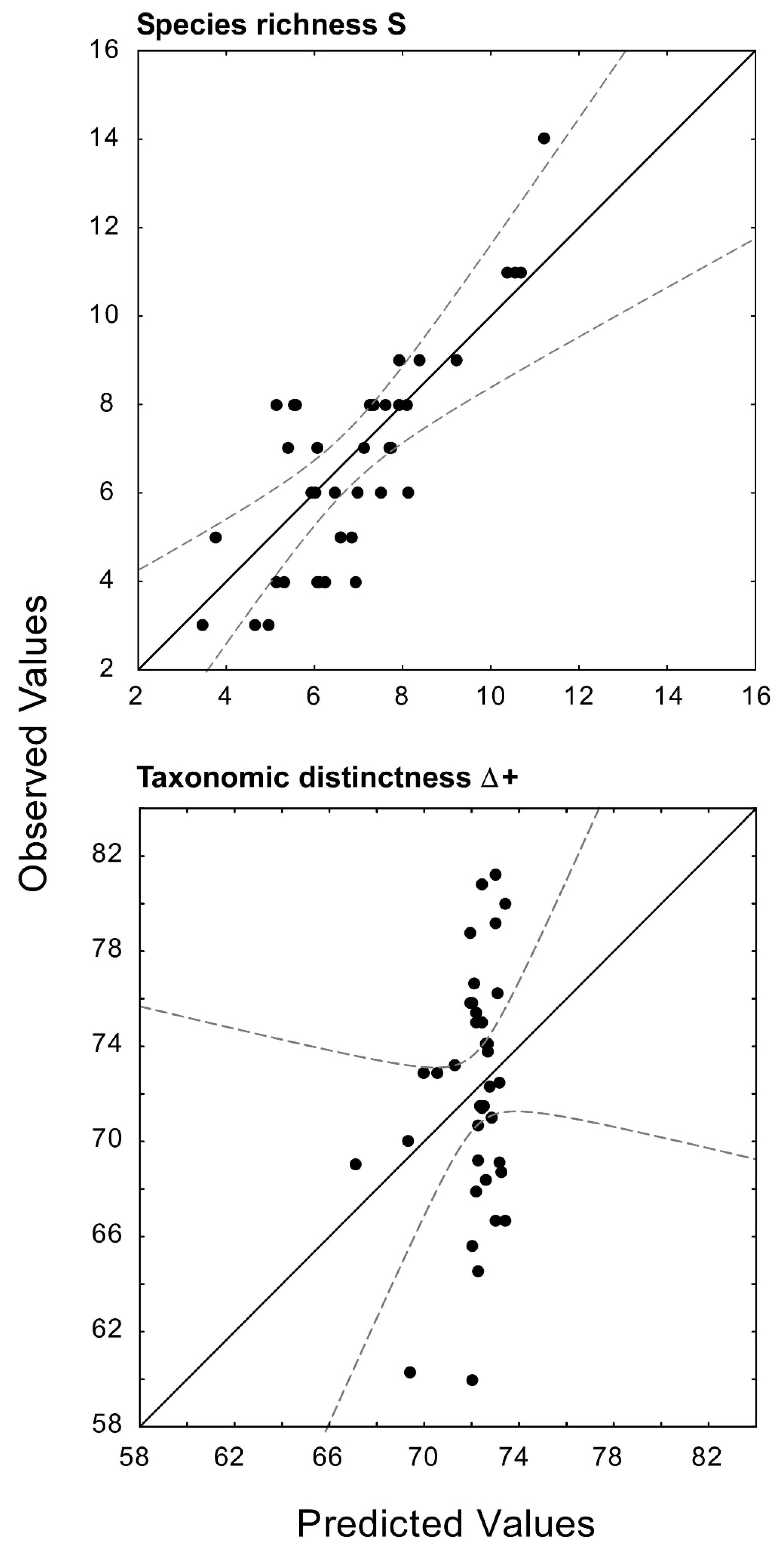
The heuristic search procedure identified a Minimum Adequate Model (MAM) predicting the variation of species richness S across the different water bodies relying on the three explanatory variables % non tree cover, Temperature Seasonality, and Mean Temperature of Wettest Quarter (
Figure 3; multiple
r = 0.58,
P = 0.002, d.f. = 3, 36). The MAM was characterized by the lowest
AICc value, and by an Akaike weight
wi approximately eight times larger than the second-best candidate, based on the variables Temperature Seasonality, Mean Temperature of Wettest Quarter, and Habitat heterogeneity (
Table 3). All of the predictors provided significant contributions to S variation across water bodies (minimum absolute
t value = 2.34,
P = 0.02 for the variable Mean Temperature of Wettest Quarter); the contributions of both % non-tree cover and Temperature Seasonality were positive (b = 0.27 ± 0.12 and 0.64 ± 0.15, respectively), while the Mean Temperature of the Wettest Quarter provided a negative contribution (b = −0.26 ± 0.14). Noticeably, none of the first ten best-performing models included water body area (
Table 3).
In contrast with species richness, the heuristic search procedure was unable to identify a MAM with a significant predictive power for taxonomic distinctness. The single variable % tree cover, resulted the best predictor of Δ+ (
Table 3); however, the correlation resulted in being non-significant (
r = 0.25,
P = 0.11, d.f. 1,38; see also
Figure 3). Other models showed an even worst performance, independently from the number of variables involved (
Table 3), indicating, in turn, that the taxonomic distinctness of the crustacean assemblages cannot be predicted by bioclimatic, landscape-scale factors.
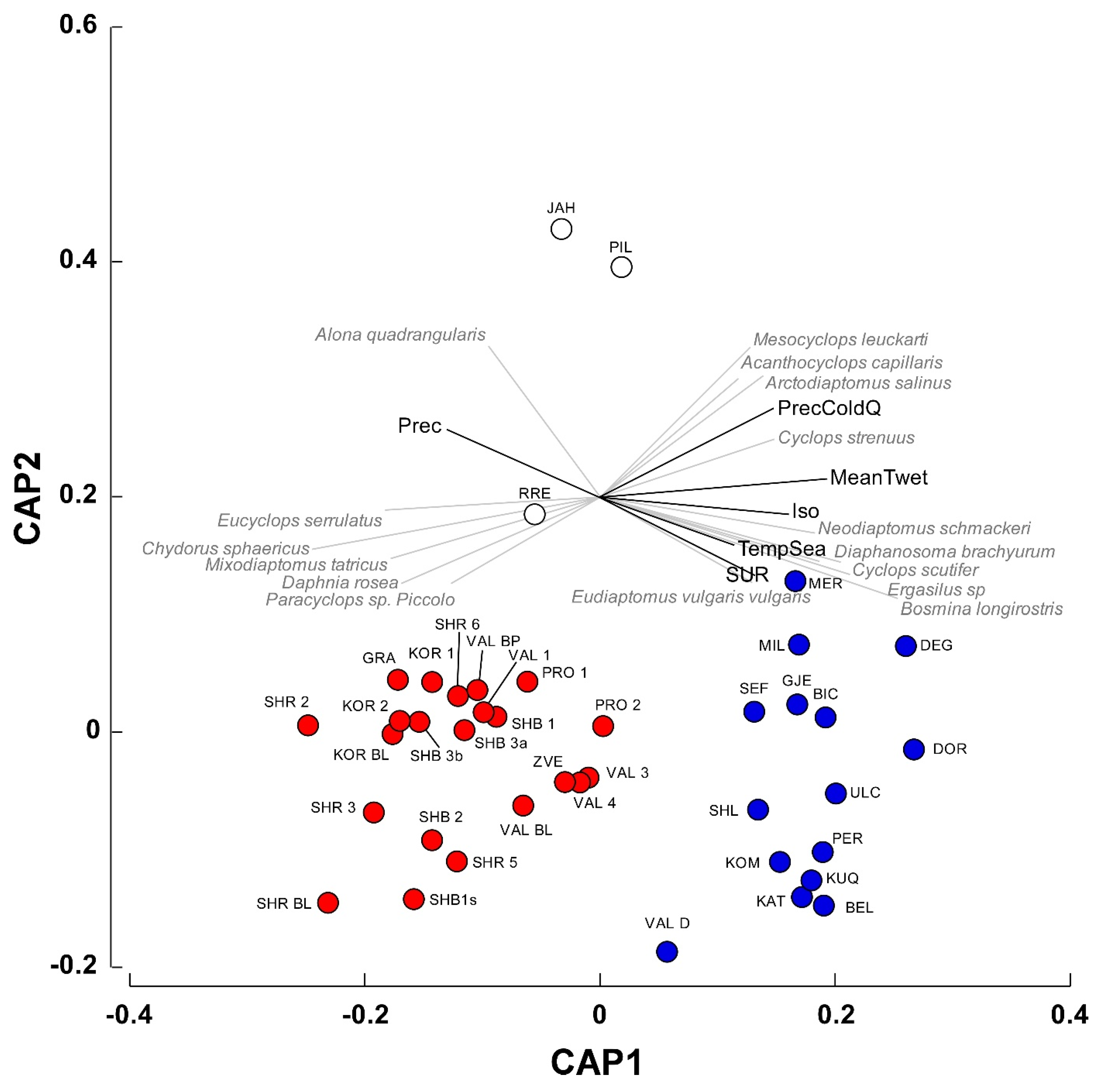
Canonical analysis of principal coordinates (CAP), followed by a confirmatory PERMANOVA test identified two main groups of waterbodies significantly different in terms of species composition (
Figure 4; Pseudo–F = 7.2, P(perm) = 0.001). The variables Isothermality, Mean Temperature of Wettest Quarter, Annual Precipitation, and Precipitation of Coldest Quarter showed a correlation (
r > 0.65) with the canonical axis 1 (
Figure 4) and significantly differed between the two groups of waterbodies (PERMANOVA, Pseudo–F = 27.4, P(perm) = 0.001). A Simper procedure indicated that the variable Mean Temperature of Wettest Quarter contributed by 32.2% to inter-group differences, followed by Isothermality and Annual Precipitation (28.6 and 24.2%, respectively).
In group1, the Mean Temperature of Wettest Quarter was remarkably lower than that determined for group2 (0.06 ± 0.69 vs. 8.44 ± 0.09 °C; t-test for separate variances: t = 9.41, P < 0.0001, 25.53 d.f.). Similarly, Isothermality showed lower values in group1 (33.91 ± 0.23 vs. 38.42 ± 0.24, t = 9.19, P < 0.0001, 29.52 d.f.), while the Annual Precipitation showed an inverse pattern (1098 ± 10.42 vs. 1012 ± 1.71 mm, t = −6.43, P < 0.001, 26.09 d.f.).
The analysis of the relationships between species occurrences and the canonical axis 1 (see
Table A2 for Spearman correlations for the complete list of species) indicated that
Eucyclops serrulatus,
Chydorus sphaericus,
Mixodiaptomus tatricus, and
Daphnia rosea in the first group were correlated mainly with Precipitation. The occurrences of
Neodiaptomus schmackeri,
Diapahnosoma brachyurum,
Cyclops scutifer,
Ergasilus sp,
Bosmina longirostris, and, to a lesser extent,
Mesocyclops leuckarti in the group2 were related with the variables Isothermality, Mean Temperature of Wettest Quarter, and Precipitation of Coldest Quarter.
4. Discussion
The earth is undergoing an accelerated rate of native ecosystem conversion and degradation and there is increased interest in measuring and modelling biodiversity while using landscape-scale, remotely-sensed predictors. Here, we made an attempt towards this direction while using crustacean zooplankton. This group of organisms, ubiquitous in lentic habitats, has been recently subjected to renewed interest as an effective bio-indicator of the environmental status of ponds and small lakes [
62,
63,
64,
65]. The heuristic procedure was used here to identify minimum adequate models predicting the diversity the crustacean zooplankton assemblages across the 40 waterbodies under analysis provided non-univocal results. On one hand, they showed that a subset of bioclimatic variables could effectively predict the variation in species richness and composition across the different waterbodies. On the other hand, they also indicated that the assemblages’ taxonomic distinctness Δ+ is unrelated with landscape-scale environmental drivers.
Before discussing these results, it must be considered that the emphasis we put on landscape and bioclimatic drivers of zooplankton diversity by no means imply that other chemical, physical, and biotic characteristics of the waterbodies, such as nutrient concentration, pH, depth, predators, aquatic vegetation, etc. are to be considered of secondary importance. A number of studies have unequivocally indicated that they can directly affect zooplankton species richness ([
66,
67] and references cited in the introduction; but see also further in this section). In addition, lake age [
68,
69], connectivity, and, in general, the spatial arrangement of the habitat have been acknowledged to play an important structuring role (e.g., [
70]; see also [
71] for a marine example). However, in the present study, a hierarchy of effects at different spatial and environmental scales is implicitly assumed, with landscape and bioclimatic drivers indirectly affecting the characteristics of the biota (including crustacean zooplankton) by affecting the chemical and physical conditions of the waterbodies. Indeed, the limited extension of the basins that were included in our study (
Figure 1) actually implies for them a low thermal inertia, and thus the ability to rapidly respond to the external climatic conditions [
72]. An indirect support to this view is also provided by the negligible predictive power of waterbodies’ area for assemblages’ S, Δ+, and species composition, confirming the results of investigations performed on the benthic fauna of high-altitude ponds [
22].
The best MAM included as predictors the degree of non-arboreal vegetation cover of the land areas neighboring the waterbodies, temperature seasonality, and mean temperature of the wettest quarter. The positive influence of the non-arboreal vegetation cover on species richness is consistent with the results of studies that were focused on macrobenthos in lotic habitats (e.g., [
73] and literature cited). This could be ascribed to a positive, indirect effect of lateral trophic enrichment on aquatic primary producers, increasing zooplankton diversity by a phytoplankton-mediated bottom up effect or, alternatively, promoting habitat heterogeneity through an increase in aquatic vegetation [
66,
74,
75].
Noticeably, the two temperature variables had contrasting effects on species richness: the lowest number of species was predicted to occur in waterbodies that were subjected to minimum temperature variability during the year and to maximum temperatures during the wettest months, i.e., in winter. The positive influence of temperature variability on patterns of species diversity has been acknowledged for zooplankton and other freshwater invertebrates [
76,
77], and can generally be ascribed to an effect of habitats environmental heterogeneity on empty niches availability, and, in turn, on species richness [
78]. The negative influence of the mean temperature of the wettest quarter (MeanTwet) on species richness can be explained while considering that the former scales negatively with the altitude of the water bodies (
r = −0.95,
P < 0.001, 38 d.f.). Thus, MeanTwet maximum values were observed for basins that were located at low altitudes, generally in highly anthropized areas. Accordingly, the lower species richness characterizing these environments might be actually determined by the interplay of a spectrum of anthropogenic perturbations, such as pollution, water caption, or introduction of predatory fish. Indeed, until 1990, the vast majority of low-altitudes waterbodies in Albania have been stocked with both native and non-indigenous fish species [
79], and fish predation has been repeatedly recognized to influence the species richness of zooplankton in lentic habitats [
80,
81].
The “assemble first, predict later” modelling strategy that was used in the present study was successful in predicting species richness and is generally acknowledged to have several advantages, among others an enhanced capacity to synthesize complex data into a form more readily interpretable by scientists and decision-makers [
82]. However, it is apparent that it presents important limitations, as testified by the failure in modeling taxonomic distinctness. Δ+ resulted in being not predictable, confirming the results of several investigations that have found weak or negligible relationships of the taxonomic distinctness of macrobenthic communities with environmental factors [
27,
83,
84]. Species richness S and taxonomic distinctness Δ+ are not conceptually (or mechanistically) related, and they behave differently [
44]. The lack of congruence between S and Δ+ and the negligible predictability of the latter is because S is likely to respond to short-term environmental changes in the waterbodies under analysis, while Δ+ is a proxy for phylogenetic diversity, reflecting a complex set of intrinsic and extrinsic traits and expressing evolutionary long-term adaptations to local environmental conditions [
85]. The canonical analysis of principal coordinates allowed for us to partially overcome these limitations, applying an “assemble and predict together” strategy [
82] in order to model changes in the species composition of planktonic assemblages and provide an advanced resolution of species-specific relationships with bioclimatic factors. The CAP analysis (
Figure 4) distinguished two distinct group of waterbodies, showing different climatic characteristics in terms of isothermality, mean temperature of the wettest quarter, and annual precipitation. The first (red circles in
Figure 4) was mainly constituted by high-altitude ponds and lakes (elevation 1725.3 ± 123.7 m, mean ± 1SE) distributed throughout the study area characterized by Crustacea species (e.g.,
Eucyclops serrulatus,
Mixodiaptomus tatricus) that are peculiar of pristine alpine environments [
86]. The second group (blue circles in
Figure 4) comprised low-altitude karst waterbodies that were located in the Dumre area (
Figure 1; elevation 239.9 ± 86.2 m, mean ± 1SE), where they are subjected to several anthropogenic pressures, including agricultural and urban pollution, eutrophication, and the introduction of non-indigenous fish species [
87]. Accordingly, the group is characterized by the occurrence of
Neodiaptomus schmackeri, an Australasian species of Chinese origin that was recently introduced in Albanian lentic habitats through fish stocking [
88] and the copepod
Ergasilus sp., whose adult females are ectoparasites of fish [
89].
Regarding the three isolated waterbodies in
Figure 4 (i.e., JAH, PIL, and RRE), they are artificial reservoirs located at 1330, 701, and 280 m a.s.l., respectively, being heavily affected by cattle frequentation (Belmonte, personal observation). Their isolation in the CAP diagram is due to the low species richness (three species in all the waterbodies), that might be ascribed to cattle-induced eutrophication conditions [
90]. However, it is worth noting that copepods vary their body size (at the community level and even for single species) inversely with the eutrophication level [
91,
92]. Thus, by using a plankton net with a mesh size of 200 μm, we may have underestimated the smaller component of the planktonic assemblages thus biasing the species count.
A final consideration deserves a brief mention. In this study, the spatial resolution of the bioclimatic layers (approximately 0.64 km
2) was lower than the area characterizing most of the ponds and lakes included in the analysis (
Figure 2). In other words, the bioclimate spatial grid “matched” the dimensions of the waterbodies, the latter being completely included (and described in terms of climate and vegetation cover) within the same grid cell. Additional studies including a wider size range of waterbodies as well as bioclimatic layers resolved at different spatial resolutions are necessary to provide a more complete picture of the actual relationships linking bioclimatic factors and the diversity of lentic zooplankton at multiple regional and environmental scales.


