3.1. Analysis of the Wave Data
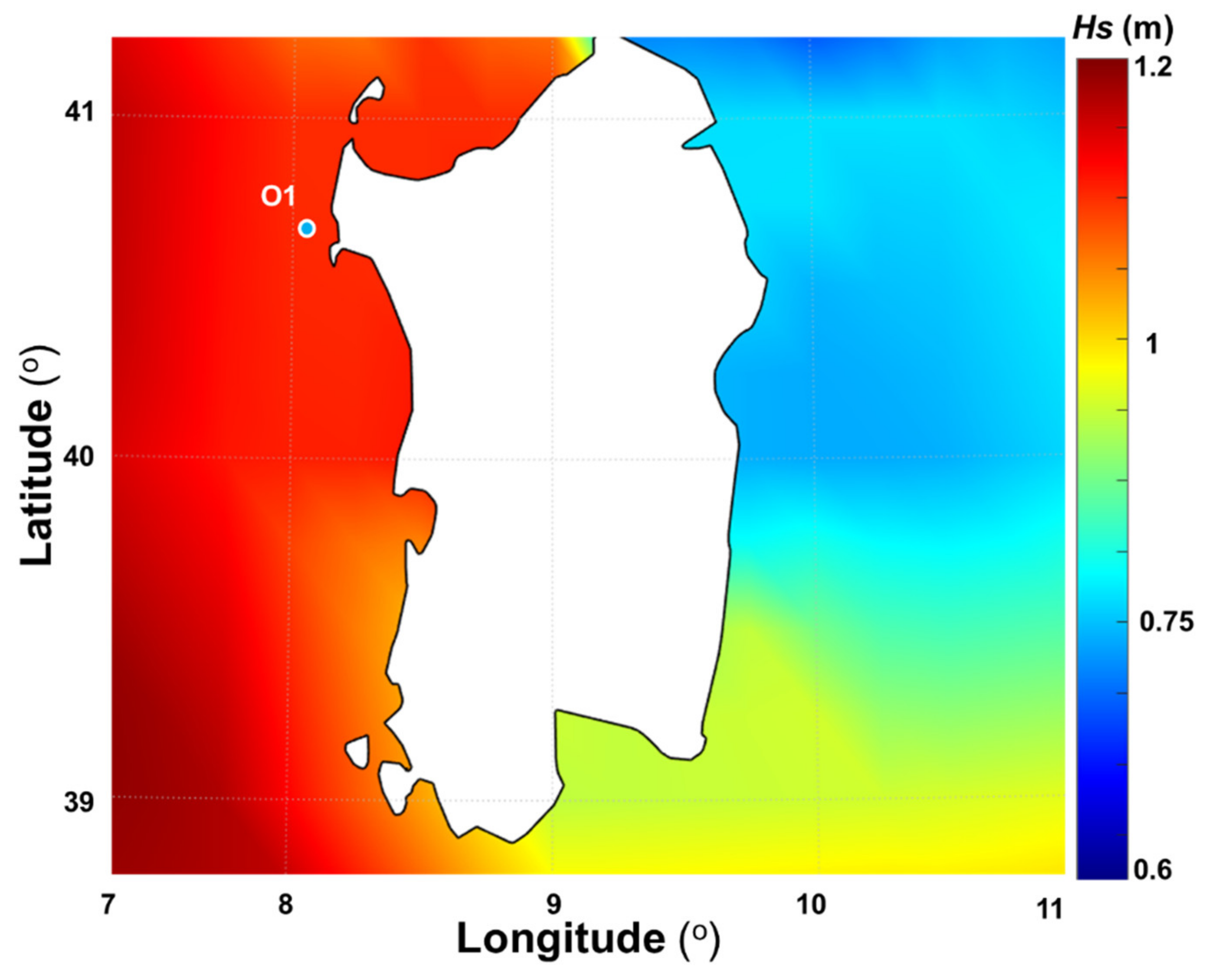
Figure 3 presents the average
Hs spatial distribution (average values) resulting from processing the ERA-interim data. The site O1 that was further used to identify the conditions occurring on the external boundary of the SWAN computational domain was also included. According to these data, it is clear that the western part of Sardinia presented higher wave conditions, with a maximum
Hs average value of 1.2 m compared to values of 0.75 m that were characteristic of the eastern part. According to these results, a wave farm implemented near the Porto Ferro area may represent a win–win project, since it is expected to generate some electricity production, on one hand, and to reduce the erosion effects associated with wave action, on the other hand.
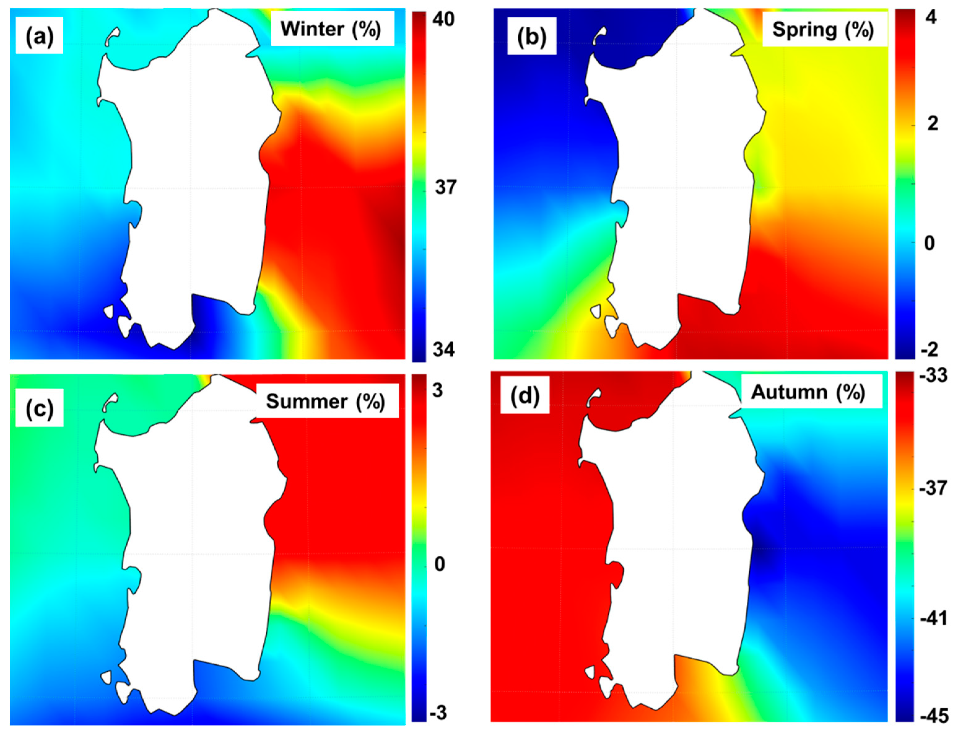
As a next step, the seasonal variations (in %) are presented in
Figure 4, being defined for: a) winter (December, January, February); b) spring (March, April, May); c) summer (June, July, August); and d) autumn (September, October, November). These seasonal variations were computed as the
Hs differences (in %) between the average values corresponding to the four main seasons and the average values corresponding to the total distribution divided by the same average values corresponding to the total distribution, considering the 40-years of ERA-interim data. This figure gives a picture of how the significant wave height was biased in each season in relation to the
Hs mean value for the total time.
Reporting on the total distribution, we noticed during winter an increase of the significant wave height with almost 40% for the eastern sector, while in the south–west a minimum of 34% was observed. The Porto Ferro conditions were between these two values. A mixed pattern occurred during spring, when in the north–west a decrease of almost 2% was noticed, compared to an increase of 4% in the southeast. In the central part of Sardinia, there were some areas presenting little or no fluctuations. During summer, more significant variations were noticed in the eastern side, whereas in the northeast an Hs increase of 3% occurred, while in the southern extremity a decrease was observed. Autumn seemed to be the least suitable season for the wave energy production, when decreases of the Hs values in the range of 33%–45% were noticed.
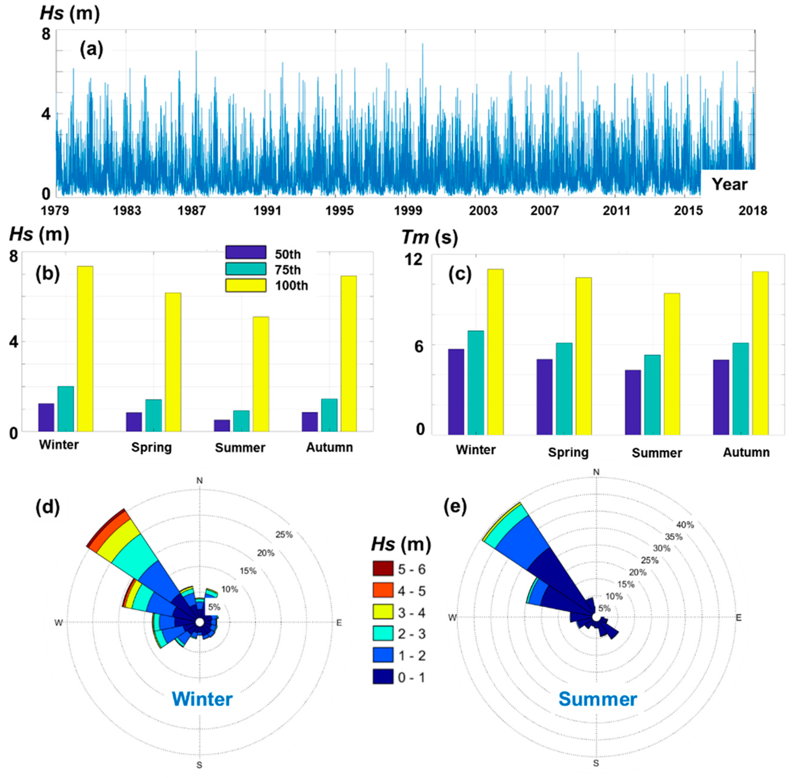
Figure 5 presents the wave conditions for the reference point O1. From the analysis of the time series, we noticed that the
Hs values could often reach values of 6 m. In terms of percentile analysis (
Figure 5b),
Hs indicated close values during winter and autumn. Thus, a maximum value of 7.35 m was noticed. For the other two seasons (spring and summer), the Hs values were in the range of 0.84–6.17 m (spring) and 0.52–5.1 m (summer). As for the wave period, an extreme value of 11 s was expected in the winter, followed by 10.9 s in autumn, and 9.4 s in summer. A minimum wave period value of 4.3 s was expected in summer, and this value could increase up to 5.7 s in winter. From the analysis of the wave directions (
Figure 5d,e), we noticed that there were no significant differences in terms of directions, both distributions (winter and summer) indicating the northwest sector (315°) as dominant. On the other hand, important differences occurred in terms of the
Hs classes, the winter distribution indicating values higher than four meters.
Table 2 summarizes the main statistical values presented in
Figure 5. As a next step, only two scenarios were considered for the SWAN simulations. These were summer (A and B) and winter (A and B).
3.2. Coastal Impact of the Generic Farm(s)
There are various approaches considering the degree of absorption of the wave energy by a marine energy farm. This depends on the wave energy converters (WECs) considered and also on the characteristics of the incoming waves. The most important wave parameters related to the wave energy absorption are the significant wave height, wave period, and wave direction. Thus, this is a dynamic process, and the most relevant indicator related to the wave energy absorption is the capture that can be estimated with certain accuracy for each particular situation. However, in the present work a generic marine farm is considered together with some relevant scenarios defined from the analysis of the long term wave parameters in the geographical space targeted. That is why an average absorption coefficient of 25% was considered in the present work. Several authors consider this value a realistic approach for a generic wave farm, as in the case of Rusu and Onea at 20% [
4] or Onea and Rusu at 25% [
42]. In the work of Stokes and Conley [
43], a WEC derived absorption index was proposed that could go up to 42%.
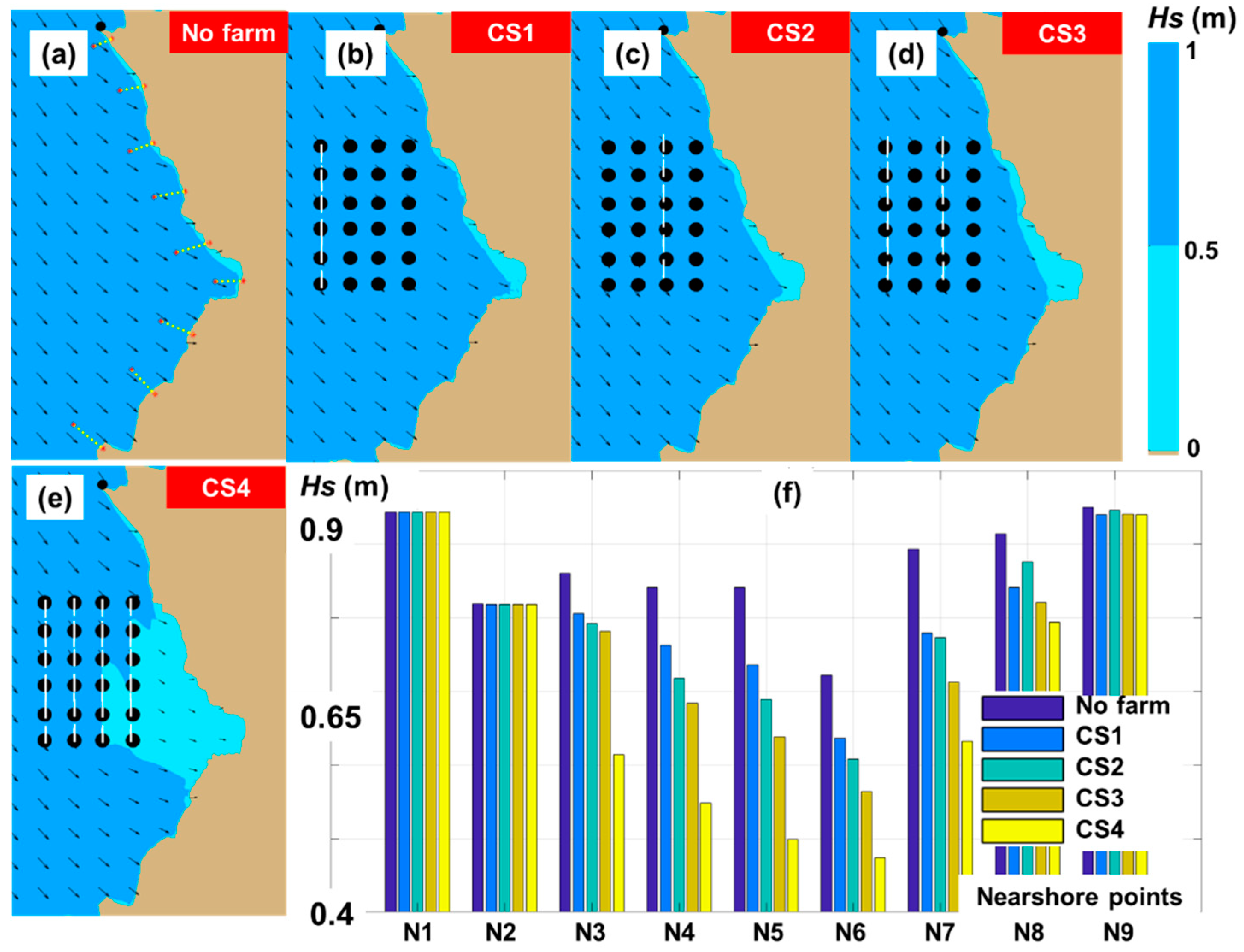
From this perspective, a first evaluation is provided in
Figure 6 for the scenario Summer A. From the spatial distribution of the wave fields (subplots 6a–e), we noticed that the impact of the generic farm was less visible for the scenario CS1 compared to CS4, where in the area between the marine farm and the coastline we noticed lower values. A more accurate evaluation was provided by the analysis performed in the N-points. Thus, in the case of the points N1, N2, and N9 no variation in the presence of the generic farm occurred. Looking at the shadowing effects, we noticed that for the scenario that involved a particular wave direction (NW) and the orientation of the WEC lines in the geographical space, little (or no) variations were expected for these sites. Therefore, these points were used as a reference in order to assess the accuracy of the results, and no variation was expected regardless of the wave conditions or scenario considered.
By comparing the scenarios CS1 and CS2, we noticed that the impact of the wave farm was more visible for the scenario CS2, except the point N8, when a reverse pattern was noticed. In general, there were relatively small differences between the scenarios CS1, CS2 and CS3, while a significant impact is noticed for CS4, especially in the case of the reference points N3–N7.
Table 3 presents the
Hs differences (in %) between the no farm scenario and the four scenarios considered. In the case of the points N1, N2 and N9 the variation is negligible, being expected a maximum attenuation of 1.1%. The sites N4 and N5 indicate in general higher values that start from 14% and reach a maximum of 46% in the case of CS4. Compared to the two line configuration (CS3), the scenario involving four generic marine farms (CS4) seems to offer a more effective coastal protection that can reduce at half the significant wave heights in some cases (ex: point N4).
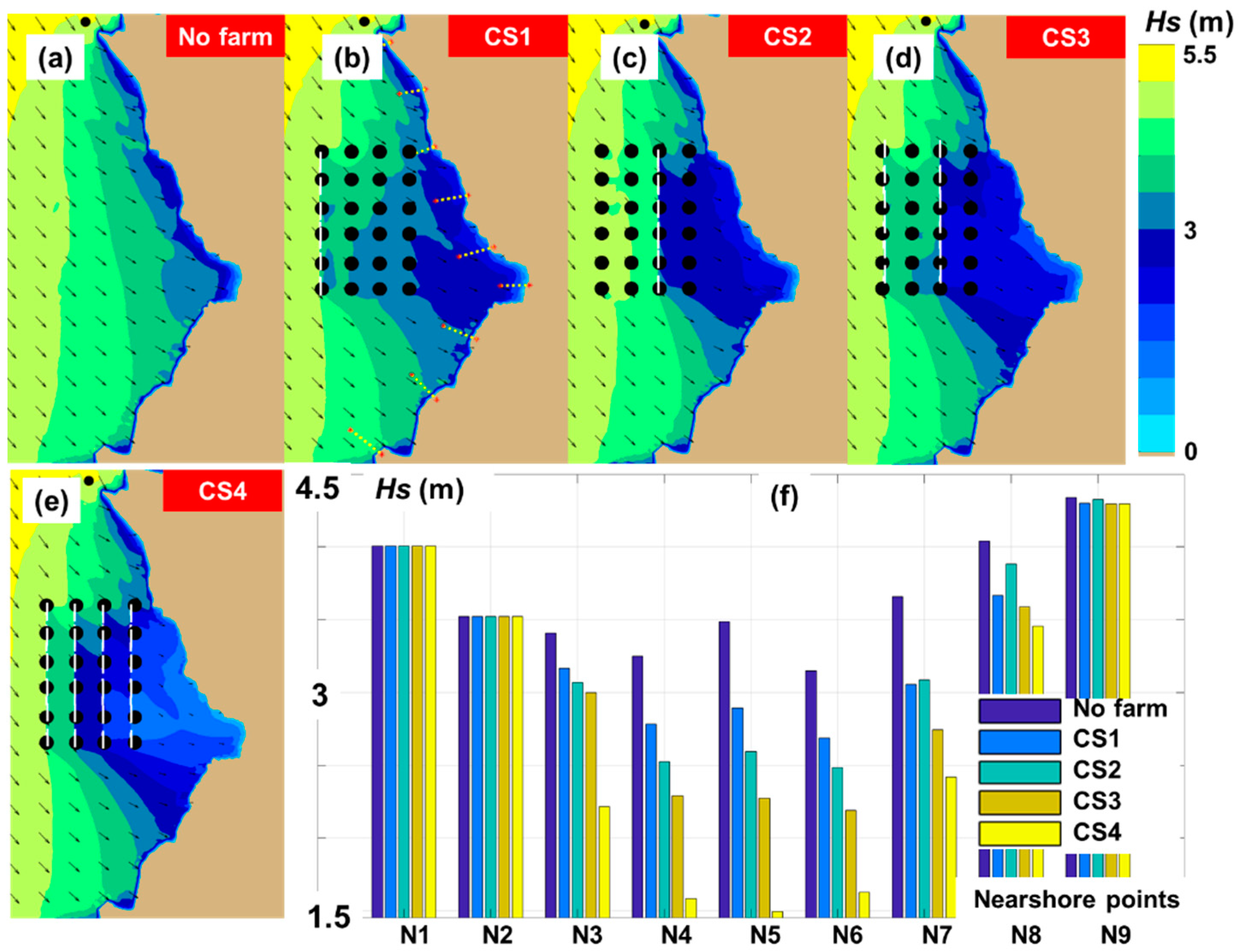
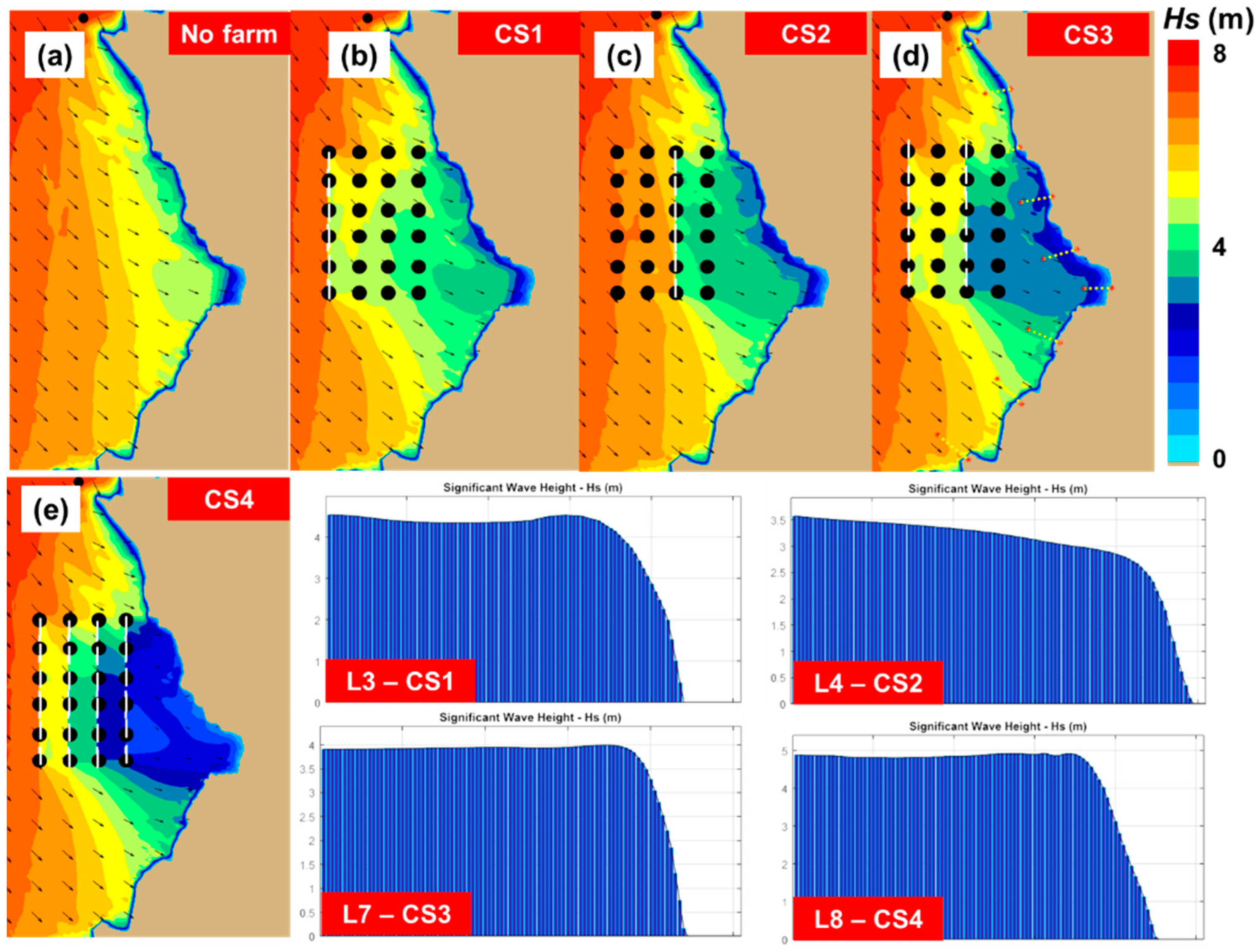
Figure 7 is focused on a high energy summer event, being clearly highlighted the impact of the generic farms in the geographical space, even in the case of the scenario CS1. In this configuration, the shielding effect is more visible in the central part of the target area, especially in front of the Porto Ferro inlet. The variations corresponding to the N-points indicate a similar pattern as the ones presented in
Figure 6f, with the mention that in the case of N7 (
Hs = 3.05 m), a wave farm located offshore (CS1) presents similar results with the ones corresponding to scenario CS2 (
Hs = 3.08 m). The group points N4–N6 indicate lower
Hs values in the case CS4, which drop from 3.5 m (no farm) to a minimum of 1.5 m.
Regarding the variations (in %), these values are included in
Table 4. In general, the erosion processes were accentuated during the storm events, and by looking at these results, we notice that even a single generic farm located offshore (CS1) may reduce the wave heights, this being an expected result from the perspective of the coastal protection. For CS1 the
Hs attenuation starts from 7% and reaches a maximum of 16% near the site N7, located south of Porto Ferro. The highest attenuation corresponds to CS4, around 50%, in the case of the reference points N4–N6.
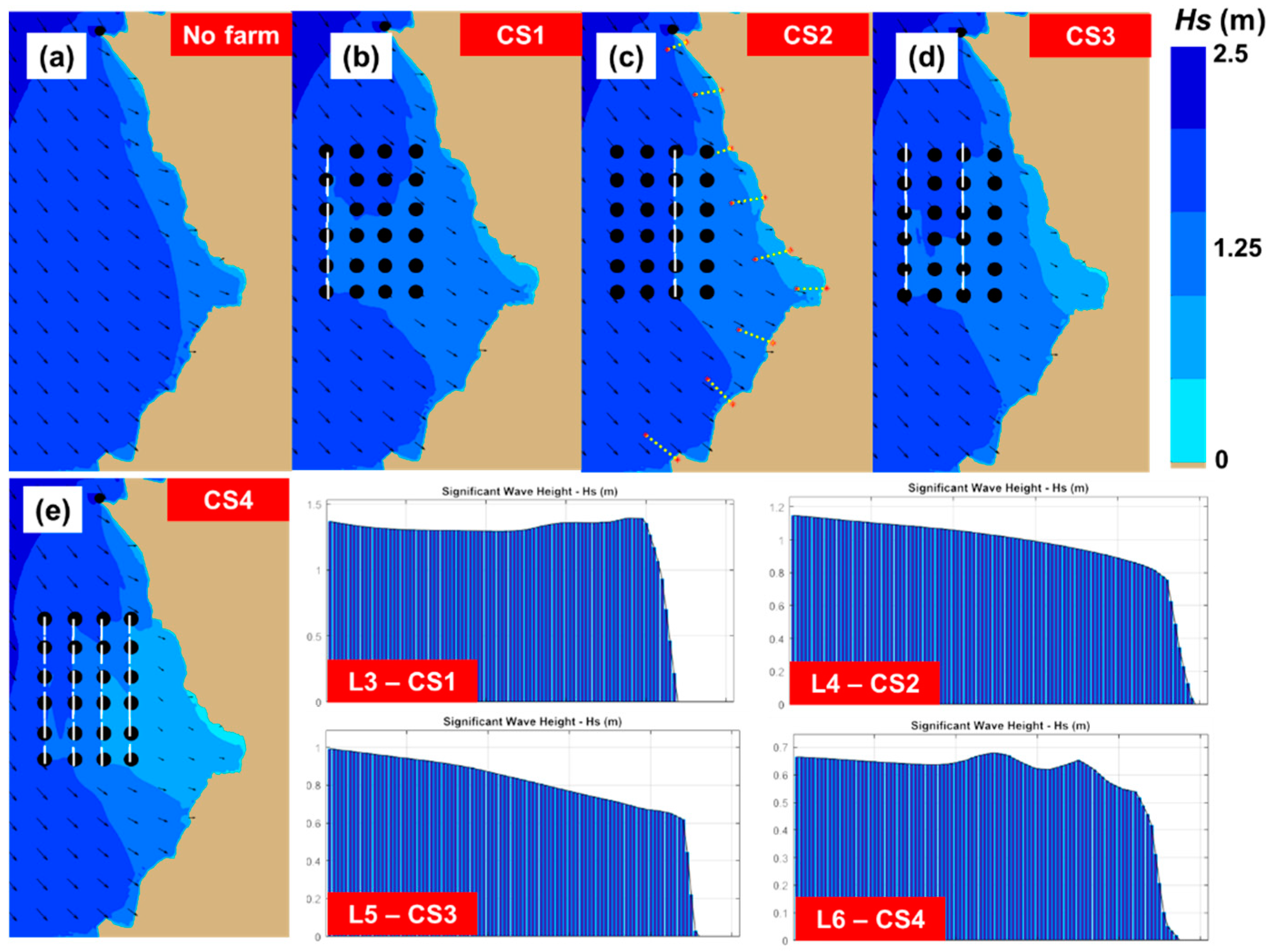
In
Figure 8 and
Table 5, the wave coastal transformation is presented for a typical winter condition. Regardless of the scenario taken into account, there is a visible attenuation of the wave heights, this is the case of CS1 and CS2 when the values can decrease below a threshold of 1.5 m. The changes induced by CS3 and CS4 were more complex, being noticed the occurrence of some multiple wave fields. The highest influence is also between the generic lines. This can be considered a negative effect since the performances of some wave generators were influenced. The wave profiles along several reference lines were presented, each coastal sector indicating particular features. For the lines L3 and L6 there is a constant distribution of the
Hs values until they collapse in the surf zone, being also noticed some bumps for the line L6 that can be associated to the local bathymetry (possible sand bars).
Although the wave characteristics considered were a little higher than those corresponding to the Summer A situation, the differences were relatively close. Nevertheless, for the nearshore points N4–N7 the differences could increase up to 53% compared to only 46% for the summer scenario.
A similar analysis is presented in
Figure 9, considering this time one of the highest wave events that may occur in this region, namely a winter storm. More significant results corresponded to the configuration CS4, which gradually attenuated the wave heights as they passed each generic line, in the context where almost 75% of the waves passed each line. A possible explanation would be that the incoming waves did not have enough space to regenerate, and this disruption was important for the coastal protection. Going closer to the shoreline, we noticed that wave heights were significantly reduced, indicating in general values below 4 m, as the the profile lines L3, L4 and L7 indicate.
The wave variations (
Hs variation in %) are presented in
Table 6. The current profiles along these lines did not change independently of the scenarios considered. However, some modifications were noticed in relationship with current velocity values, in the sense that they decreased from the no farm situation to CS4. The reference points N1–N9 (representing in fact the ends of the reference lines) indicated also these variations, which are presented in
Table 5 and
Table 6. As we go from the scenario CS1 to CS4, various differences were noticed, namely: CS1 to CS2—2% to 9%; CS2 to CS3—2% to 10%; CS3 to CS4—4% to 23%; CS1 to CS3—5% to 18%; and CS1 to CS4—5% to 41%. Taking into account that at this moment there was no operational wind–wave farm, these differences were just for guidance, since it is difficult to estimate what is the standard configuration of a wave farm (ex: how many lines; accepted distance to the shoreline, etc.).
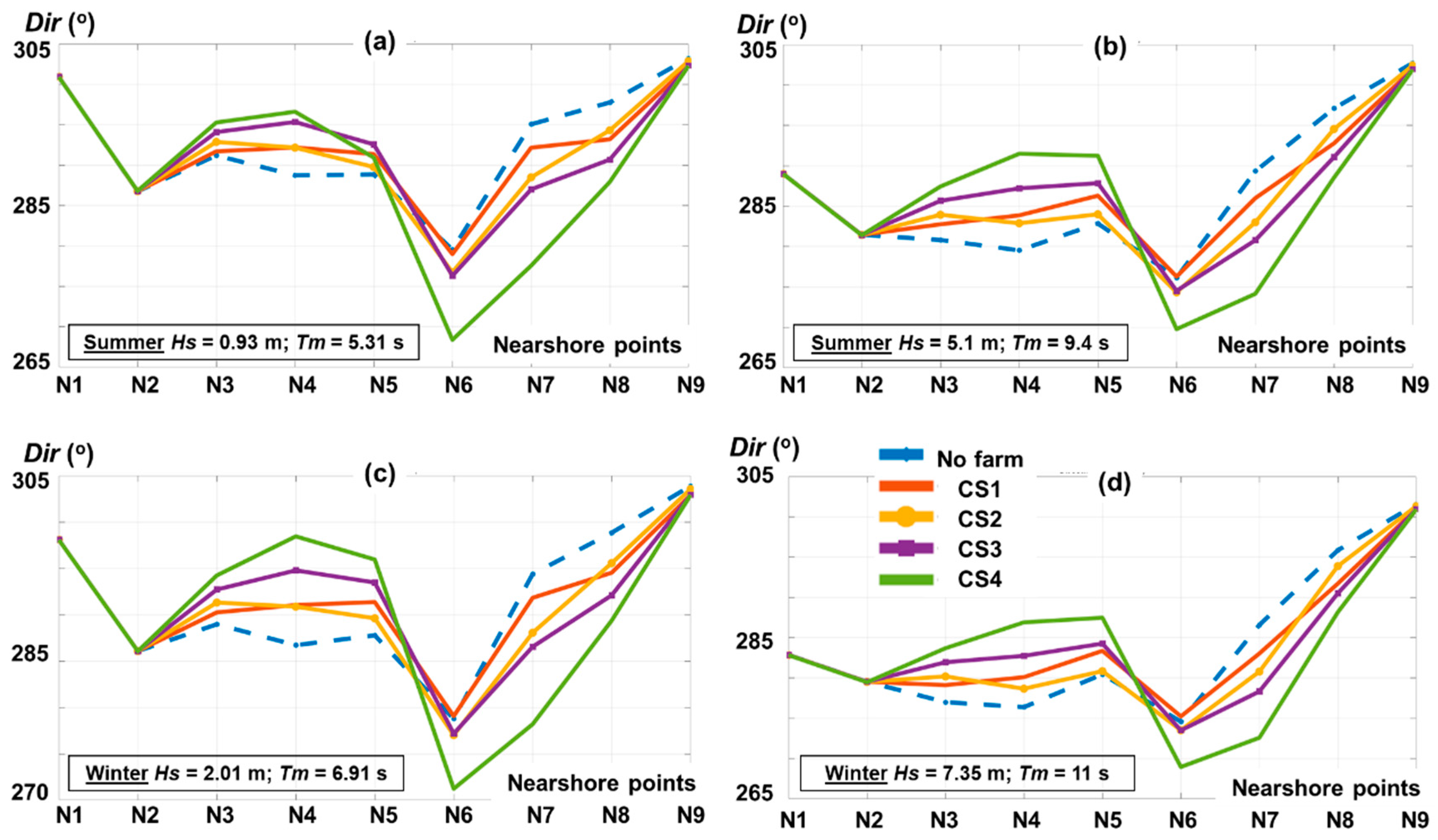
Besides the significant wave heights, some other parameters were important for the coastal processes, this being the case for the wave direction presented in
Figure 10. As expected, the results corresponding to the reference points N1, N2, and N9 did not indicate any variation, while for the group points N3–N5 there was a slight increase in this parameter. For the points N6–N8, the presence of a wave farm may have resulted in a decrease of the wave direction that could influence the erosion processes, especially for the reference point N6 (CS4).
It was noticed that for the summer A scenario (
Figure 10a), the direction could shift from 279.5° to almost 268.4° (N6–CS4) or from 288.7° to 295.3 (N4–CS3). As we went south, the site N8 indicated a gradual variation from 297.8° (no farm) to 294.3
o (CS2); 293.2° (CS1); 290.7° (CS3); or 287.9° (CS4). A similar pattern occurred for the summer B scenario, with the mention that the differences were higher. The direction could vary in the case of site N4 from 279.5° to 283.9° (CS1), reaching a maximum of 291.5° (CS4). For the site N6, the no farm and CS1 scenarios indicated similar values (276.3°). Similar variations were noticed in winter, when during a storm event the generic farm(s) could change the wave pattern from 276.4° to 286.9° (N4–CS4) or from 286.6° to 272.6° (N7–CS4). Since the wave direction is a crucial parameter in the development of the nearshore currents, the fact that the marine energy farm may produce significant changes in terms of wave direction may affect also the longshore current velocity [
36,
44]. That is why, although the waves lost energy in the presence of the marine energy farm, in certain situations due to such changes in wave direction, the longshore current velocity could significantly increase down-wave from a marine energy farm. Such aspects are analyzed next.
3.3. Assessment of the Nearshore Currents
Nearshore currents represent another important element that influence the stability of a beach area, and therefore this section tackles this aspect.
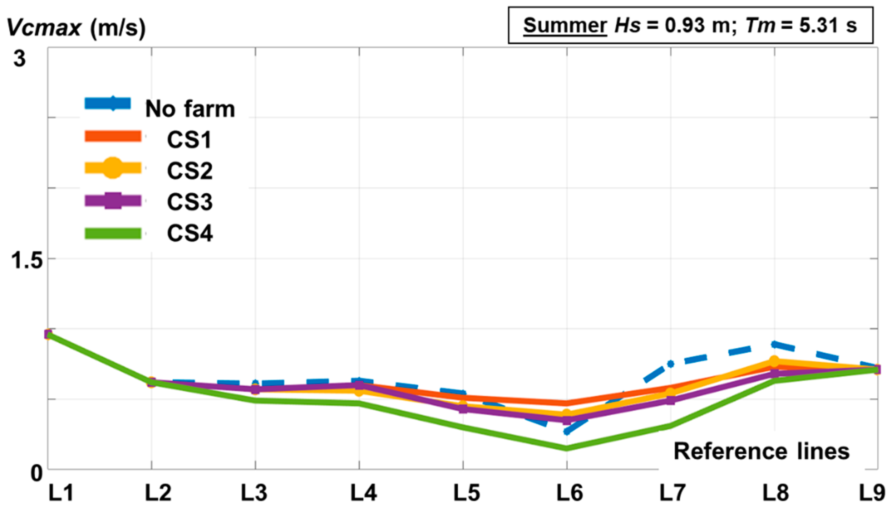
Figure 11 provides a first evaluation for the scenario summer A, where it was be noticed that for the reference lines the currents velocity was reduced, except line L6 (Porto Ferro inlet), where in fact the velocity was amplified for the scenarios CS1–CS3. For example, line L4 indicated a maximum velocity of 0.63 m/s (no farm) that was down to 0.47 m/s (CS4). Line L7 was defined by more significant variations, notably a decrease of the current velocity with almost 23% for CS1 and with a maximum of 41% for CS4. For the line L6, we expected an increase of 74% for CS1 and a decrease of 56% for the CS4, by taking as a reference the current value of 0.27 m/s (corresponding to the no farm situation).
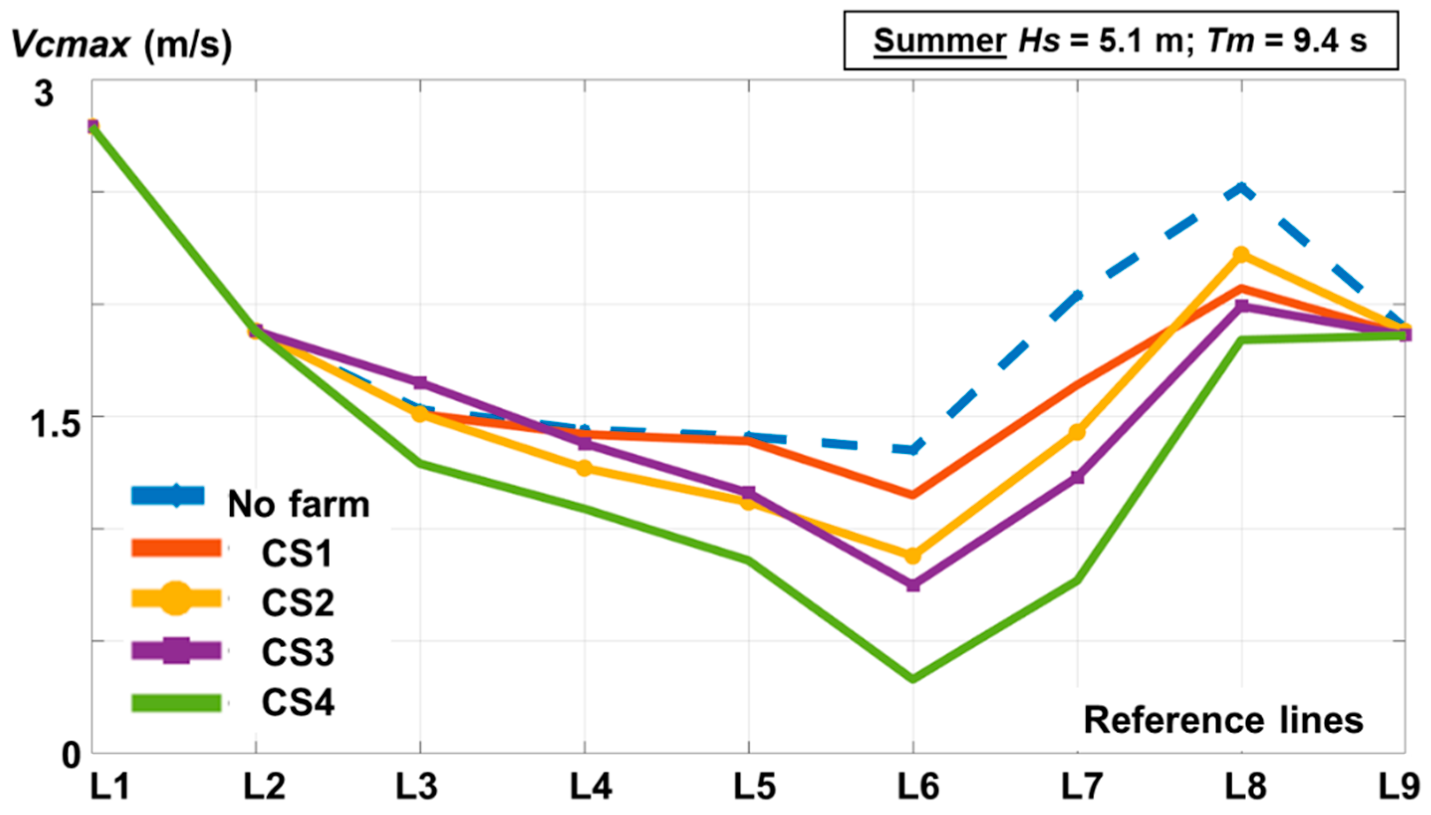
Figure 12 is focused on a high energy summer event, showing in general a decrease of the velocity, except for the lines L3 and L4, where the cases CS1–CS3 indicated no significant impact. Line L6 presented significant variations, the values gradually decreasing from 1.35 m/s to 1.15 m/s (CS1); 0.88 m/s (CS2); 0.75 m/s (CS3); and 0.33 m/s (CS4). Line L7 indicated a maximum decrease, where the currents went from 2.04 m/s to almost 0.77 m/s in the presence of a CS4 configuration.
At this point, it has to be highlighted that, in some cases, the presence of a wave farm could induce various patterns, this being also noticed in Rusu and Onea [
4]. According to these results (Figure 14, point NP1) the current velocity may increase in the presence of a farm defined by moderate absorption and decrease when we consider a high absorption scenario, which is comparable with CS4 used in our work.
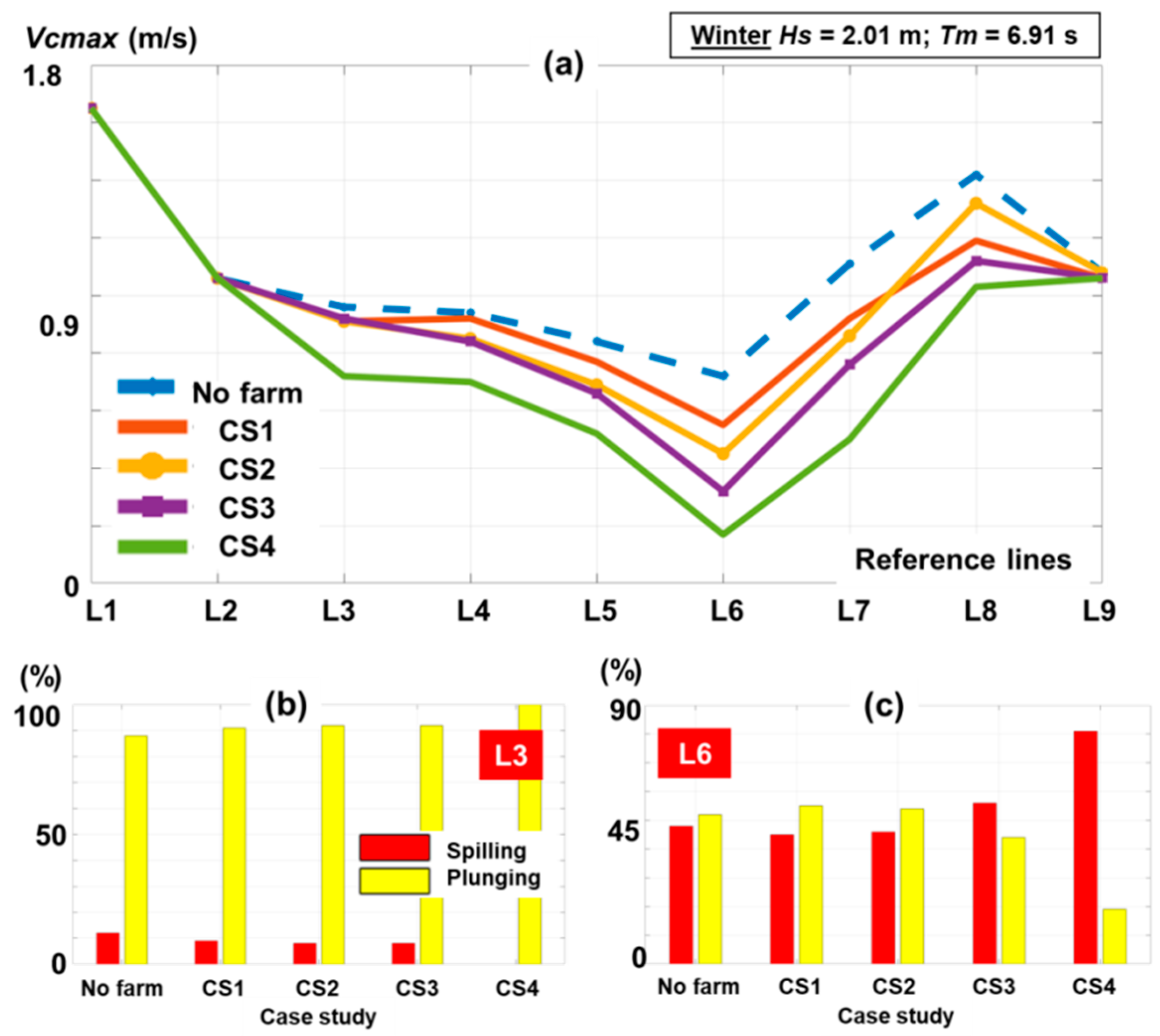
Going to the winter season, a similar pattern was noticed in
Figure 13a, where the velocity oscillated between 0.17 m/s (L6–CS4) and 1.65 m/s (line L1). As the waves entered in the surf area they finally reached their end life and broke under one of the following forms: spilling, plunging, collapsing, or surging. From all these, only the spilling waves interact with the seabed, and therefore would be able to push more sediments into the surf zone [
45]. In
Figure 13b,c, the balance between the breaking waves is presented for two reference lines (L3 and L6), which is divided between spilling and plunging. In the case of line CS4, the plunging waves became dominant (100%) as we went from no farm to CS4, but in the case of line L6, the spilling waves became dominant when a CS3 or CS4 configuration was considered. In a similar way,
Figure 14 presents a high energy winter event that may occur in this region.
Compared to the previous scenarios, for line L5 CS1 and CS2 would have little effect or would accelerate the current velocity, while for the L3 only CS4 would reduce the current velocity from 1.81 m/s to almost 1.62 m/s. In terms of the breaking waves, the reference lines L4 and L7 indicated the plunging waves as being dominant, the impact of the configurations CS3 and CS4 being to accentuate the occurrences of the plunging waves.


